
A New Neighboring Pixels Method for Reducing Aerosol Effects on the NDVI Images


Abstract
:
1. Introduction
2. Methods
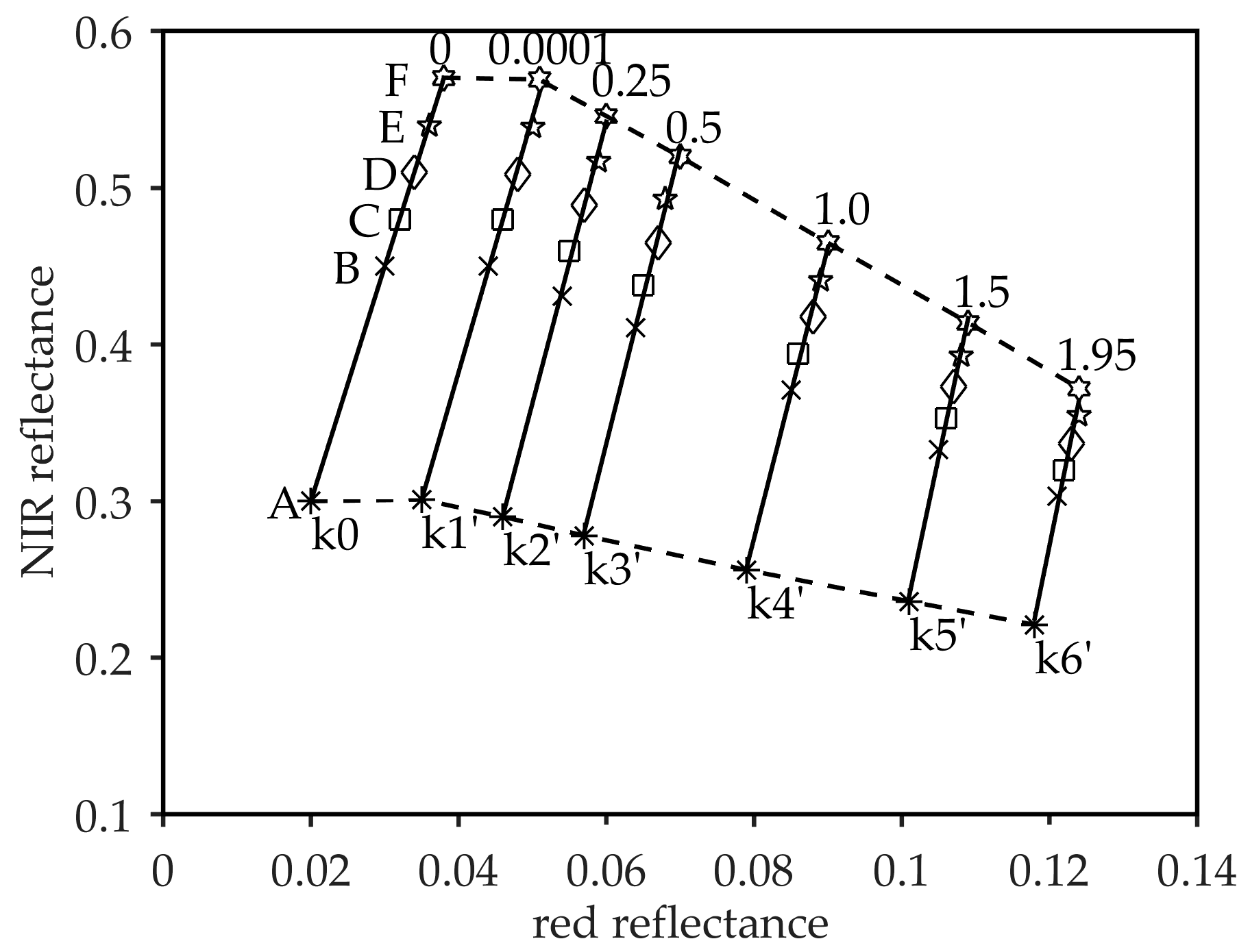
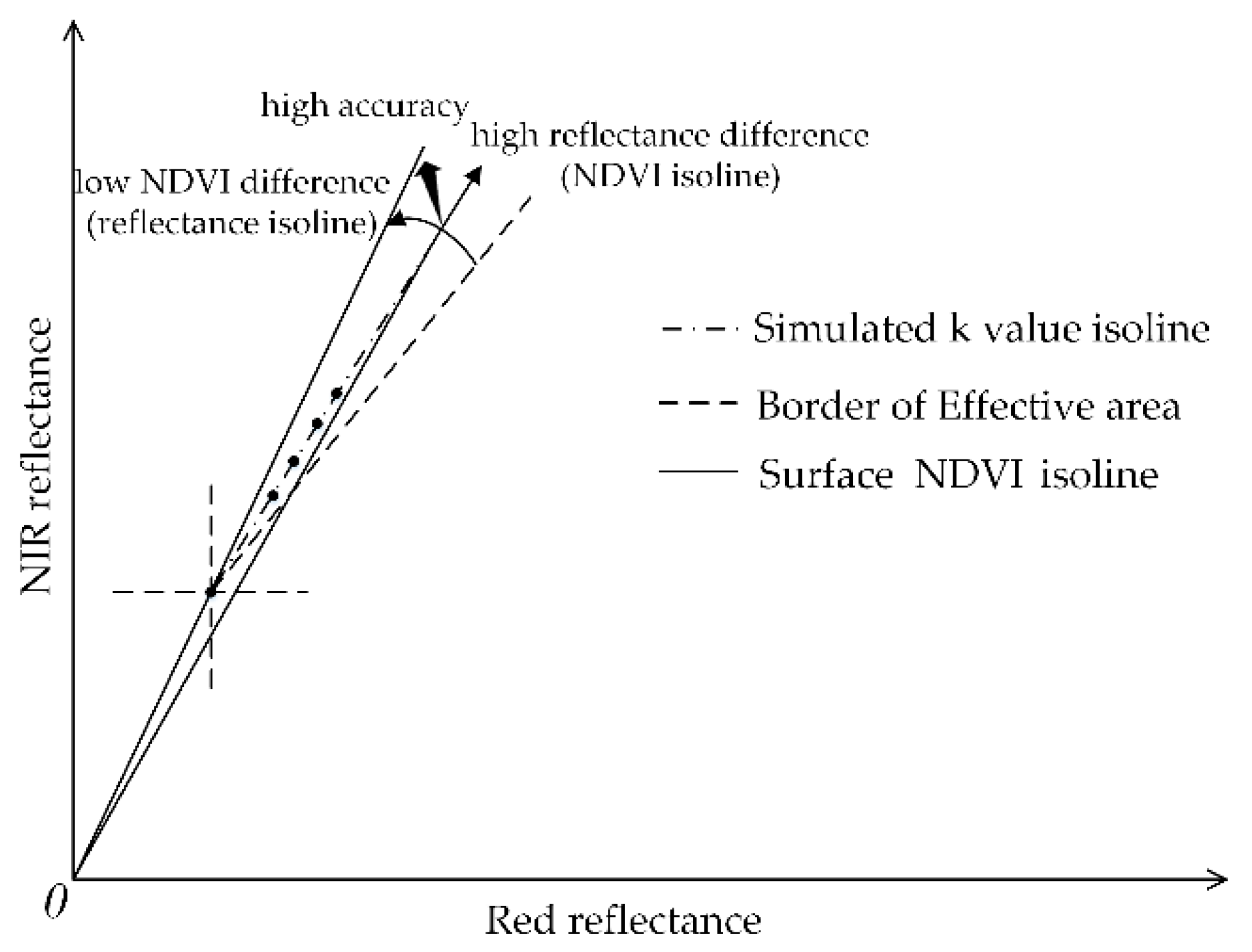
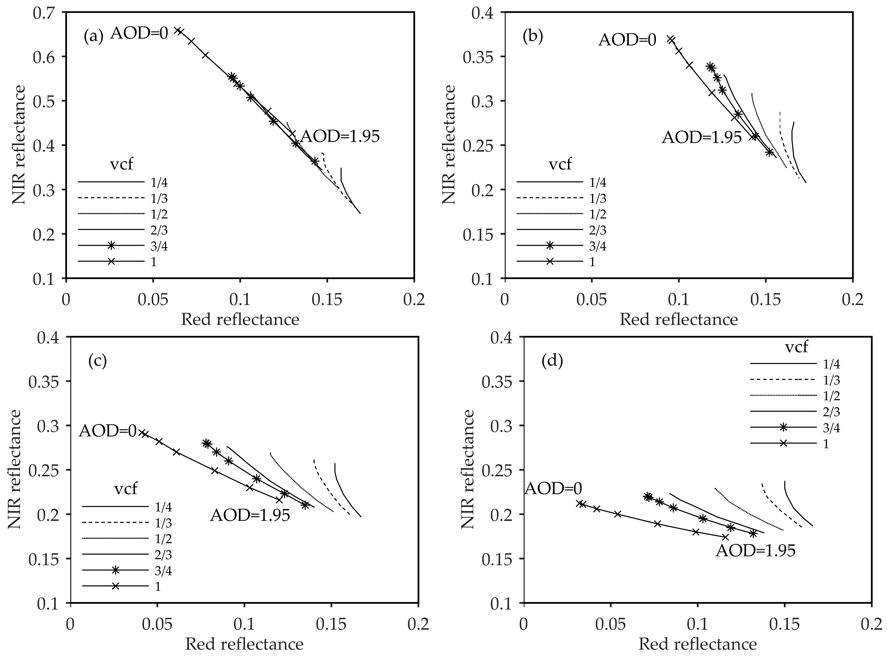
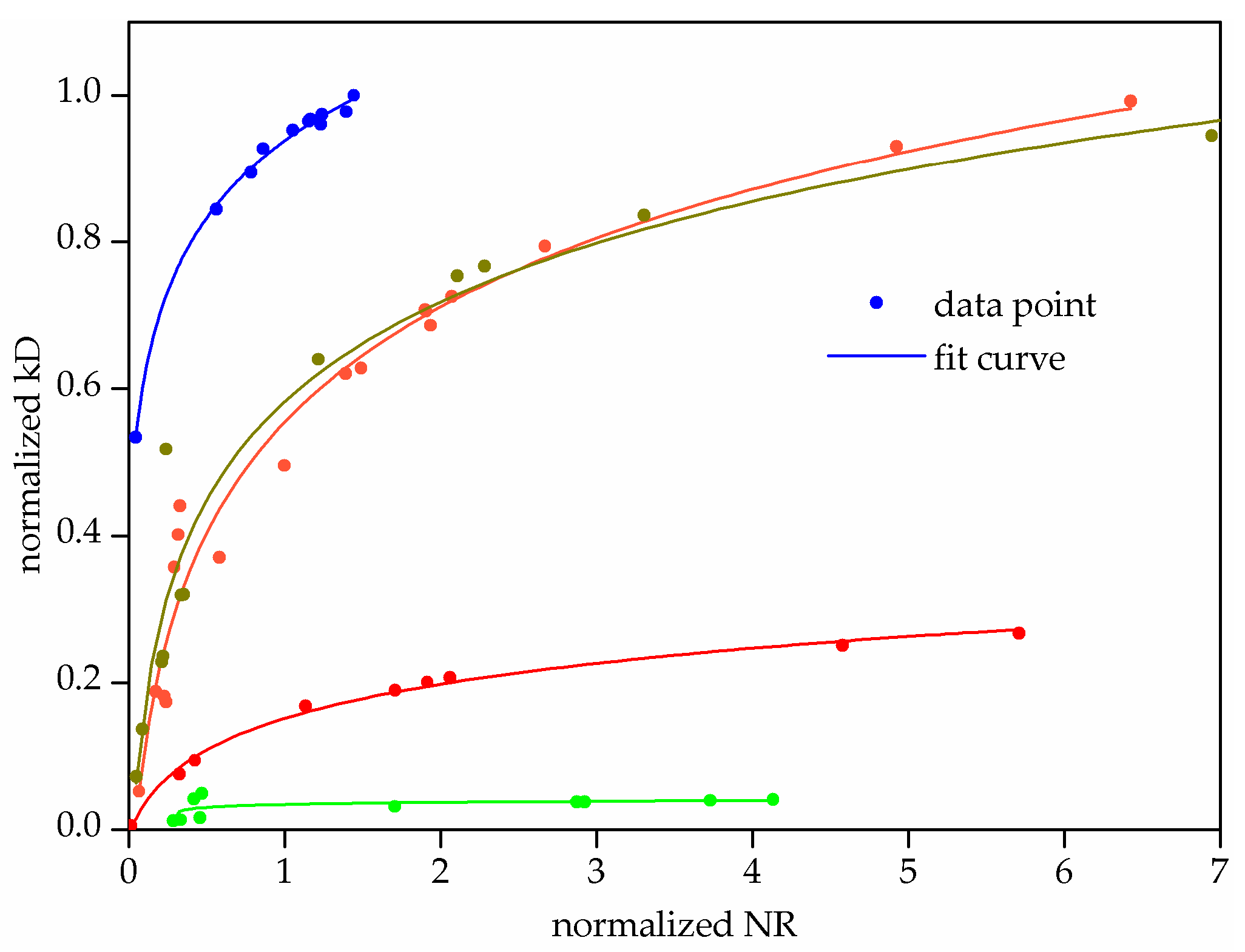
2.1. Vegetation Isolines Simulations Using the 6S Radiative Transfer Code
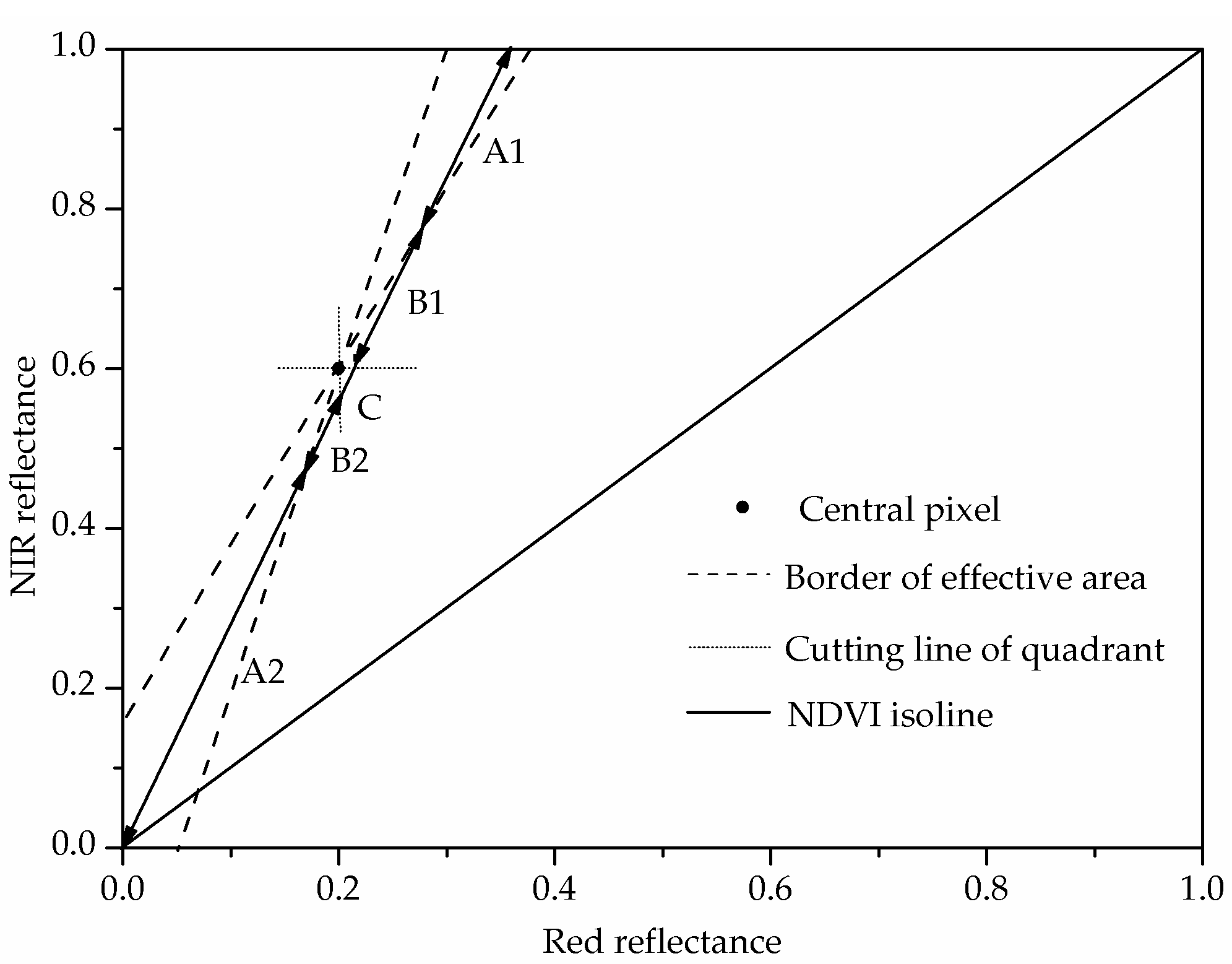
2.2. Derivation of Aerosol Corrected NDVI That Incorporates Neighborhood Information
2.3. Data and Experimental Design
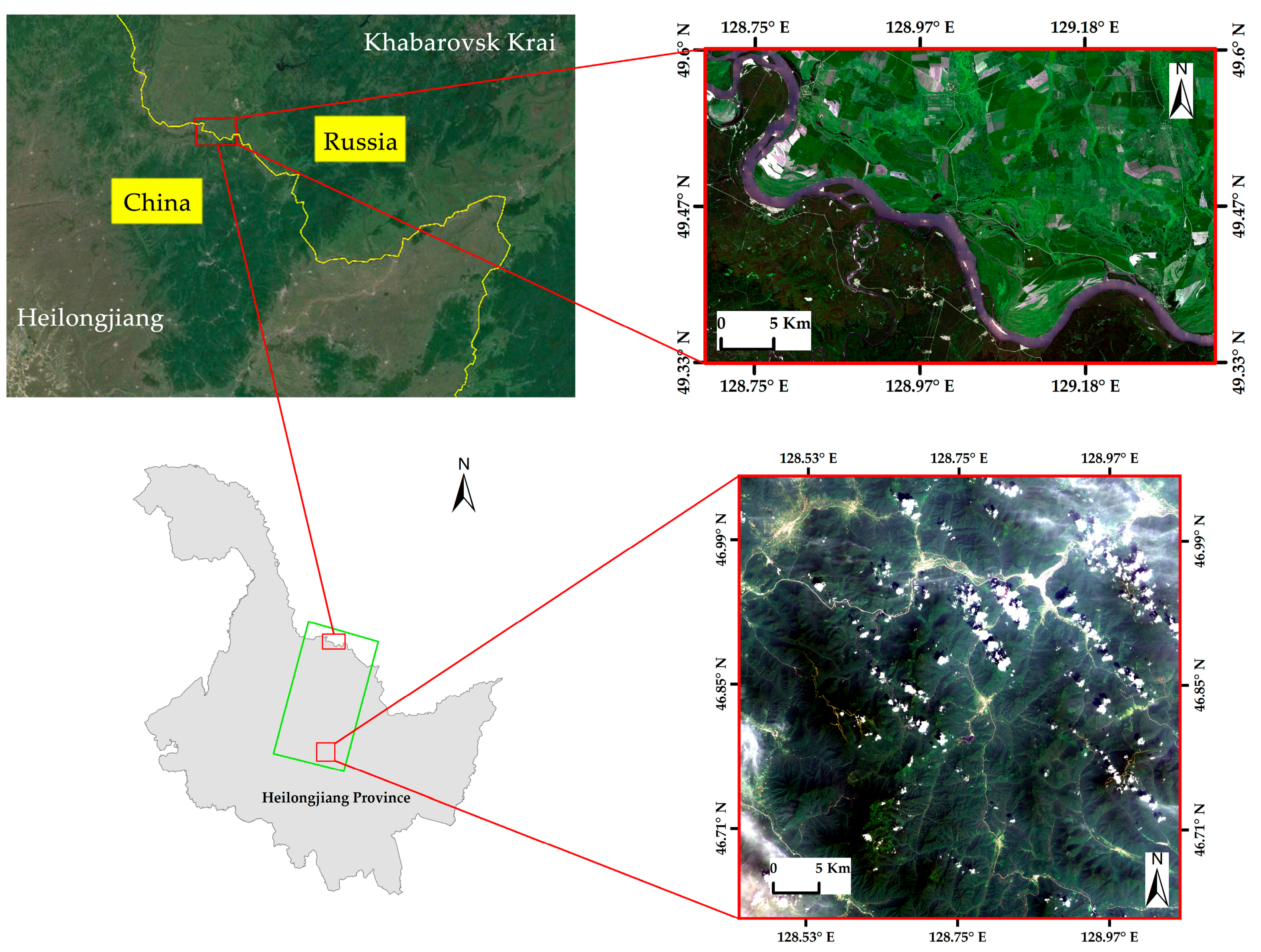
2.3.1. Study Area and Data
2.3.2. Experimental Design
- (1)
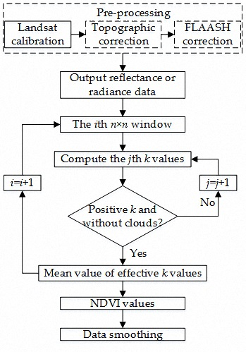
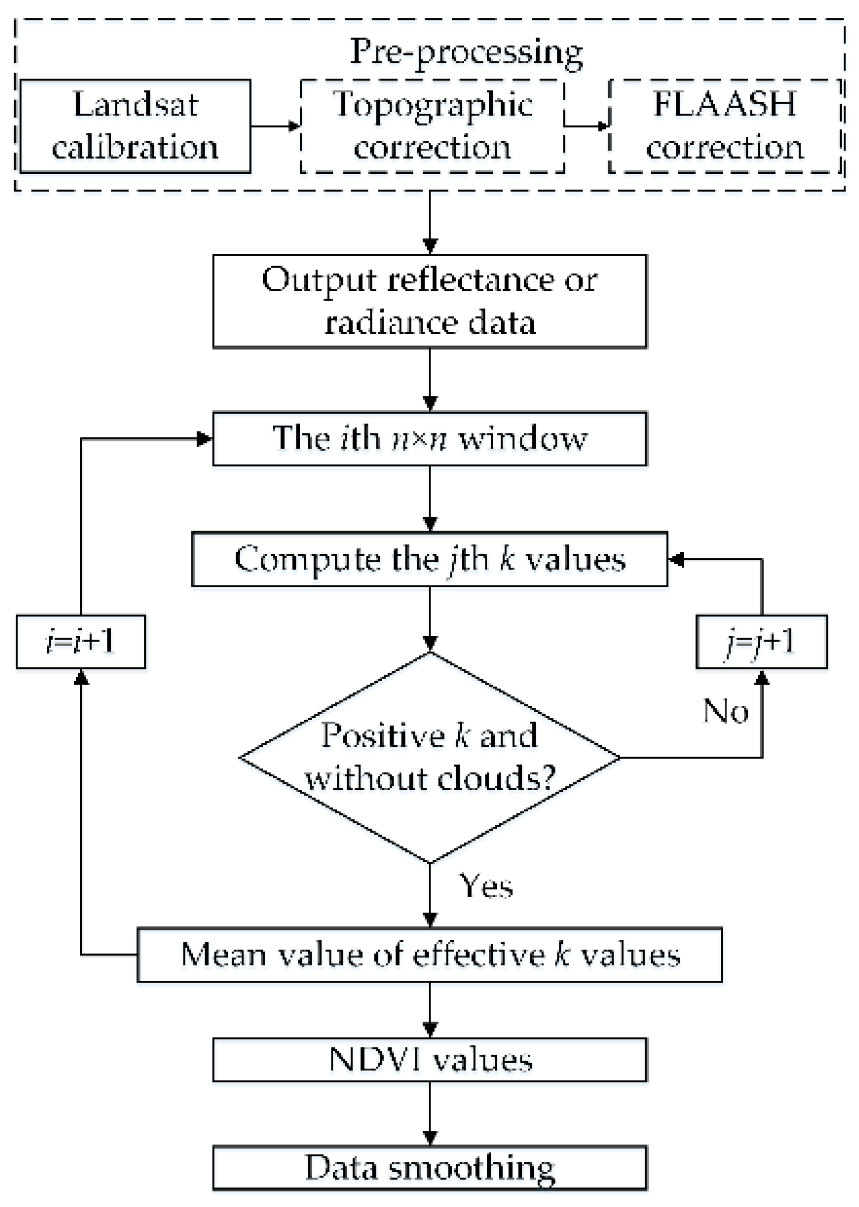
- Pre-processing
- (2)
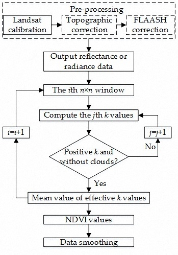
- Algorithm implementation
3. Results
3.1. Optimization of Window Size
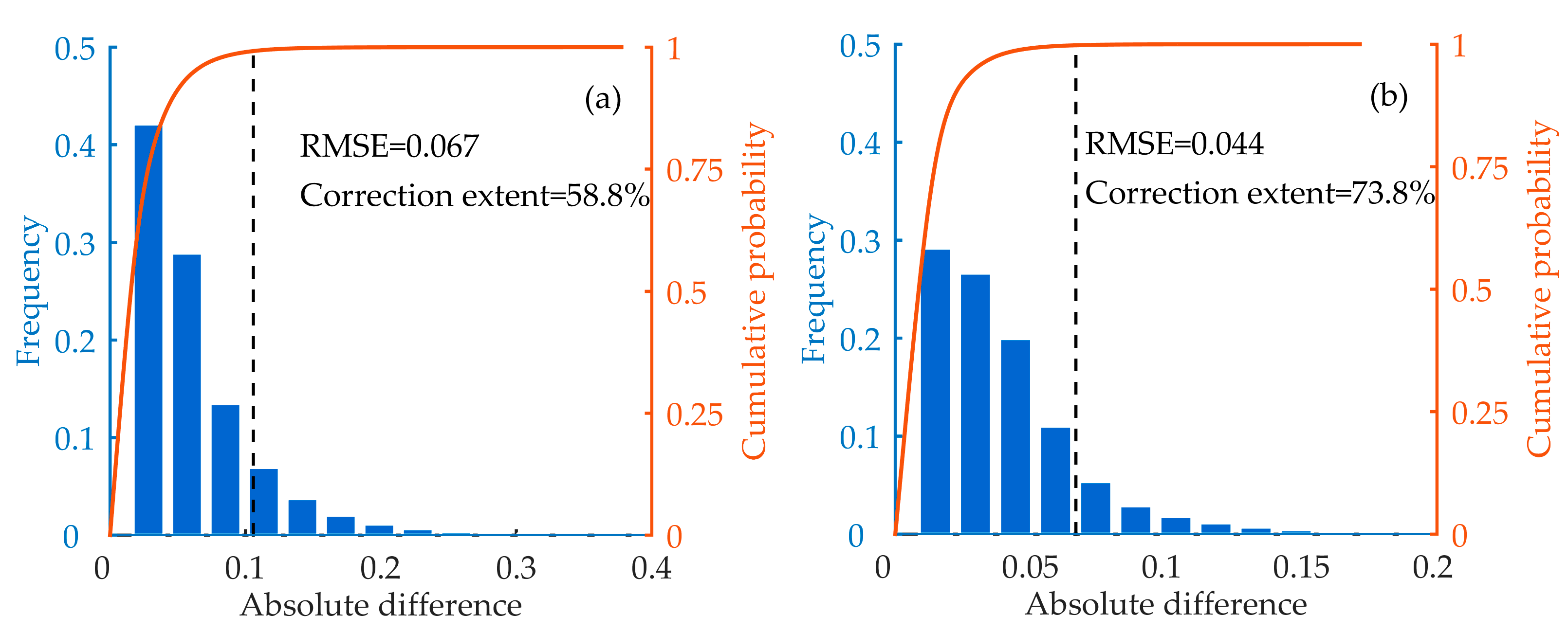
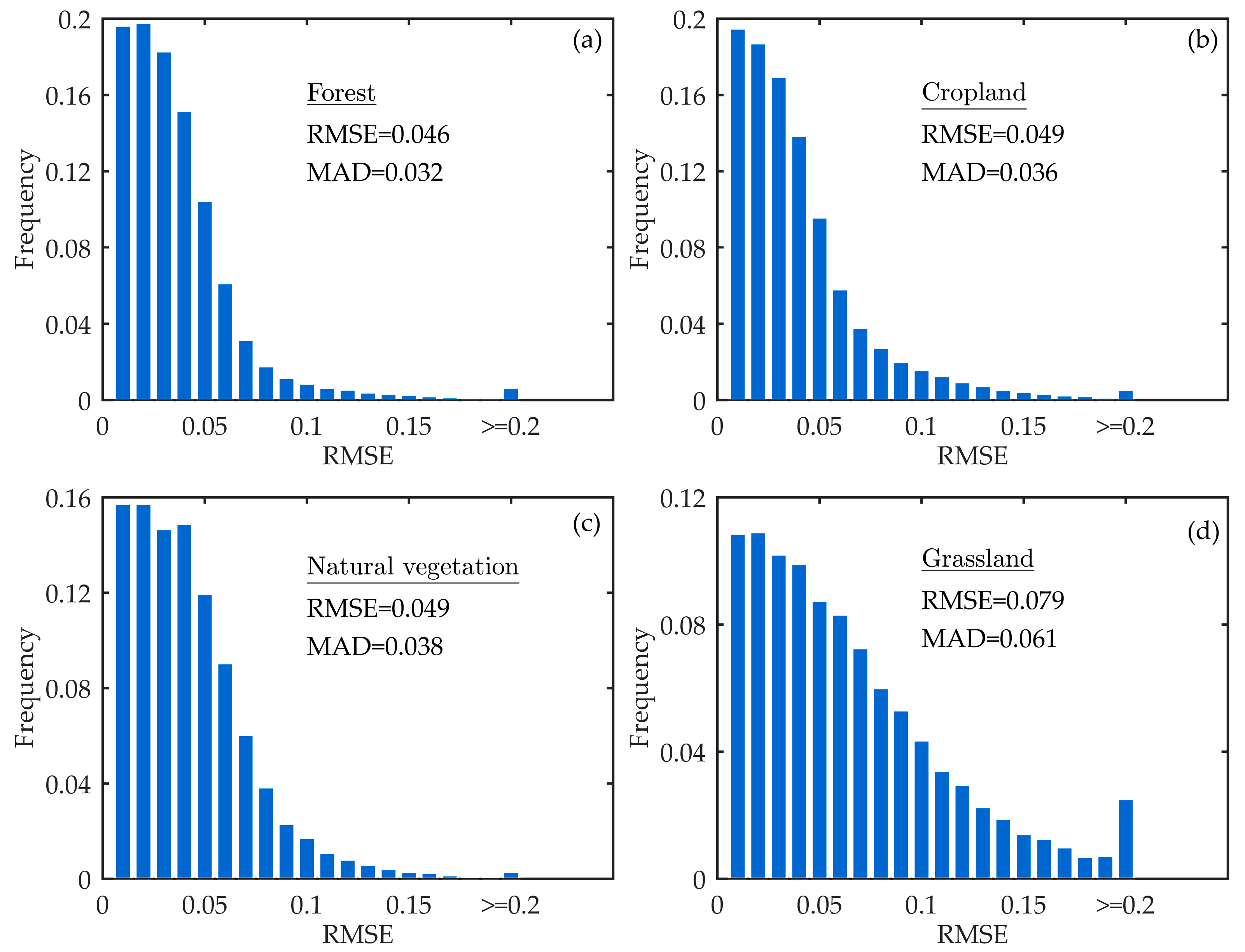
3.2. Accuracy Assessment of Algorithm
3.3. Algorithm Performance under Different Aerosol Loadings
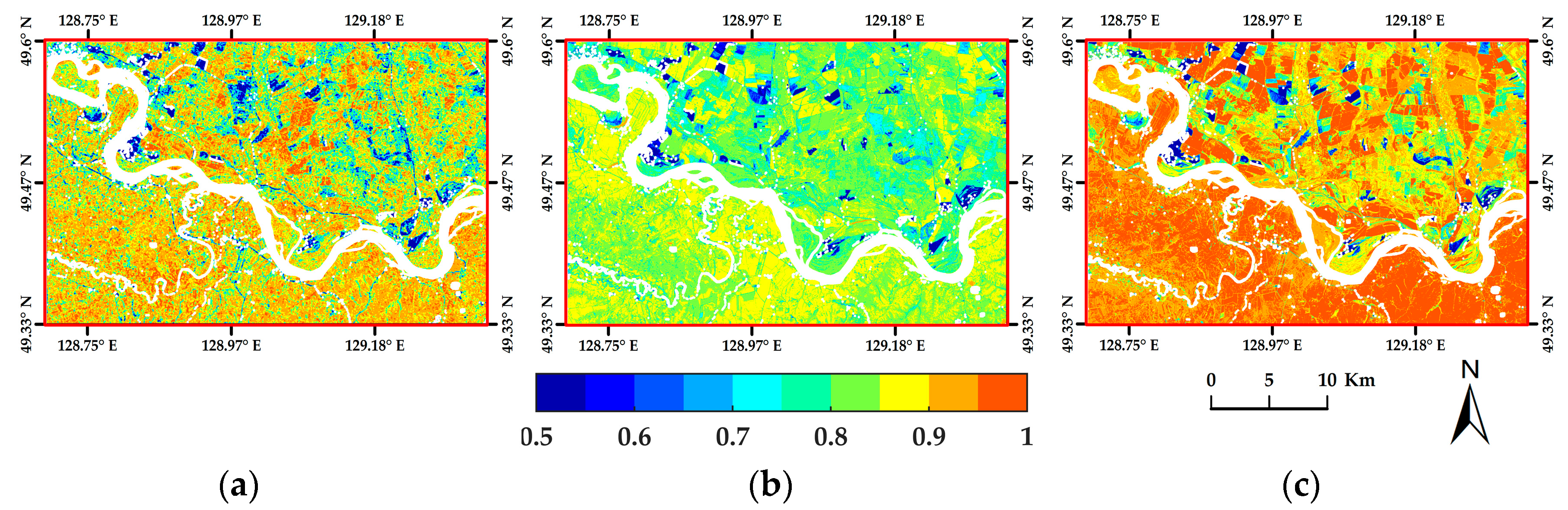
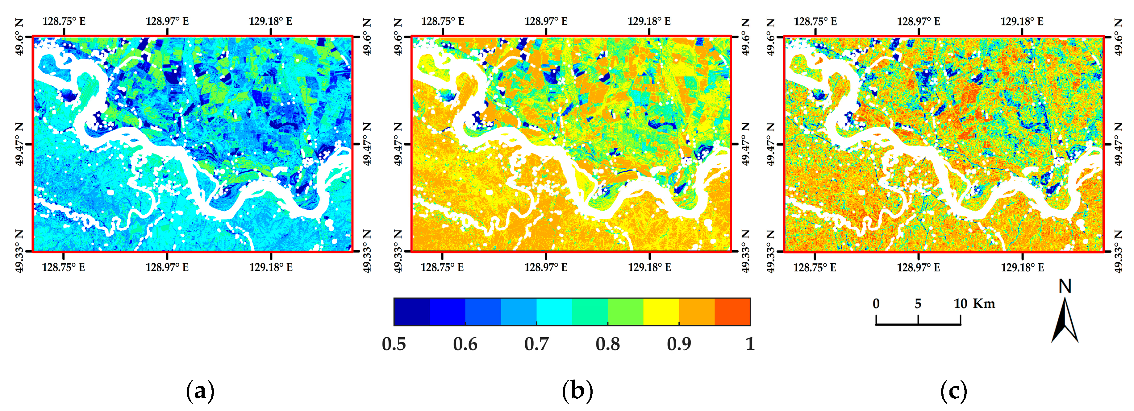
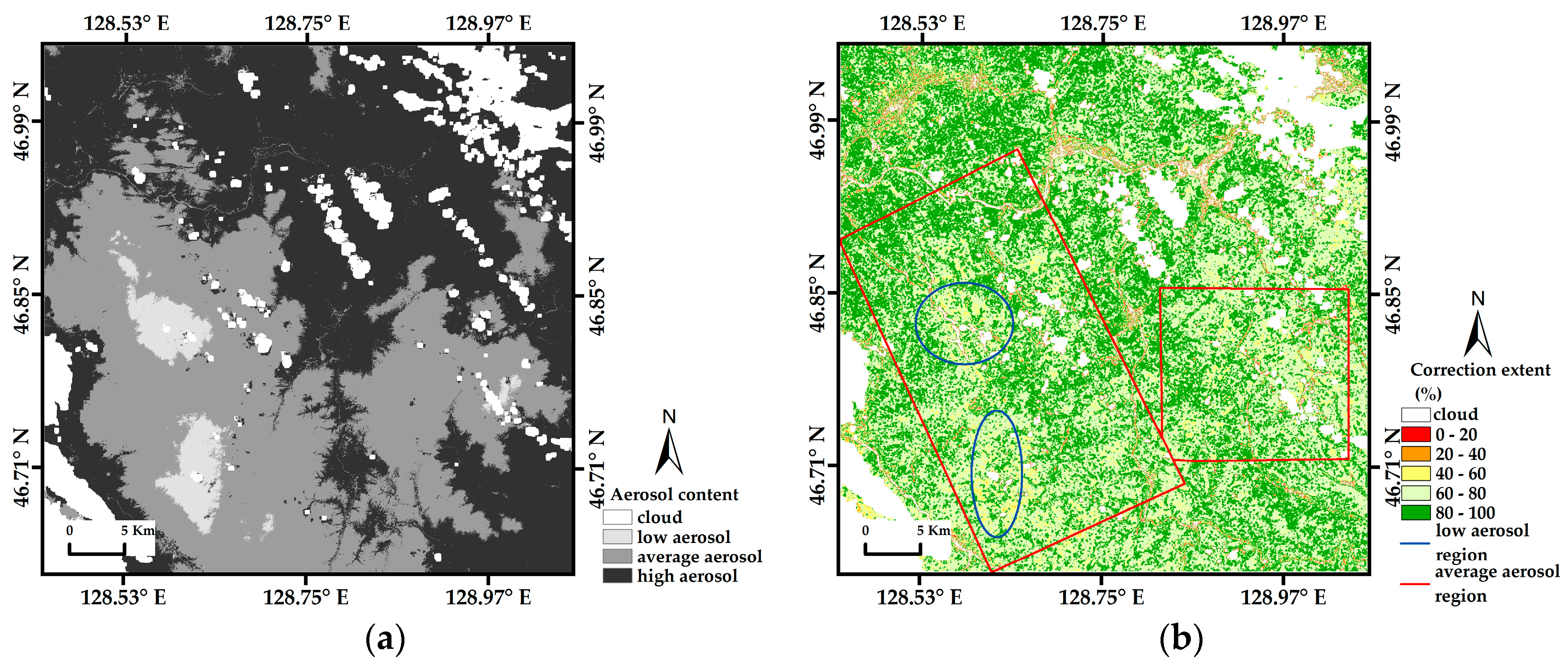
3.4. Application to Atmospheric Correction
4. Discussion
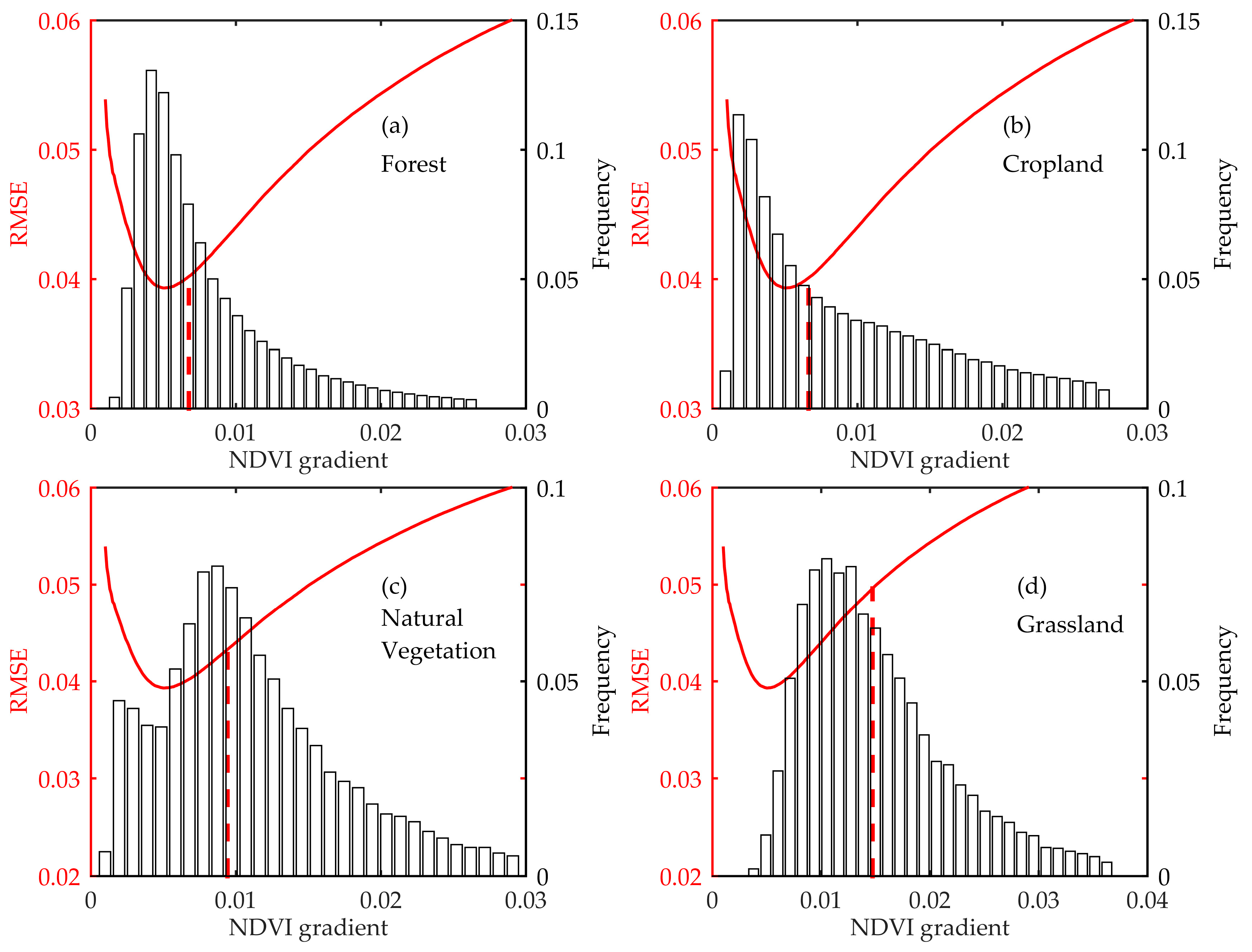
4.1. Factors Influencing Simulation Accuracy
4.2. Possibility of Obtaining an Accurate Aerosol Corrected NDVI
5. Conclusions
Acknowledgments
Author Contributions
Conflicts of Interest
Appendix A

References
- Zhong, B. Improved estimation of aerosol optical depth from Landsat TM/ETM+ imagery over land. In Proceedings of the IEEE International Geoscience and Remote Sensing Symposium, Vancouver, BC, Canada, 24–29 July 2011; pp. 3304–3307.
- Hadjimitsis, D.G. Aerosol optical thickness (AOT) retrieval over land using satellite image-based algorithm. Air Qual. Atmos. Health 2009, 2, 89–97. [Google Scholar] [CrossRef]
- Miura, T.; Huete, A.R.; Yoshioka, H.; Holben, B.N. An error and sensitivity analysis of atmospheric resistant vegetation indices derived from dark target-based atmospheric correction. Remote Sens. Environ. 2001, 78, 284–298. [Google Scholar] [CrossRef]
- Liang, S.; Fallah-Adl, H.; Kalluri, S.; JáJá, J.; Kaufman, Y.J.; Townshend, J.R.G. An operational atmospheric correction algorithm for Landsat Thematic Mapper imagery over the land. J. Geophys. Res. 1997, 102. [Google Scholar] [CrossRef]
- Huete, A.; Justice, C.; van Leeuwen, W. Modis Vegetation Index (MOD13). Algorithm Theor. Basis Doc. 1999, 3, 213. [Google Scholar]
- Tanré, D.; Kaufman, Y.; Herman, M.; Mattoo, S. Remote sensing of aerosol properties over oceans using the MODIS/EOS spectral radiances. J. Geophys. Res. 1997, 102, 16971–16988. [Google Scholar] [CrossRef]
- Kaufman, Y.; Tanré, D.; Remer, L.A.; Vermote, E.; Chu, A.; Holben, B. Operational remote sensing of tropospheric aerosol over land from EOS moderate resolution imaging spectroradiometer. J. Geophys. Res. 1997, 102, 17051–17067. [Google Scholar] [CrossRef]
- Hsu, N.C.; Tsay, S.C.; King, M.D.; Herman, J.R. Aerosol properties over bright-reflecting source regions. IEEE Trans. Geosci. Remote Sens. 2004, 42, 557–569. [Google Scholar] [CrossRef]
- Hsu, N.C.; Tsay, S.C.; King, M.D.; Herman, J.R. Deep blue retrievals of Asian aerosol properties during ACE-Asia. IEEE Trans. Geosci. Remote Sens. 2006, 44, 3180–3195. [Google Scholar] [CrossRef]
- Hsu, N.; Jeong, M.J.; Bettenhausen, C.; Sayer, A.; Hansell, R.; Seftor, C.; Huang, J.; Tsay, S.C. Enhanced deep blue aerosol retrieval algorithm: The second generation. J. Geophys. Res. 2013, 118, 9296–9315. [Google Scholar] [CrossRef]
- Tanré, D.; Deschamps, P.; Devaux, C.; Herman, M. Estimation of Saharan aerosol optical thickness from blurring effects in Thematic Mapper data. J. Geophys. Res. 1988, 93, 15955–15964. [Google Scholar] [CrossRef]
- Kaufman, Y.J.; Wald, A.E.; Remer, L.; Gao, B.C.; Li, R.-R.; Flynn, L. The MODIS 2.1-μm channel-correlation with visible reflectance for use in remote sensing of aerosol. IEEE Trans. Geosci. Remote Sens. 1997, 35, 1286–1298. [Google Scholar] [CrossRef]
- Levy, R.C.; Remer, L.A.; Mattoo, S.; Vermote, E.F.; Kaufman, Y.J. Second-generation operational algorithm: Retrieval of aerosol properties over land from inversion of Moderate Resolution Imaging Spectroradiometer spectral reflectance. J. Geophys. Res. 2007, 112. [Google Scholar] [CrossRef]
- Levy, R.; Mattoo, S.; Munchak, L.; Remer, L.; Sayer, A.; Hsu, N. The collection 6 MODIS aerosol products over land and ocean. Atmos. Meas. Tech. 2013, 6, 2989–3034. [Google Scholar] [CrossRef]
- Ouaidrari, H.; Vermote, E.F. Operational atmospheric correction of Landsat TM data. Remote Sens. Environ. 1999, 70, 4–15. [Google Scholar] [CrossRef]
- Zhao, W.H.; Gong, H.; Zhao, W.J.; Li, X.J. The distribution of aerosol optical depth retrieved by TM imagery over Beijing urban area, China. In Proceedings of the IEEE International Geoscience and Remote Sensing Symposium, Vancouver, BC, Canada, 24–29 July 2011; pp. 2185–2188.
- Bilal, M.; Nichol, J.E.; Bleiweiss, M.P.; Dubois, D. A simplified high resolution MODIS Aerosol Retrieval Algorithm (SARA) for use over mixed surfaces. Remote Sens. Environ. 2013, 136, 135–145. [Google Scholar] [CrossRef]
- Bilal, M.; Nichol, J.E.; Chan, P.W. Validation and accuracy assessment of a Simplified Aerosol Retrieval Algorithm (SARA) over Beijing under low and high aerosol loadings and dust storms. Remote Sens. Environ. 2014, 153, 50–60. [Google Scholar] [CrossRef]
- Bilal, M.; Nichol, J.E. Evaluation of MODIS aerosol retrieval algorithms over the Beijing-Tianjin-Hebei region during low to very high pollution events. J. Geophys. Res. 2015, 120, 7941–7957. [Google Scholar] [CrossRef]
- Kaufman, Y.J.; Tanre, D. Atmospherically resistant vegetation index (ARVI) for EOS-MODIS. IEEE Trans. Geosci. Remote Sens. 1992, 30, 261–270. [Google Scholar] [CrossRef]
- Liu, H.Q.; Huete, A. A feedback based modification of the NDVI to minimize canopy background and atmospheric noise. IEEE Trans. Geosci. Remote Sens. 1995, 33, 457–465. [Google Scholar]
- Huete, A.; Didan, K.; Miura, T.; Rodriguez, E.P.; Gao, X.; Ferreira, L.G. Overview of the radiometric and biophysical performance of the MODIS vegetation indices. Remote Sens. Environ. 2002, 83, 195–213. [Google Scholar] [CrossRef]
- Jiang, Z.; Huete, A.R.; Didan, K.; Miura, T. Development of a two-band enhanced vegetation index without a blue band. Remote Sens. Environ. 2008, 112, 3833–3845. [Google Scholar] [CrossRef]
- Karnieli, A.; Kaufman, Y.J.; Remer, L.; Wald, A. AFRI—Aerosol free vegetation index. Remote Sens. Environ. 2001, 77, 10–21. [Google Scholar] [CrossRef]
- He, J.; Zha, Y.; Zhang, J.; Gao, J. Aerosol indices derived from MODIS data for indicating aerosol-induced air pollution. Remote Sens. 2014, 6, 1587–1604. [Google Scholar] [CrossRef]
- Gillingham, S.; Flood, N.; Gill, T.; Mitchell, R. Limitations of the dense dark vegetation method for aerosol retrieval under Australian conditions. Remote Sens. Lett. 2012, 3, 67–76. [Google Scholar] [CrossRef]
- Shi, Y.; Zhang, J.; Reid, J.; Hyer, E.; Hsu, N. Critical evaluation of the MODIS deep blue aerosol optical depth product for data assimilation over North Africa. Atmos. Meas. Tech. 2013, 6, 949–969. [Google Scholar] [CrossRef]
- Kaufman, Y.J. Satellite sensing of aerosol absorption. J. Geophys. Res. 1987, 92, 4307–4317. [Google Scholar] [CrossRef]
- Huete, A.; Jackson, R. Suitability of spectral indices for evaluating vegetation characteristics on arid rangelands. Remote Sens. Environ. 1987, 23. [Google Scholar] [CrossRef]
- Huete, A.; Jackson, R.; Post, D. Spectral response of a plant canopy with different soil backgrounds. Remote Sens. Environ. 1985, 17, 37–53. [Google Scholar] [CrossRef]
- Muldashev, T.; Lyapustin, A.; Sultangazin, U. Spherical harmonics method in the problem of radiative transfer in the atmosphere-surface system. J. Quant. Spectrosc. Radiat. Transf. 1999, 61, 393–404. [Google Scholar] [CrossRef]
- Kotchenova, S.Y.; Vermote, E.F.; Matarrese, R.; Klemm, F.J., Jr. Validation of a vector version of the 6S radiative transfer code for atmospheric correction of satellite data. Part I: Path radiance. Appl. Opt. 2006, 45, 6762–6774. [Google Scholar] [PubMed]
- Vermote, E.F.; Saleous, M.N. Operational atmospheric correction of MODIS visible to middle infrared land surface data in the case of an infinite lambertian target. In Earth Science Satellite Remote Sensing; Springer: Berlin, Germany, 2006; pp. 123–153. [Google Scholar]
- Bassani, C.; Manzo, C.; Braga, F.; Bresciani, M.; Giardino, C.; Alberotanza, L. The impact of the microphysical properties of aerosol on the atmospheric correction of hyperspectral data in coastal waters. Atmos. Meas. Tech. 2015, 8, 1593–1604. [Google Scholar] [CrossRef]
- Ma, Y.; Li, Z.Q.; Li, H.; Hou, W.Z.; Zhang, Y.H.; Li, D.H.; Zhang, Y.; Li, K.T.; Chen, C. Influence of aerosol model in the atmospheric correction of salellite images-a case study over Tianjin region. Remote Sens. Technol. Appl. 2014, 29, 410–418. [Google Scholar]
- Zhang, Y.; Li, Z.; Hou, W.; Li, D.; Zhang, Y.; Ma, Y. Assessment of aerosol models to AOD retrieval from HJ1 satellites. In Proceedings of the IOP Conference Series: Earth and Environmental Science, 35th International Symposium on Remote Sensing of Environment, Beijing, China, 21–26 April 2013.
- Vermote, E.; Tanré, D.; Deuzé, J.; Herman, M.; Morcrette, J.; Kotchenova, S. Second Simulation of A Satellite Signal in the Solar Spectrum-Vector (6SV). 6S User Guide Vers. 2006, 3, 1–55. [Google Scholar]
- Eck, T.; Holben, B.; Reid, J.; Dubovik, O.; Smirnov, A.; O’neill, N.; Slutsker, I.; Kinne, S. Wavelength dependence of the optical depth of biomass burning, urban, and desert dust aerosols. J. Geophys. Res. 1999, 104, 31333–31349. [Google Scholar] [CrossRef]
- Bowker, D.E.; Davis, R.E.; Myrick, D.L.; Stacy, K.; Jones, W.T. Spectral Reflectances of Natural Targets for Use in Remote Sensing Studies; Technical Report for NASA Langley Research Center: Hampton, VA, USA, 1985. [Google Scholar]
- Kaufman, Y.; Tanré, D.; Holben, B.; Markham, B.; Gitelson, A.A. Atmospheric effects on the NDVI-strategies for its removal. In Proceedings of the IEEE International Geoscience and Remote Sensing Symposium, Houston, TX, USA, 26–29 May 1992; pp. 1238–1241.
- Liu, G.R.; Liang, C.K.; Kuo, T.H.; Huang, S.J. Comparison of the NDVI, ARVI and AFRI vegetation index, along with their relations with the AOD using SPOT 4 vegetation data. Terrestr. Atmos. Ocean. Sci. 2004, 15, 15–31. [Google Scholar]
- Tanré, D.; Holben, B.N.; Kaufman, Y.J. Atmospheric correction against algorithm for NOAA-AVHRR products: Theory and application. IEEE Trans. Geosci. Remote Sens. 1992, 30, 231–248. [Google Scholar] [CrossRef]
- Skidmore, A. Environmental Modelling with GIS and Remote Sensing; Taylor and Francis: London, UK, 2002. [Google Scholar]
- Goward, S.N.; Markham, B.; Dye, D.G.; Dulaney, W.; Yang, J. Normalized difference vegetation index measurements from the Advanced Very High Resolution Radiometer. Remote Sens. Environ. 1991, 35, 257–277. [Google Scholar] [CrossRef]
- Richter, R.; Kellenberger, T.; Kaufmann, H. Comparison of topographic correction methods. Remote Sens. 2009, 1, 184–196. [Google Scholar] [CrossRef]
- Fung, T. An assessment of TM imagery for land-cover change detection. IEEE Trans. Geosci. Remote Sens. 1990, 28, 681–684. [Google Scholar] [CrossRef]
- Nehrir, A.R.; Repasky, K.S.; Reagan, J.A.; Carlsten, J.L. Optical characterization of continental and biomass-burning aerosols over Bozeman, Montana: A case study of the aerosol direct effect. J. Geophys. Res. 2011, 116. [Google Scholar] [CrossRef]
- Qie, L.; Li, Z.; Sun, X.; Sun, B.; Li, D.; Liu, Z.; Huang, W.; Wang, H.; Chen, X.; Hou, W. Improving remote sensing of aerosol optical depth over land by polarimetric measurements at 1640 nm: Airborne test in north china. Remote Sens. 2015, 7, 6240–6256. [Google Scholar] [CrossRef]
- Chen, J.; Zhu, X.; Vogelmann, J.E.; Gao, F.; Jin, S. A simple and effective method for filling gaps in landsat ETM+ SLC-off images. Remote Sens. Environ. 2011, 115, 1053–1064. [Google Scholar] [CrossRef]


| Surface Cover | R0 | N0 |
|---|---|---|
| Soil | 0.190 | 0.243 |
| Grass | 0.052 | 0.660 |
| Manzanita | 0.086 | 0.370 |
| Trembling Aspen | 0.026 | 0.291 |
| Forest | 0.016 | 0.210 |
| R0 | ΔR*/ΔAOD | N0 | ΔN*/ΔAOD |
|---|---|---|---|
| 0.016 | 0.044 | 0.210 | −0.020 |
| 0.026 | 0.041 | 0.291 | −0.040 |
| 0.045 | 0.036 | 0.293 | −0.040 |
| 0.046 | 0.036 | 0.370 | −0.058 |
| 0.052 | 0.034 | 0.380 | −0.061 |
| 0.086 | 0.025 | 0.660 | −0.122 |
| Aerosol Model | a1 | a2 | b1 | b2 |
|---|---|---|---|---|
| continental | −0.274 | −0.224 | 0.048 | 0.025 |
| urban | −0.384 | −0.356 | 0.023 | 0.017 |
| biomass burning | −0.134 | −0.105 | 0.061 | 0.041 |
| maritime | −0.145 | −0.106 | 0.066 | 0.055 |
| Window Size | RMSE | MAD | STD |
|---|---|---|---|
| 3 × 3 | 0.091 | 0.063 | 0.006 |
| 5 × 5 | 0.064 | 0.048 | 0.005 |
| 7 × 7 | 0.067 | 0.052 | 0.042 |
| 9 × 9 | 0.072 | 0.057 | 0.069 |
| 11 × 11 | 0.076 | 0.061 | 0.088 |
| Aerosol Content | MAD before Correction | MAD after Correction | Correction Extent (%) |
|---|---|---|---|
| low | 0.132 | 0.042 | 67.7 |
| average | 0.148 | 0.035 | 76.3 |
| high | 0.170 | 0.042 | 75.0 |
| Vegetation Type | Median of grad(NDVI) | RMSE | MAD |
|---|---|---|---|
| Forest | 0.0068 | 0.046 | 0.032 |
| Cropland | 0.0066 | 0.049 | 0.036 |
| Natural vegetation | 0.0094 | 0.049 | 0.038 |
| Grassland | 0.0147 | 0.079 | 0.061 |
© 2016 by the authors; licensee MDPI, Basel, Switzerland. This article is an open access article distributed under the terms and conditions of the Creative Commons Attribution (CC-BY) license (http://creativecommons.org/licenses/by/4.0/).
Share and Cite
Wang, D.; Chen, Y.; Wang, M.; Quan, J.; Jiang, T. A New Neighboring Pixels Method for Reducing Aerosol Effects on the NDVI Images. Remote Sens. 2016, 8, 489. https://doi.org/10.3390/rs8060489
Wang D, Chen Y, Wang M, Quan J, Jiang T. A New Neighboring Pixels Method for Reducing Aerosol Effects on the NDVI Images. Remote Sensing. 2016; 8(6):489. https://doi.org/10.3390/rs8060489
Chicago/Turabian StyleWang, Dandan, Yunhao Chen, Mengjie Wang, Jingling Quan, and Tao Jiang. 2016. "A New Neighboring Pixels Method for Reducing Aerosol Effects on the NDVI Images" Remote Sensing 8, no. 6: 489. https://doi.org/10.3390/rs8060489
APA StyleWang, D., Chen, Y., Wang, M., Quan, J., & Jiang, T. (2016). A New Neighboring Pixels Method for Reducing Aerosol Effects on the NDVI Images. Remote Sensing, 8(6), 489. https://doi.org/10.3390/rs8060489