
An Object-Based Paddy Rice Classification Using Multi-Spectral Data and Crop Phenology in Assam, Northeast India


Abstract
:
1. Introduction
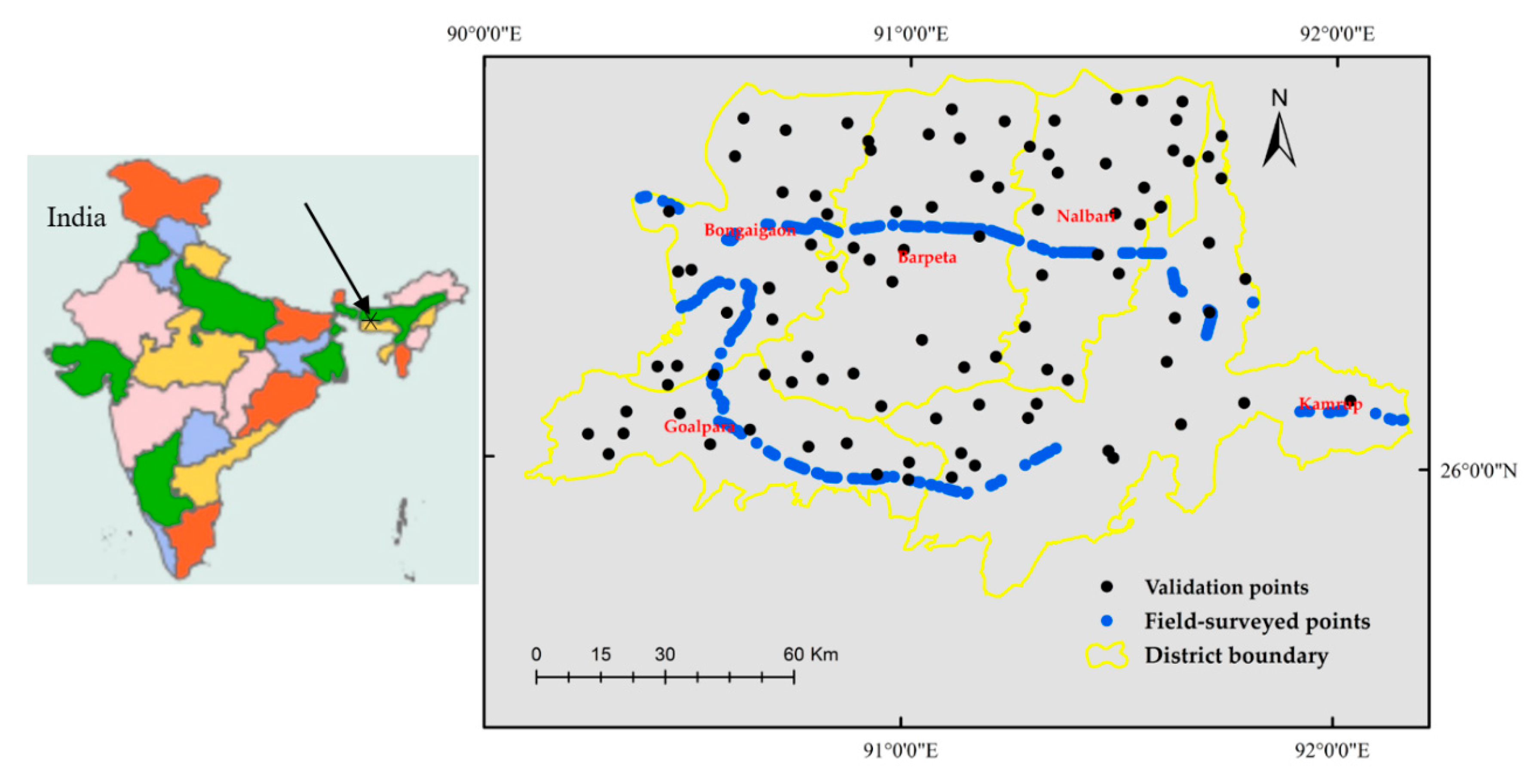
2. Study Area
3. Datasets and Preprocessing
3.1. MODIS Data
3.2. HJ-1A/B Data
3.3. Field Survey Data
3.4. Agriculture Statistics Data
3.5. Ground Reference Data
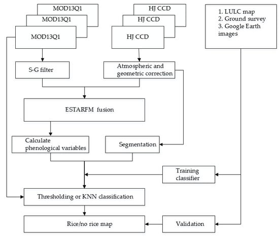
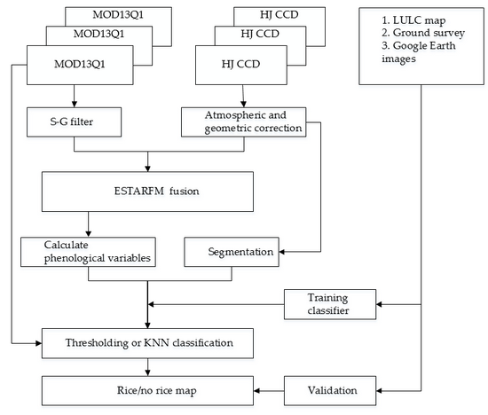
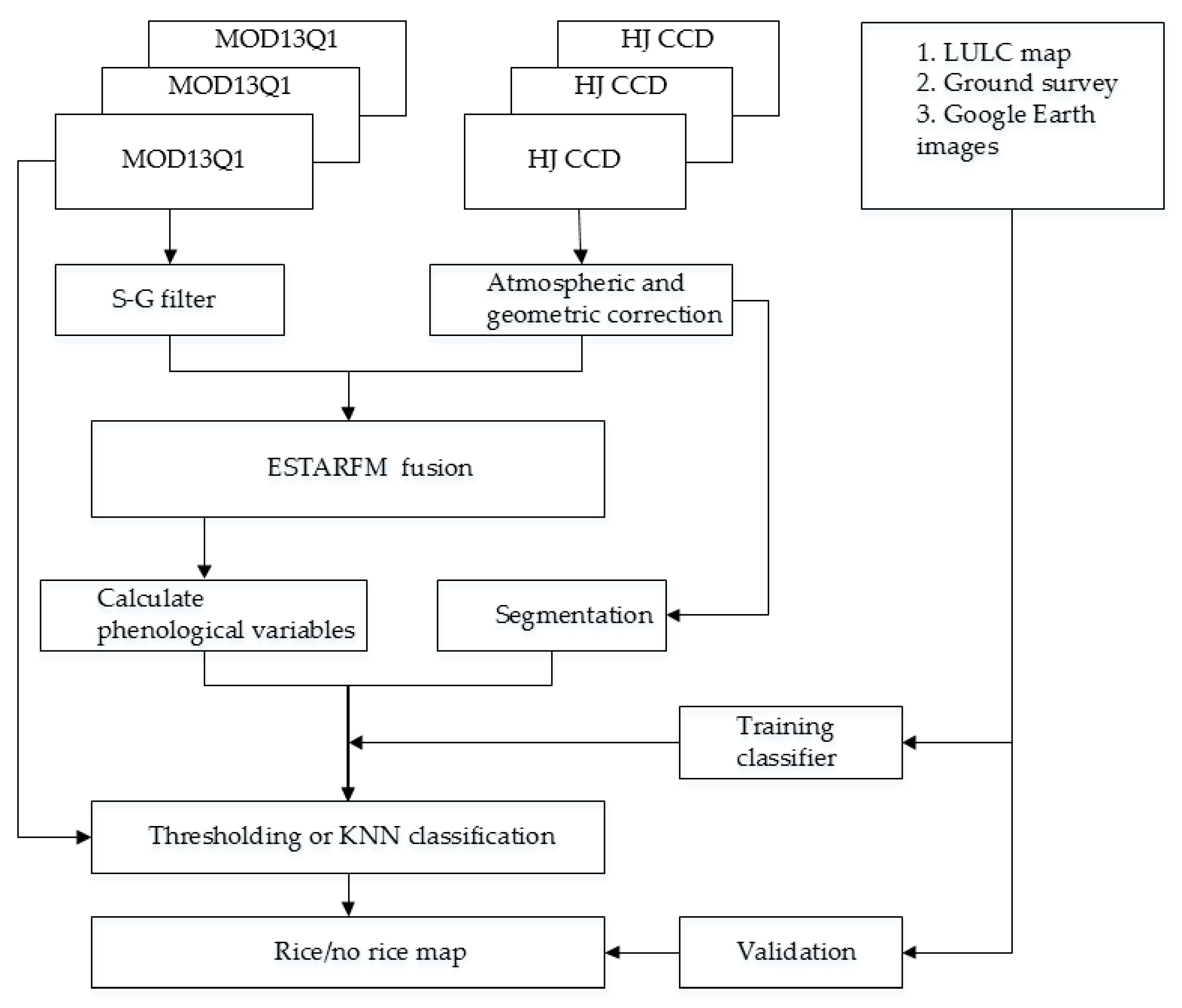
4. Methods
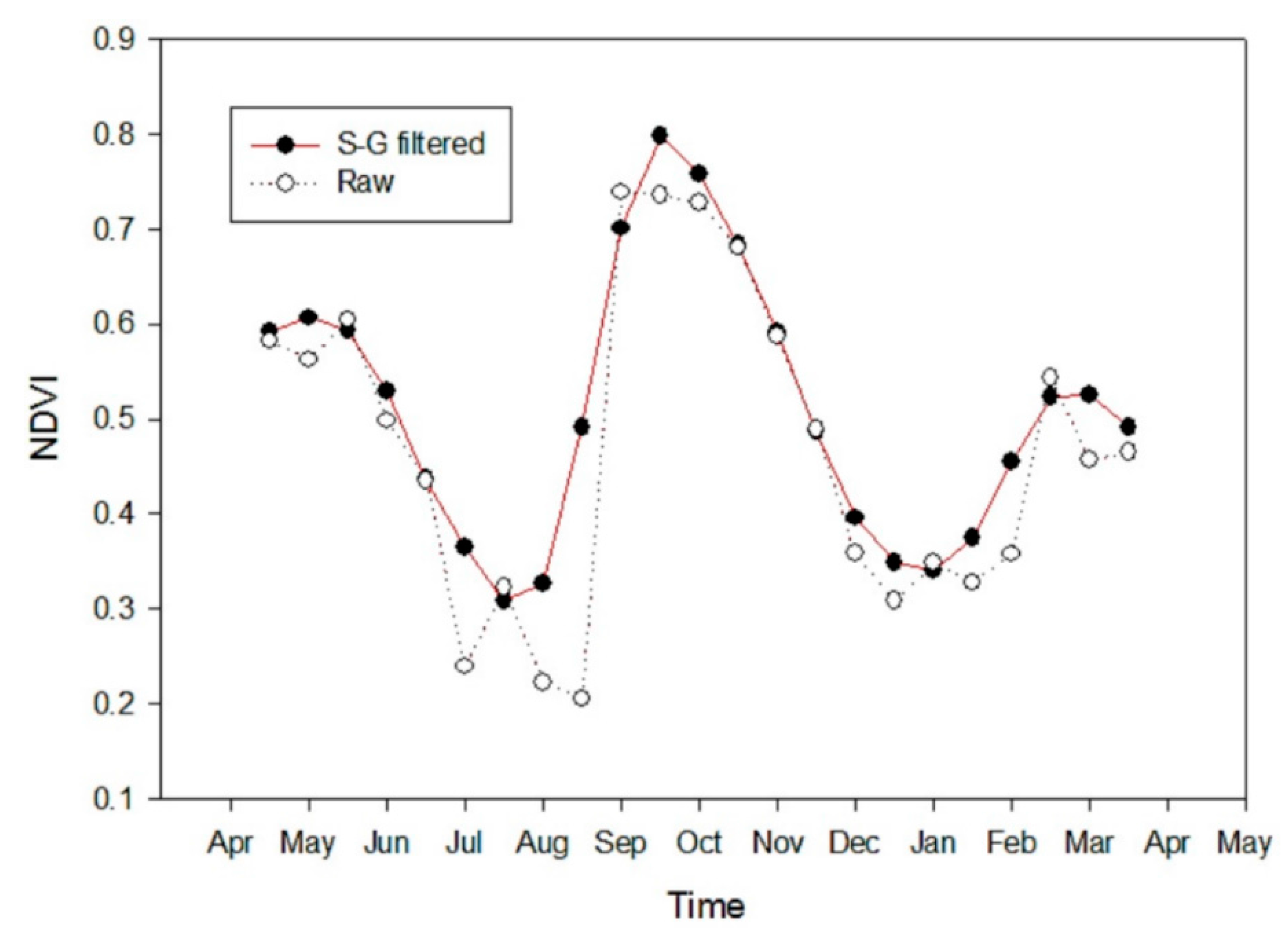
4.1. Construction of Smooth Time Series NDVI
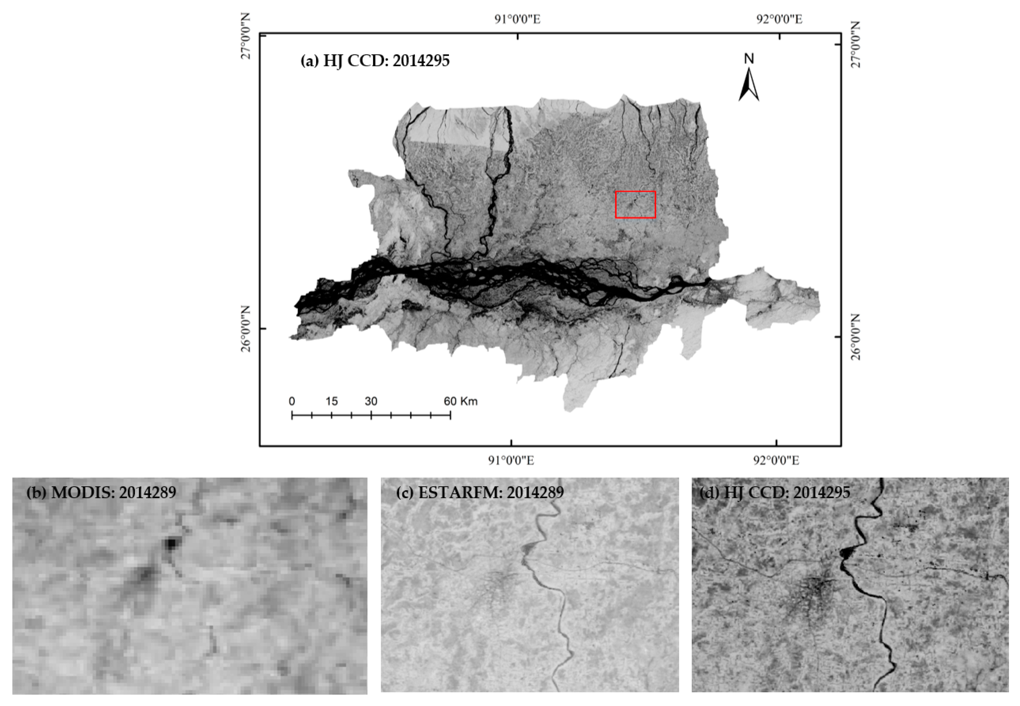
4.2. Blending of Time Series MODIS NDVI and HJ NDVI
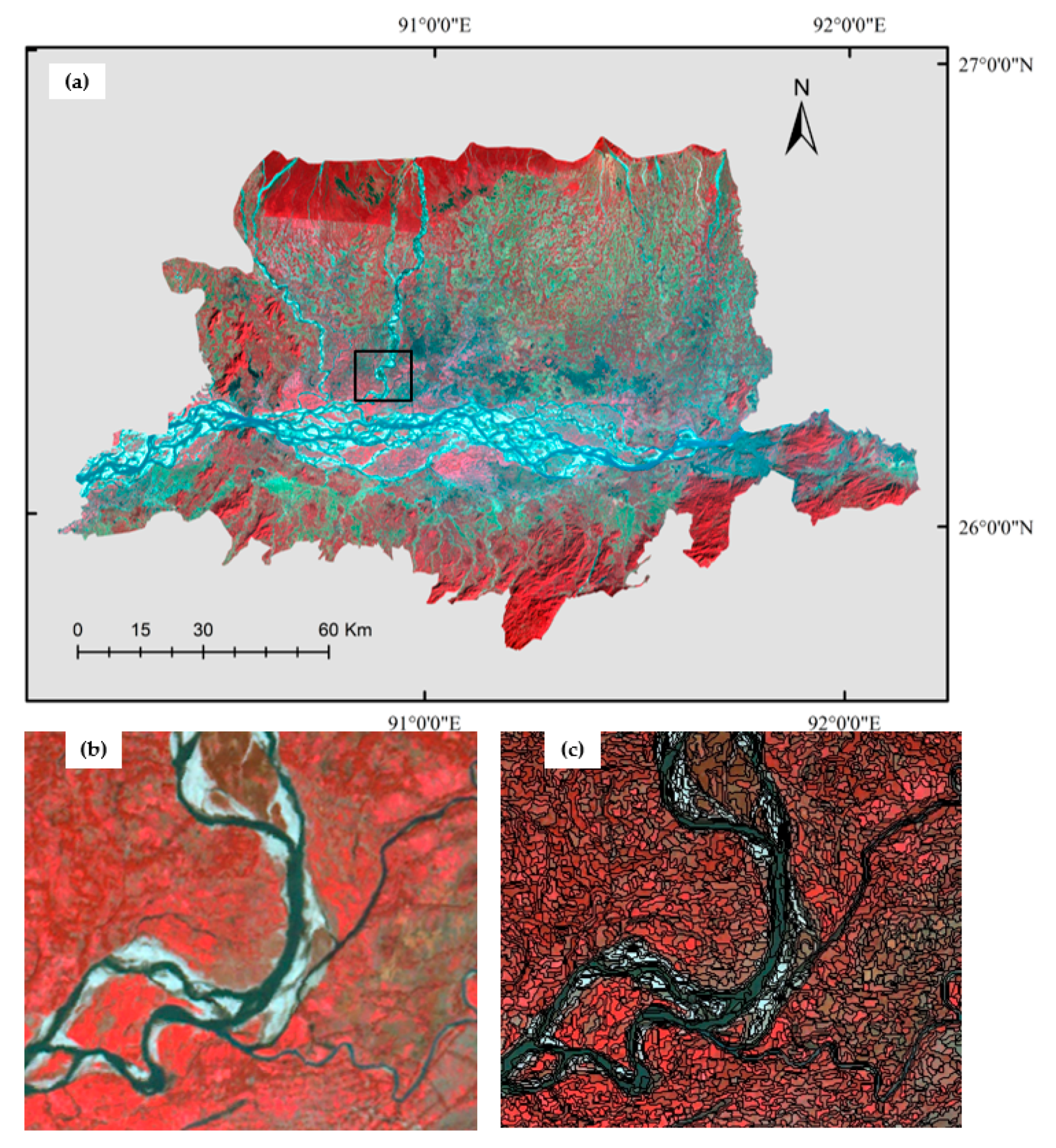
4.3. Image Segmentation and Object Feature Selection
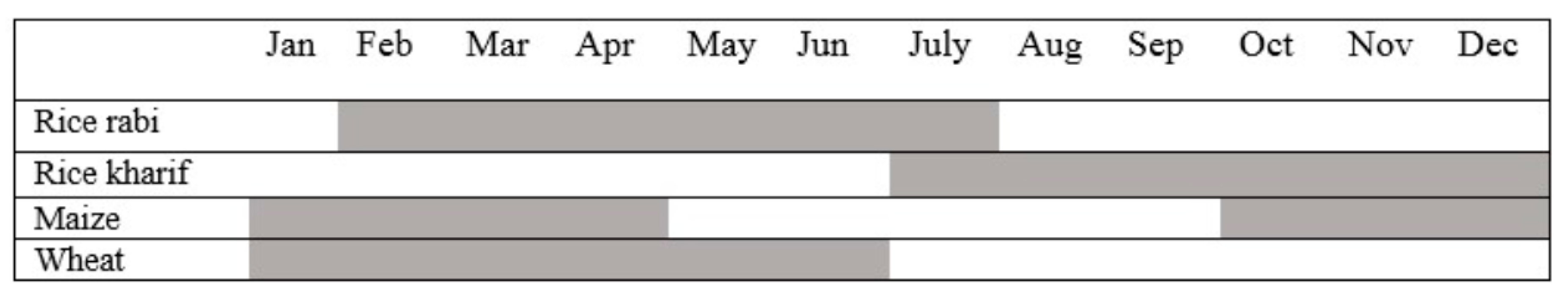
4.4. Derivation of Crop Phenology
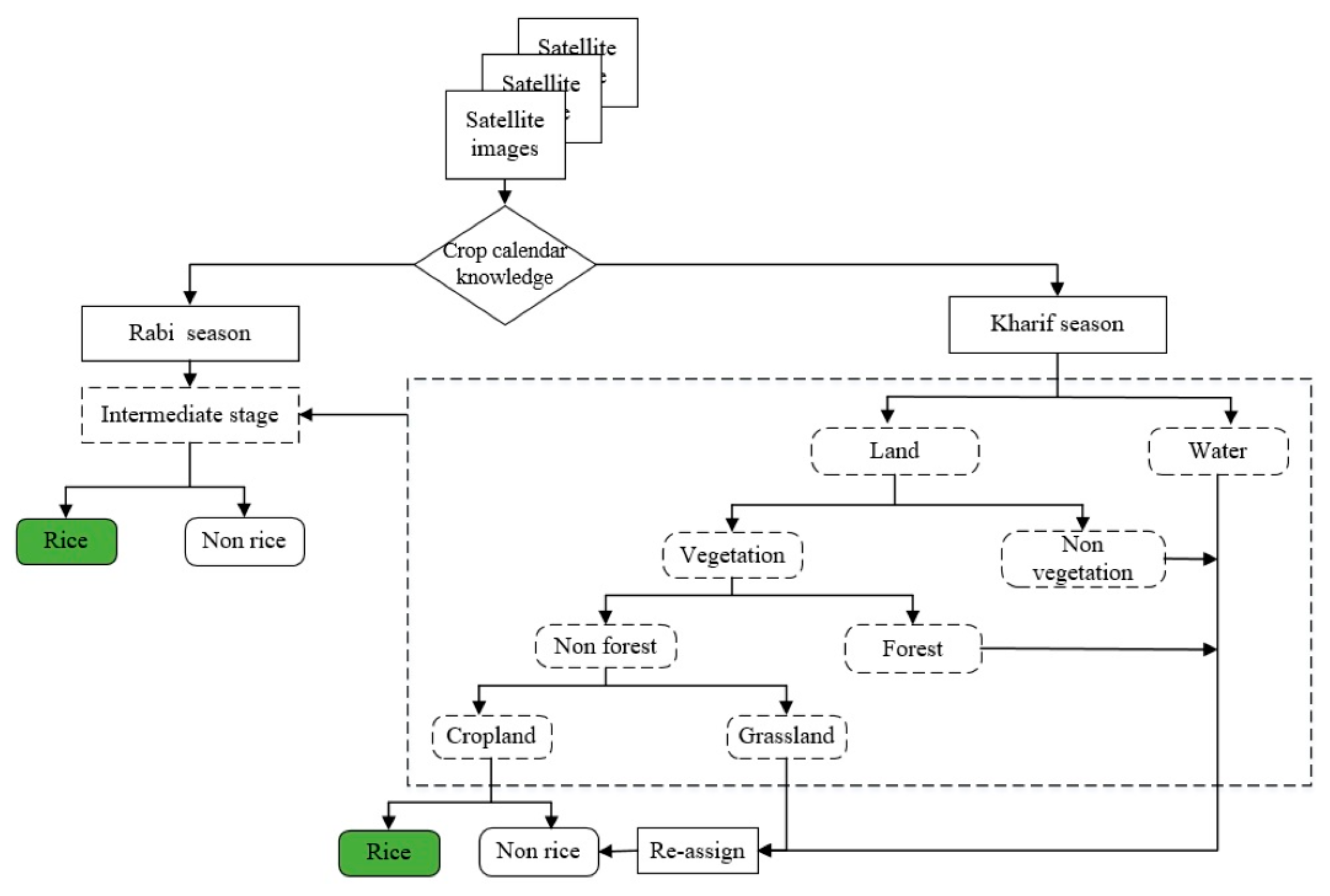
4.5. Classification
4.6. Accuracy Assessment
5. Results
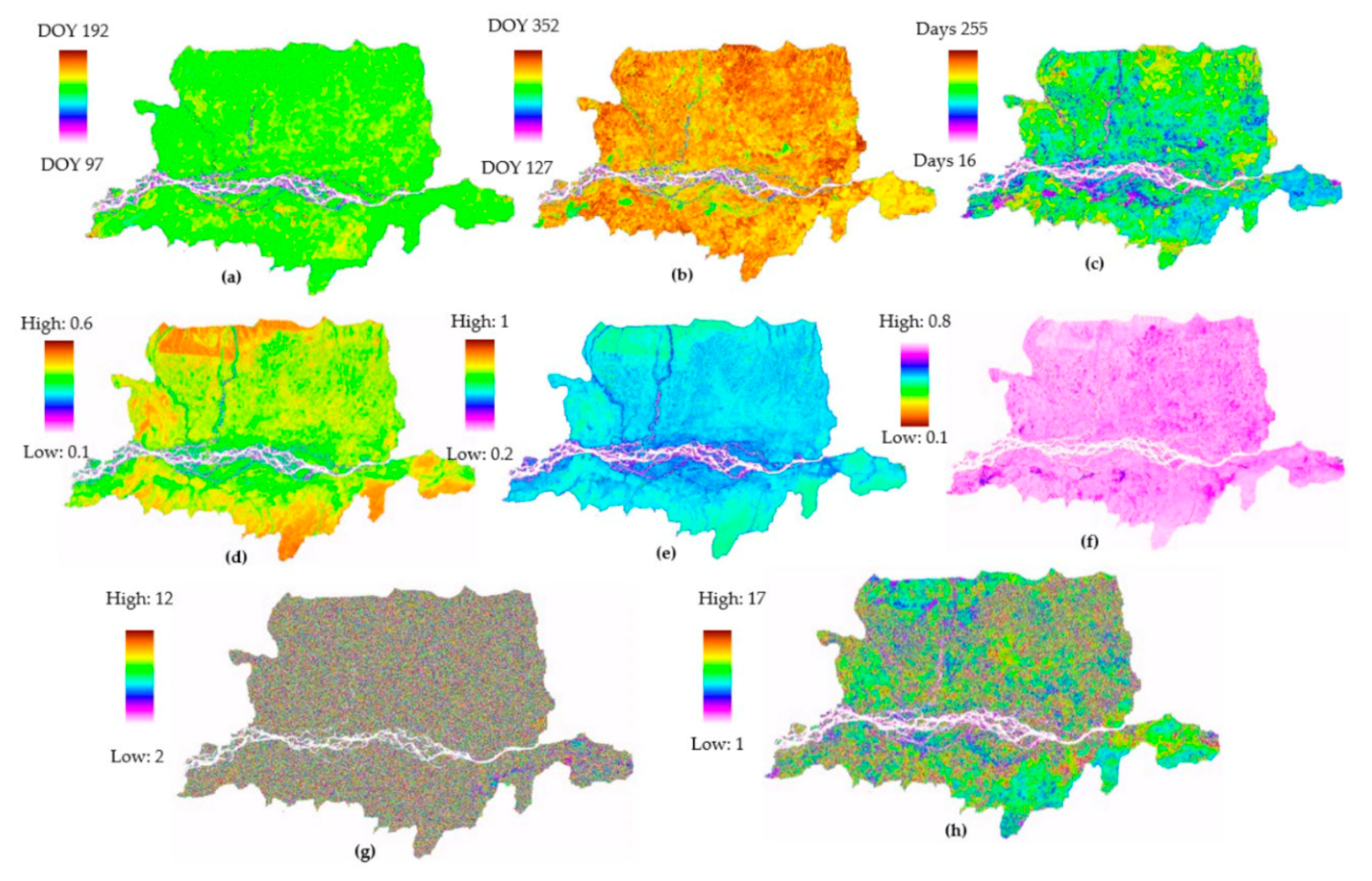
5.1. Phenological Characteristics
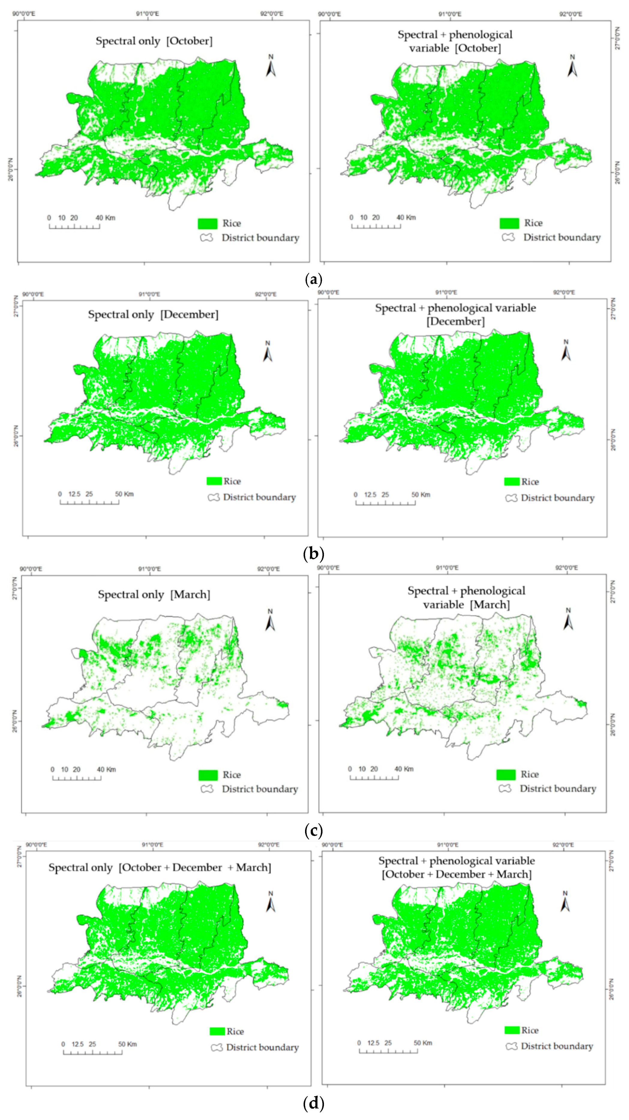
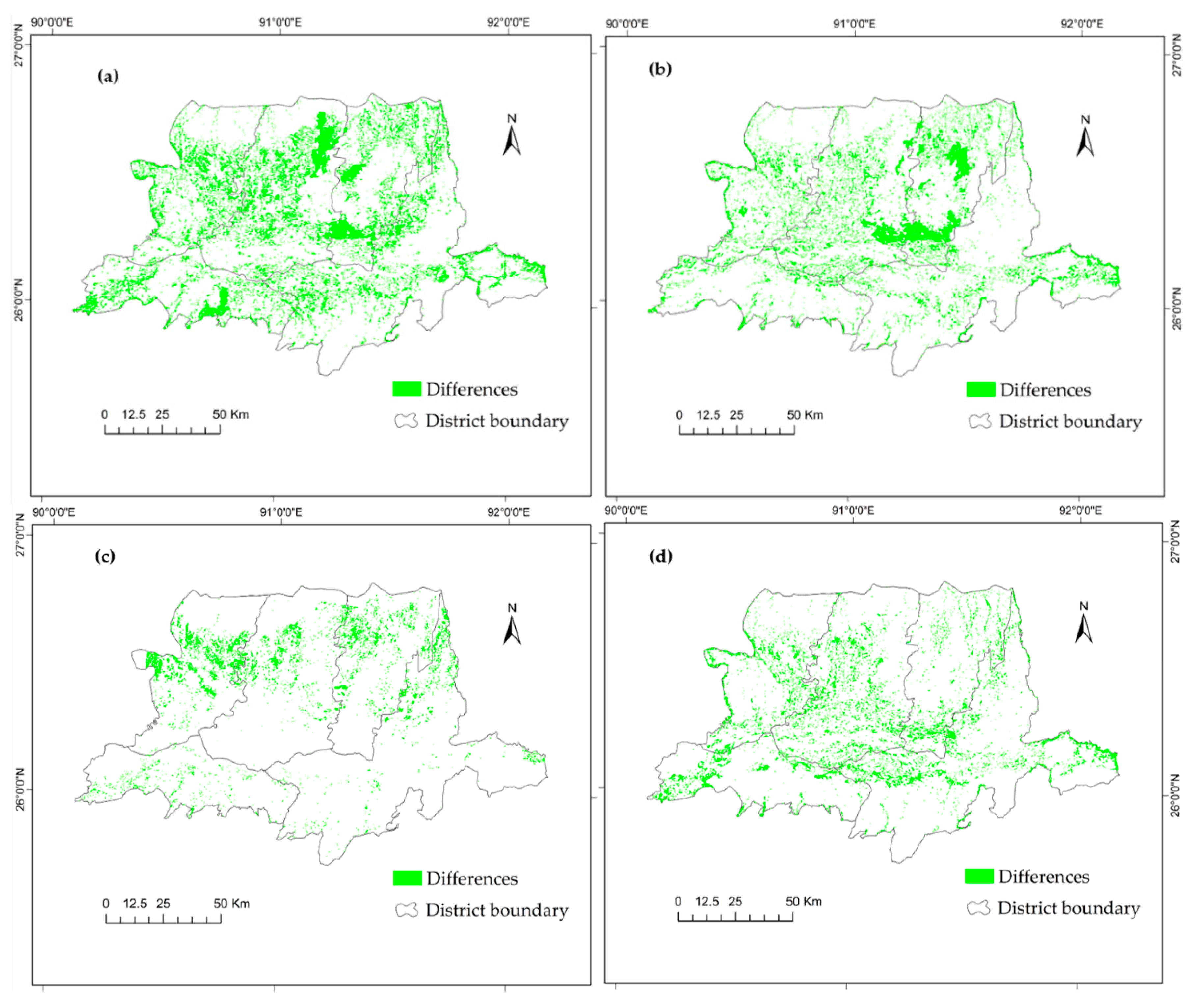
5.2. Identified Rice with and without the Phenological Variables
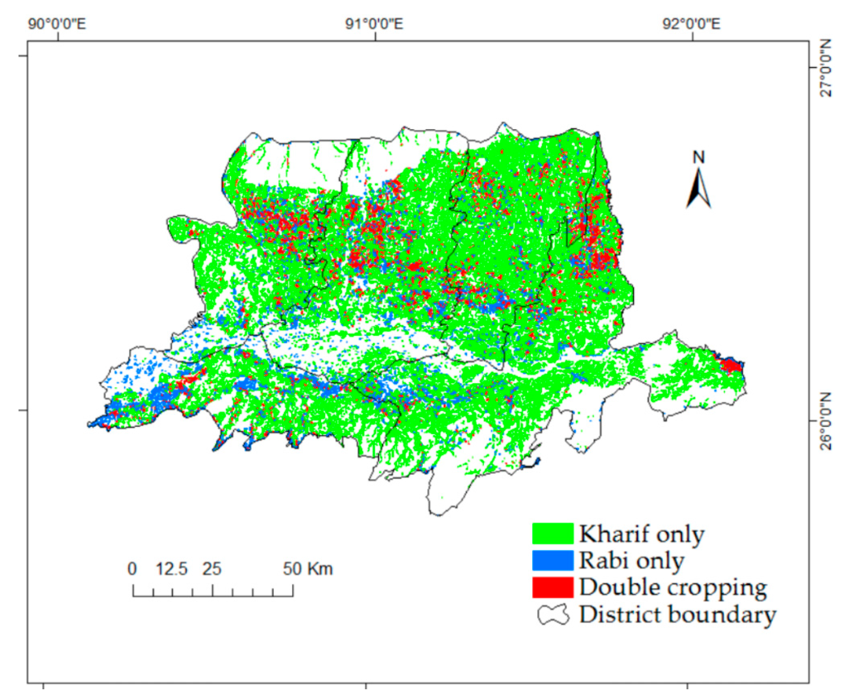
5.3. Spatial Distribution of Rice
5.4. Accuracy Assessment
5.5. Comparison with Agricultural Statistics Data
6. Discussion
7. Conclusions and Future Works
Acknowledgments
Author Contributions
Conflicts of Interest
References
- Maclean, J.; Hardy, B.; Hettel, G. Rice Almanac: Source Book for One of the Most Important Economic Activities on Earth; IRRI: Los Baños, Philippines, 2013. [Google Scholar]
- Bouman, B.A.M.; Humphreys, E.; Tuong, T.P.; Barker, R. Rice and water. Adv. Agron. 2007, 92, 187–237. [Google Scholar]
- Kuenzer, C.; Knauer, K. Remote sensing of rice crop areas. Int. J. Remote Sens. 2013, 34, 2101–2139. [Google Scholar] [CrossRef]
- Nguyen, N.V. Global Climate Changes and Rice Food Security; FAO: Rome, Italy, 2008. [Google Scholar]
- Chen, J.; Huang, J.; Hu, J. Mapping rice planting areas in southern China using the China environment satellite data. Math. Comput. Model. 2011, 54, 1037–1043. [Google Scholar] [CrossRef]
- Fang, H.; Wu, B.; Liu, H.; Huang, X. Using NOAA AVHRR and Landsat TM to estimate rice area year-by-year. Int. J. Remote Sens. 1998, 19, 521–525. [Google Scholar] [CrossRef]
- Gumma, M.K.; Thenkabail, P.S.; Maunahan, A.; Islam, S.; Nelson, A. Mapping seasonal rice cropland extent and area in the high cropping intensity environment of Bangladesh using MODIS 500 m data for the year 2010. ISPRS J. Photogramm. Remote Sens. 2014, 91, 98–113. [Google Scholar] [CrossRef]
- Gumma, M.K.; Mohanty, S.; Nelson, A.; Arnel, R.; Mohammed, I.A.; Das, S.R. Remote sensing based change analysis of rice environments in Odisha, India. J. Environ. Manag. 2015, 148, 31–41. [Google Scholar] [CrossRef] [PubMed]
- Le Toan, T.; Ribbes, F.; Wang, L.-F.; Floury, N.; Ding, K.-H.; Kong, J.A.; Fujita, M.; Kurosu, T. Rice crop mapping and monitoring using ERS-1 data based on experiment and modeling results. IEEE Trans. Geosci. Remote Sens. 1997, 35, 41–56. [Google Scholar] [CrossRef]
- Rossi, C.; Erten, E. Paddy-rice monitoring using TanDEM-X. IEEE Trans. Geosci. Remote Sens. 2015, 53, 900–910. [Google Scholar] [CrossRef]
- Son, N.-T.; Chen, C.-F.; Chen, C.-R.; Duc, H.-N.; Chang, L.-Y. A phenology-based classification of time-series MODIS data for rice crop monitoring in Mekong Delta, Vietnam. Remote Sens. 2013, 6, 135–156. [Google Scholar] [CrossRef]
- Turner, M.D.; Congalton, R.G. Classification of multi-temporal SPOT-XS satellite data for mapping rice fields on a West African floodplain. Int. J. Remote Sens. 1998, 19, 21–41. [Google Scholar] [CrossRef]
- Wang, J.; Xiao, X.; Qin, Y.; Dong, J.; Zhang, G.; Kou, W.; Jin, C.; Zhou, Y.; Zhang, Y. Mapping paddy rice planting area in wheat-rice double-cropped areas through integration of Landsat-8 OLI, MODIS, and PALSAR images. Sci. Rep. 2015, 5. [Google Scholar] [CrossRef] [PubMed]
- Wang, J.; Huang, J.; Zhang, K.; Li, X.; She, B.; Wei, C.; Gao, J.; Song, X. Rice fields mapping in fragmented area using multi-temporal HJ-1A/B CCD images. Remote Sens. 2015, 7, 3467–3488. [Google Scholar] [CrossRef]
- Xiao, X.; Boles, S.; Liu, J.; Zhuang, D.; Frolking, S.; Li, C.; Salas, W.; Moore, B. Mapping paddy rice agriculture in southern China using multi-temporal MODIS images. Remote Sens. Environ. 2005, 95, 480–492. [Google Scholar] [CrossRef]
- Lam-Dao, N. Rice Crop Monitoring Using New Generation Synthetic Aperture Radar (SAR) Imagery. Ph.D. Thesis, University of Southern Queensland, Queensland, Australia, 2009. [Google Scholar]
- Xiao, X.; Boles, S.; Frolking, S.; Li, C.; Babu, J.Y.; Salas, W.; Moore, B. Mapping paddy rice agriculture in South and Southeast Asia using multi-temporal MODIS images. Remote Sens. Environ. 2006, 100, 95–113. [Google Scholar] [CrossRef]
- Gumma, M.K.; Nelson, A.; Thenkabail, P.S.; Singh, A.N. Mapping rice areas of South Asia using MODIS multitemporal data. J. Appl. Remote Sens. 2011, 5. [Google Scholar] [CrossRef]
- Bridhikitti, A.; Overcamp, T.J. Estimation of Southeast Asian rice paddy areas with different ecosystems from moderate-resolution satellite imagery. Agric. Ecosyst. Environ. 2012, 146, 113–120. [Google Scholar] [CrossRef]
- Wan, S.; Lei, T.C.; Chou, T.-Y. An enhanced supervised spatial decision support system of image classification: Consideration on the ancillary information of paddy rice area. Int. J. Geogr. Inf. Sci. 2010, 24, 623–642. [Google Scholar] [CrossRef]
- Chen, C.F.; Chen, C.R.; Son, N.T.; Chang, L.Y. Delineating rice cropping activities from MODIS data using wavelet transform and artificial neural networks in the Lower Mekong countries. Agric. Ecosyst. Environ. 2012, 162, 127–137. [Google Scholar] [CrossRef]
- Qiu, B.; Li, W.; Tang, Z.; Chen, C.; Qi, W. Mapping paddy rice areas based on vegetation phenology and surface moisture conditions. Ecol. Indic. 2015, 56, 79–86. [Google Scholar] [CrossRef]
- Blaschke, T. Object based image analysis for remote sensing. ISPRS J. Photogramm. Remote Sens. 2010, 65, 2–16. [Google Scholar] [CrossRef]
- Kim, H.-O.; Yeom, J.-M. Effect of red-edge and texture features for object-based paddy rice crop classification using RapidEye multi-spectral satellite image data. Int. J. Remote Sens. 2014, 35, 7046–7068. [Google Scholar] [CrossRef]
- Wulder, M.A.; White, J.C.; Hay, G.J.; Castilla, G. Towards automated segmentation of forest inventory polygons on high spatial resolution satellite imagery. For. Chron. 2008, 84, 221–230. [Google Scholar] [CrossRef]
- Dronova, I.; Gong, P.; Wang, L. Object-based analysis and change detection of major wetland cover types and their classification uncertainty during the low water period at Poyang Lake, China. Remote Sens. Environ. 2011, 115, 3220–3236. [Google Scholar] [CrossRef]
- Hellesen, T.; Matikainen, L. An object-based approach for mapping shrub and tree cover on grassland habitats by use of LiDAR and CIR orthoimages. Remote Sens. 2013, 5, 558–583. [Google Scholar] [CrossRef]
- Machala, M.; Zejdová, L. Forest mapping through object-based image analysis of multispectral and LiDAR aerial data. Eur. J. Remote Sens. 2014, 47, 117–131. [Google Scholar] [CrossRef]
- Manjunatha, A.V.; Anik, A.R.; Speelman, S.; Nuppenau, E.A. Impact of land fragmentation, farm size, land ownership and crop diversity on profit and efficiency of irrigated farms in India. Land Use Policy 2013, 31, 397–405. [Google Scholar] [CrossRef]
- Zhu, X.; Chen, J.; Gao, F.; Chen, X.; Masek, J.G. An enhanced spatial and temporal adaptive reflectance fusion model for complex heterogeneous regions. Remote Sens. Environ. 2010, 114, 2610–2623. [Google Scholar] [CrossRef]
- Schmidt, M.; Udelhoven, T.; Gill, T.; Röder, A. Long term data fusion for a dense time series analysis with MODIS and Landsat imagery in an Australian Savanna. J. Appl. Remote Sens. 2012, 6. [Google Scholar] [CrossRef]
- Fenner, M. The phenology of growth and reproduction in plants. Perspect. Plant Ecol. Evol. Syst. 1998, 1, 78–91. [Google Scholar] [CrossRef]
- Esch, T.; Metz, A.; Marconcini, M.; Keil, M. Combined use of multi-seasonal high and medium resolution satellite imagery for parcel-related mapping of cropland and grassland. Int. J. Appl. Earth Obs. Geoinf. 2014, 28, 230–237. [Google Scholar] [CrossRef]
- Zhong, L.; Hawkins, T.; Biging, G.; Gong, P. A phenology-based approach to map crop types in the San Joaquin Valley, California. Int. J. Remote Sens. 2011, 32, 7777–7804. [Google Scholar] [CrossRef]
- Ahmed, T.; Chetia, S.K.; Chowdhury, R.; Ali, S. Status Paper on Rice in Assam: Rice Knowledge Management Portal; Regional Agricultural Research Station: Titabar, India, 2011. [Google Scholar]
- Data Pool | LP DAAC: NASA Land Data Products and Services. Available online: https://lpdaac.usgs.gov/data_access/data_pool (accessed on 1 March 2016).
- Jia, K.; Wu, B.; Li, Q. Crop classification using HJ satellite multispectral data in the North China Plain. J. Appl. Remote Sens. 2013, 7. [Google Scholar] [CrossRef]
- China Resources Satellite Application Center. Available online: http://cresda.com.cn/EN/ (accessed on 1 March 2016).
- Fast Line-of-Sight Atmospheric Analysis of Hypercubes (FLAASH) (Using ENVI) | Exelis VIS Docs Center. Available online: http://www.harrisgeospatial.com/docs/FLAASH.html (accessed on 2 May 2016).
- Wu, B.; Tian, Y.; Li, Q. GVG, a crop type proportion sampling instrument. J. Remote Sens. 2004, 8, 570–580. [Google Scholar]
- Wu, B.; Li, Q. Crop planting and type proportion method for crop acreage estimation of complex agricultural landscapes. Int. J. Appl. Earth Obs. Geoinf. 2012, 16, 101–112. [Google Scholar] [CrossRef]
- Directorate of Economics and Statistics, Assam. Available online: http://ecostatassam.nic.in/ (accessed on 1 March 2016).
- Welcome to Bhuvan | ISRO’s Geoportal | Gateway to Indian Earth Observation. Available online: http://bhuvan.nrsc.gov.in/bhuvan_links.php (accessed on 1 March 2016).
- Welcome to the QGIS Project! Available online: http://qgis.org/en/site/ (accessed on 1 March 2016).
- Chen, J.; Jönsson, P.; Tamura, M.; Gu, Z.; Matsushita, B.; Eklundh, L. A simple method for reconstructing a high-quality NDVI time-series data set based on the Savitzky–Golay filter. Remote Sens. Environ. 2004, 91, 332–344. [Google Scholar] [CrossRef]
- Jarihani, A.A.; McVicar, T.R.; Van Niel, T.G.; Emelyanova, I.V.; Callow, J.N.; Johansen, K. Blending Landsat and MODIS data to generate multispectral indices: A comparison of “Index-then-Blend” and “Blend-then-Index” approaches. Remote Sens. 2014, 6, 9213–9238. [Google Scholar] [CrossRef]
- Definiens, A.G. Definiens eCognition Developer 8 User Guide; Definiens AG: Munchen, Germany, 2009. [Google Scholar]
- Vieira, M.A.; Formaggio, A.R.; Rennó, C.D.; Atzberger, C.; Aguiar, D.A.; Mello, M.P. Object based image analysis and data mining applied to a remotely sensed Landsat time-series to map sugarcane over large areas. Remote Sens. Environ. 2012, 123, 553–562. [Google Scholar] [CrossRef]
- Baatz, M.; Schäpe, A. Multiresolution segmentation: An optimization approach for high quality multi-scale image segmentation. In Proceedings of the Angewandte Geographische Informationsverarbeitung XII, Heidelberg, Germany, January 2000; pp. 12–23.
- Zhang, Y.J. A survey on evaluation methods for image segmentation. Pattern Recognit. 1996, 29, 1335–1346. [Google Scholar] [CrossRef]
- Jönsson, P.; Eklundh, L. TIMESAT—A program for analyzing time-series of satellite sensor data. Comput. Geosci. 2004, 30, 833–845. [Google Scholar] [CrossRef]
- Jonsson, P.; Eklundh, L. Seasonality extraction by function fitting to time-series of satellite sensor data. IEEE Trans. Geosci. Remote Sens. 2002, 40, 1824–1832. [Google Scholar] [CrossRef]
- Reed, B.C.; Brown, J.F.; VanderZee, D.; Loveland, T.R.; Merchant, J.W.; Ohlen, D.O. Measuring phenological variability from satellite imagery. J. Veg. Sci. 1994, 5, 703–714. [Google Scholar] [CrossRef]
- Ruimy, A.; Saugier, B.; Dedieu, G. Methodology for the estimation of terrestrial net primary production from remotely sensed data. J. Geophys. Res. Atmos. 1994, 99, 5263–5283. [Google Scholar] [CrossRef]
- Congalton, R.G.; Green, K. Assessing the Accuracy of Remotely Sensed Data: Principles and Practices; CRC Press: London, UK, 2008. [Google Scholar]
- Tso, B.; Mather, P.M. Classification Methods for Remotely Sensed Data, 2nd ed.; CRC: Boca Raton, FL, USA, 2009. [Google Scholar]
- Leinenkugel, P.; Kuenzer, C.; Oppelt, N.; Dech, S. Characterisation of land surface phenology and land cover based on moderate resolution satellite data in cloud prone areas—A novel product for the Mekong Basin. Remote Sens. Environ. 2013, 136, 180–198. [Google Scholar] [CrossRef]
- Directorate of Economics and Statistics; Govt. of India. Agricultural Statistics at a Glance 2014; Oxford University Press Canada: Don Mills, ON, Canada, 2015.
- Tian, F.; Wang, Y.; Fensholt, R.; Wang, K.; Zhang, L.; Huang, Y. Mapping and evaluation of NDVI trends from synthetic time series obtained by blending Landsat and MODIS data around a coalfield on the Loess Plateau. Remote Sens. 2013, 5, 4255–4279. [Google Scholar] [CrossRef]
- Jia, K.; Liang, S.; Zhang, N.; Wei, X.; Gu, X.; Zhao, X.; Yao, Y.; Xie, X. Land cover classification of finer resolution remote sensing data integrating temporal features from time series coarser resolution data. ISPRS J. Photogramm. Remote Sens. 2014, 93, 49–55. [Google Scholar] [CrossRef]
- Jia, K.; Liang, S.; Wei, X.; Yao, Y.; Su, Y.; Jiang, B.; Wang, X. Land cover classification of Landsat data with phenological features extracted from time series MODIS NDVI data. Remote Sens. 2014, 6, 11518–11532. [Google Scholar] [CrossRef]
- Walker, J.J.; De Beurs, K.M.; Wynne, R.H.; Gao, F. Evaluation of Landsat and MODIS data fusion products for analysis of dryland forest phenology. Remote Sens. Environ. 2012, 117, 381–393. [Google Scholar] [CrossRef]
- Nguyen, T.T.H.; De Bie, C.; Ali, A.; Smaling, E.M.A.; Chu, T.H. Mapping the irrigated rice cropping patterns of the Mekong delta, Vietnam, through hyper-temporal SPOT NDVI image analysis. Int. J. Remote Sens. 2012, 33, 415–434. [Google Scholar] [CrossRef]
- Pan, X.-Z.; Uchida, S.; Liang, Y.; Hirano, A.; Sun, B. Discriminating different landuse types by using multitemporal NDXI in a rice planting area. Int. J. Remote Sens. 2010, 31, 585–596. [Google Scholar] [CrossRef]
- Oguro, Y.; Suga, Y.; Takeuchi, S.; Ogawa, M.; Konishi, T.; Tsuchiya, K. Comparison of SAR and optical sensor data for monitoring of rice plant around Hiroshima. Adv. Space Res. 2001, 28, 195–200. [Google Scholar] [CrossRef]
- Zhang, Y.; Wang, C.; Wu, J.; Qi, J.; Salas, W.A. Mapping paddy rice with multitemporal ALOS/PALSAR imagery in southeast China. Int. J. Remote Sens. 2009, 30, 6301–6315. [Google Scholar] [CrossRef]
- Thenkabail, P.S.; Dheeravath, V.; Biradar, C.M.; Gangalakunta, O.R.P.; Noojipady, P.; Gurappa, C.; Velpuri, M.; Gumma, M.; Li, Y. Irrigated area maps and statistics of India using remote sensing and national statistics. Remote Sens. 2009, 1, 50–67. [Google Scholar] [CrossRef]
- Qin, Y.; Xiao, X.; Dong, J.; Zhou, Y.; Zhu, Z.; Zhang, G.; Du, G.; Jin, C.; Kou, W.; Wang, J. Mapping paddy rice planting area in cold temperate climate region through analysis of time series Landsat 8 (OLI), Landsat 7 (ETM+) and MODIS imagery. ISPRS J. Photogramm. Remote Sens. 2015, 105, 220–233. [Google Scholar] [CrossRef]
- Zhang, G.; Xiao, X.; Dong, J.; Kou, W.; Jin, C.; Qin, Y.; Zhou, Y.; Wang, J.; Menarguez, M.A.; Biradar, C. Mapping paddy rice planting areas through time series analysis of MODIS land surface temperature and vegetation index data. ISPRS J. Photogramm. Remote Sens. 2015, 106, 157–171. [Google Scholar] [CrossRef]
- Teluguntla, P.; Ryu, D.; George, B.; Walker, J.P.; Malano, H.M. Mapping Flooded rice paddies using time series of MODIS imagery in the Krishna River Basin, India. Remote Sens. 2015, 7, 8858–8882. [Google Scholar] [CrossRef]
- Dong, J.; Xiao, X.; Menarguez, M.A.; Zhang, G.; Qin, Y.; Thau, D.; Biradar, C.; Moore, B. Mapping paddy rice planting area in northeastern Asia with Landsat 8 images, phenology-based algorithm and Google Earth Engine. Remote Sens. Environ. 2016. [Google Scholar] [CrossRef]
- Asner, G.P. Cloud cover in Landsat observations of the Brazilian Amazon. Int. J. Remote Sens. 2001, 22, 3855–3862. [Google Scholar] [CrossRef]


| Satellite | Sensor | Acquisition Date |
|---|---|---|
| HJ-1A | CCD2 | 22 October 2014 |
| HJ-1A | CCD1 | 5 December 2014 |
| HJ-1B | CCD1 | 9 March 2015 |
| MODIS | Terra | April 2014–March 2015 |
| Satellite | Sensor | Bands | Wavelength Range (μm) | Spatial Resolution (m) | Swath Width (Km) | Repeat Cycle (Day) |
|---|---|---|---|---|---|---|
| HJ-1A | CCD1 | 1 | 0.43–0.52 | 30 | 360 | 4 |
| CCD2 | 2 | 0.52–0.60 | 30 | |||
| HJ-1B | CCD1 | 3 | 0.63–0.69 | 30 | ||
| CCD2 | 4 | 0.76–0.90 | 30 |
| Phenological Variables | Definition | Meaning |
|---|---|---|
| Start of the season (SOS) | Time for which the left edge has increased to 20% of the seasonal amplitude measured from the left minimum level | Time of start of season |
| End of the season (EOS) | Time for which the right edge has decreased to 20% of the seasonal amplitude measured from the right minimum level | Time of end of season |
| Length of the season (LOS) | Time from the start to the end of the season | Total length of season |
| Base value (BV) | The average of the left and right minimum values | Level of biomass |
| Largest value (LV) | Largest value between the start and end of the season | Level of biomass |
| Seasonal amplitude (SA) | Difference between the maximum value and the base level | Level of biomass |
| Large integral (LI) | Sum of all values from the season start to the end | Net primary production |
| Small integral (SI) | Integral of the difference between the function defining season and the base value | Net primary production |
| Combination of Data | Overall Accuracy | Class | Producer Accuracy | User Accuracy | Kappa |
|---|---|---|---|---|---|
| HJ CCD spectral (October) | 82.00 | Rice | 83.33 | 80.00 | 0.64 |
| Non rice | 80.76 | 84.00 | |||
| HJ CCD spectral (December) | 88.00 | Rice | 86.53 | 90.00 | 0.76 |
| Non Rice | 89.58 | 86.00 | |||
| HJ CCD spectral (March) | 89.00 | Rice | 100.00 | 78.00 | 0.78 |
| Non Rice | 81.96 | 100.00 | |||
| HJ CCD Spectral (October, December, March) | 89.00 | Rice | 88.23 | 90.00 | 0.78 |
| Non Rice | 89.79 | 88.00 | |||
| HJ CCD Spectral (October) + PV | 84.00 | Rice | 85.41 | 82.00 | 0.68 |
| Non Rice | 82.69 | 86.00 | |||
| HJ CCD Spectral (December) + PV | 90.00 | Rice | 90.00 | 90.00 | 0.80 |
| Non Rice | 90.00 | 90.00 | |||
| HJ CCD Spectral (March) + PV | 91.00 | Rice | 100.00 | 82.00 | 0.82 |
| Non Rice | 84.74 | 100.00 | |||
| HJ CCD Spectral (October, December, March) + PV | 93.00 | Rice | 92.15 | 94.00 | 0.86 |
| Non Rice | 93.87 | 92.00 |
| Districts | Estimated (2014–2015) | Statistics (2012–2013) | Difference (%) |
|---|---|---|---|
| Barpeta | 68.93 | 119.51 | −53.68 |
| Bongaigaon | 51.22 | 46.67 | 9.31 |
| Goalpara | 45.89 | 74.2 | −47.13 |
| Kamrup | 78.08 | 131.94 | −51.29 |
| Nalbari | 72.27 | 76.13 | −5.19 |
| Total | 316.39 | 448.45 | −34.53 |
| Reference | Approach | Study Area |
|---|---|---|
| Xiao et al. [15,17] | (1) Based on the relationships between LSWI and NDVI/EVI during flooding and transplanting time | South Asia, Southeast Asia and Southern China |
| (2) Timing of flooding and transplanting: all 8-day composites in one year | ||
| Zhang et al. [69] | (1) Based on the relationships between LSWI and NDVI/EVI during flooding and transplanting time | Northeastern China |
| (2) Timing of flooding and transplanting: between the date of LST (land surface temperature) 5 °C and EVI = 0.35 | ||
| Teluguntla et al. [70] | (1) Based on the relationships between LSWI and NDVI/EVI during flooding and transplanting time | Krishna River basin, India |
| (2) Timing of flooding and transplanting: according to the calendars of 2000–2010 | ||
| Qiu et al. [22] | (1) Based on the relationships between LSWI and EVI2 (Enhanced Vegetation Index 2) during tillering and heading time | Southern China |
| (2) Timing of tillering and heading: according to EVI2 temporal profiles | ||
| This study | (1) Based on the combined use of crop phenology and spectral data | Assam, India |
| (2) Phenology extraction: according to NDVI temporal profiles |
© 2016 by the authors; licensee MDPI, Basel, Switzerland. This article is an open access article distributed under the terms and conditions of the Creative Commons Attribution (CC-BY) license (http://creativecommons.org/licenses/by/4.0/).
Share and Cite
Singha, M.; Wu, B.; Zhang, M. An Object-Based Paddy Rice Classification Using Multi-Spectral Data and Crop Phenology in Assam, Northeast India. Remote Sens. 2016, 8, 479. https://doi.org/10.3390/rs8060479
Singha M, Wu B, Zhang M. An Object-Based Paddy Rice Classification Using Multi-Spectral Data and Crop Phenology in Assam, Northeast India. Remote Sensing. 2016; 8(6):479. https://doi.org/10.3390/rs8060479
Chicago/Turabian StyleSingha, Mrinal, Bingfang Wu, and Miao Zhang. 2016. "An Object-Based Paddy Rice Classification Using Multi-Spectral Data and Crop Phenology in Assam, Northeast India" Remote Sensing 8, no. 6: 479. https://doi.org/10.3390/rs8060479
APA StyleSingha, M., Wu, B., & Zhang, M. (2016). An Object-Based Paddy Rice Classification Using Multi-Spectral Data and Crop Phenology in Assam, Northeast India. Remote Sensing, 8(6), 479. https://doi.org/10.3390/rs8060479