Article

First in-Flight Radiometric Calibration of MUX and WFI on-Board CBERS-4

1
Division of Remote Sensing, National Institute for Space Research—INPE, 12227-010 São José dos Campos, Brazil
2
Division of Geointelligence (EGI), Institute for Advanced Studies—IEAv/CTA, 12231-970 São José dos Campos, Brazil
3
Division of Mathematics and Physics, Universidade de Taubaté—UNITAU, 12201-970 Taubaté, Brazil
4
Office of Engineering Research, College of Engineering, South Dakota State University, Brookings, SD 57007, USA
*
Author to whom correspondence should be addressed.
Remote Sens. 2016, 8(5), 405; https://doi.org/10.3390/rs8050405
Submission received: 3 February 2016 / Revised: 5 April 2016 / Accepted: 5 May 2016 / Published: 11 May 2016

Abstract

:
Brazil and China have a long-term joint space based sensor program called China-Brazil Earth Resources Satellite (CBERS). The most recent satellite of this program (CBERS-4) was successfully launched on 7 December 2014. This work describes a complete procedure, along with the associated uncertainties, used to calculate the in-flight absolute calibration coefficients for the sensors Multispectral Camera (MUX) and Wide-Field Imager (WFI) on-board CBERS-4. Two absolute radiometric calibration techniques were applied: (i) reflectance-based approach and (ii) cross-calibration method. A specific site at Algodones Dunes region located in the southwestern portion of the United States of America was used as a reference surface. Radiometric ground and atmospheric measurements were carried out on 9 March 2015, when CBERS-4 passed over the region. In addition, a cross-calibration between both MUX and WFI on-board CBERS-4 and the Operational Land Imager (OLI) on-board Landsat-8 was performed using the Libya-4 Pseudo Invariant Calibration Site. The gain coefficients are now available: 1.68, 1.62, 1.59 and 1.42 for MUX and 0.379, 0.498, 0.360 and 0.351 for WFI spectral bands blue, green, red and NIR, respectively, in units of (W/(m2·sr·μm))/DN. These coefficients were determined with uncertainties lower than 3.5%. As a validation of these radiometric coefficients, cross-calibration was also undertaken. An evaluation of radiometric consistency was performed between the two instruments (MUX and WFI) on-board CBERS-4 and with the well calibrated Landsat-7 ETM+. Results show that the reflectance values match in all the analogous spectral bands within the specified calibration uncertainties.

Graphical Abstract

1. Introduction

The incorporation of Brazil into a long-term remote sensing program has begun with the establishment of the China Brazil Earth Resources Satellite (CBERS) program. The CBERS program has been developed under a cooperation agreement between Brazil and China [1]. The first satellite (CBERS-1) developed was launched on 14 October 1999 by the Chinese Long March 4B launcher from the Taiyuan Satellite Launch Center in China [1]. CBERS-1 remained functional until August 2003. The second satellite (CBERS-2) was launched successfully from the same launch center on 21 October 2003 and carried an identical instrument set as CBERS-1.
In 2002, the governments of China and Brazil decided to expand the initial agreement to include the construction of two new additional satellites: CBERS-3 and CBERS-4 as the second generation of the Chinese-Brazilian cooperation effort [2]. In 2004, a new agreement was signed to build the CBERS-2B, which was launched before CBERS-3, in 2007 and operated until June 2010. The agreement for CBERS-2B was made based on concern of a possible interruption in data acquisition. Unfortunately, despite this agreement and successful operation of CBERS-2B, there was a significant interruption of data acquisition while awaiting the launch of the CBERS-3 and 4 series of sensors.
CBERS-3 was launched in 9 December 2013, also by a Long-March 4B rocket from the Taiyuan base in China; however, the satellite was lost due to a failure on the launcher’s third stage. The launch of CBERS-4 was originally scheduled for December 2015. However, due to the loss of the CBERS-3 satellite, China and Brazil agreed to accelerate the launch schedule. On 7 December 2014, the CBERS-4 was successfully launched from the Taiyuan Satellite Launch Center.
CBERS-4 carries four cameras in the payload module [3]: (a) Panchromatic and Multispectral Camera (PAN); (b) Multispectral Camera (MUX); (c) Infrared System (IRS); (d) Wide-Field Imager (WFI). Brazil is responsible for both MUX and WFI cameras, while China is responsible for the IRS and PAN. This responsibility division extends to other systems and also the cost of the entire mission, which is 50% for each country [3].
The success of any remote sensing program depends on the knowledge of the radiometric properties of the sensor from which the data will be available [4]. A great example of that is the Landsat series of satellites, whose radiometric characteristics have been evaluated and updated continuously [5,6,7,8]. The radiometric calibration, from pre-launch through end-of-mission, permits users to apply the data as a true quantitative input to Earth study applications.
In conjunction with absolute radiometric calibration, it is essential to have a firm quantitative understanding of the uncertainty of this calibration. This work describes a complete procedure, along with the associated uncertainties, used to calculate the in-flight absolute calibration coefficients for MUX and WFI level 1 images. For this purpose two absolute radiometric calibration techniques were used: (i) reflectance-based approach and (ii) cross-calibration method.
The reflectance-based approach has been widely used with success for orbital sensors [9,10,
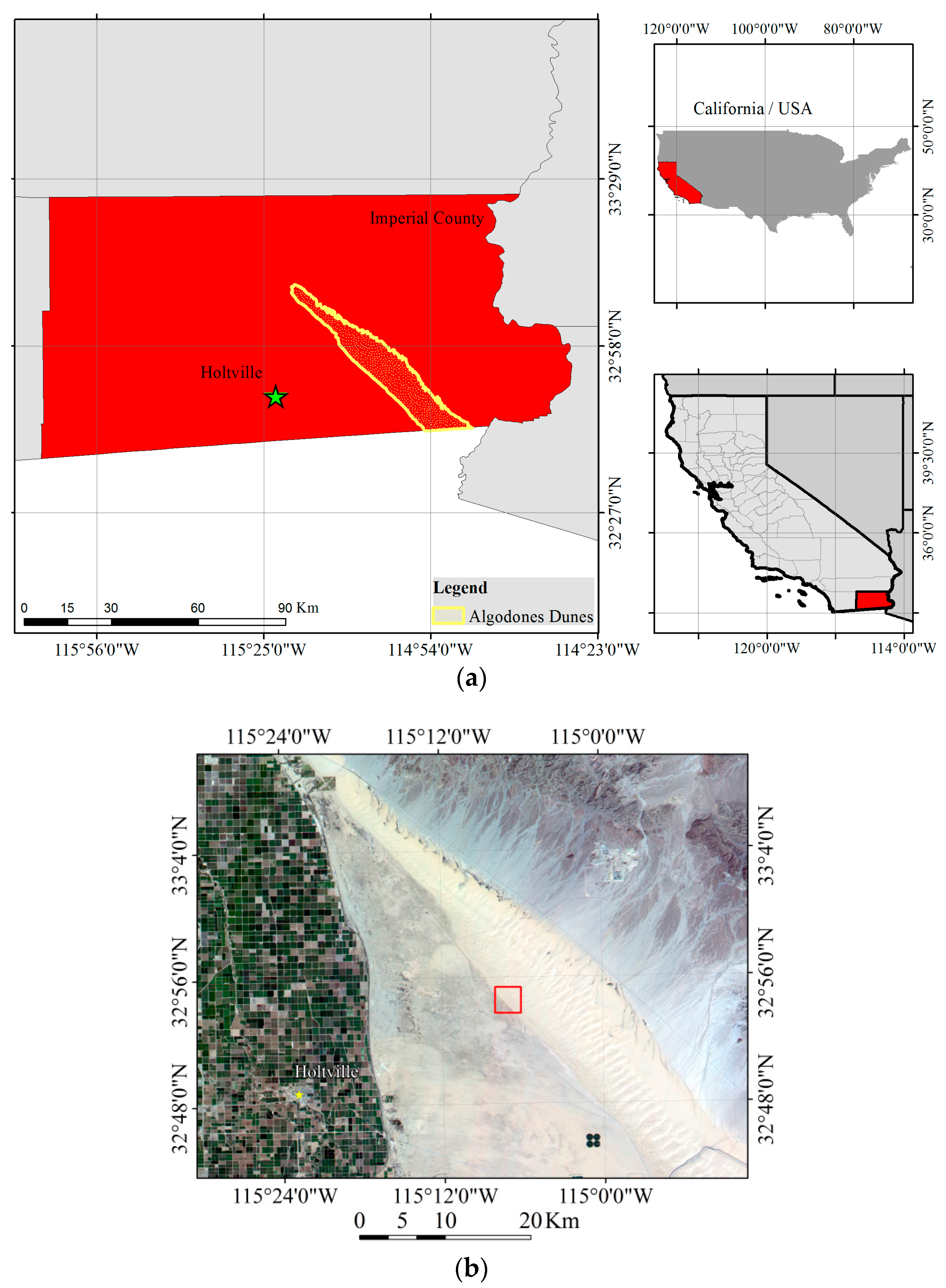
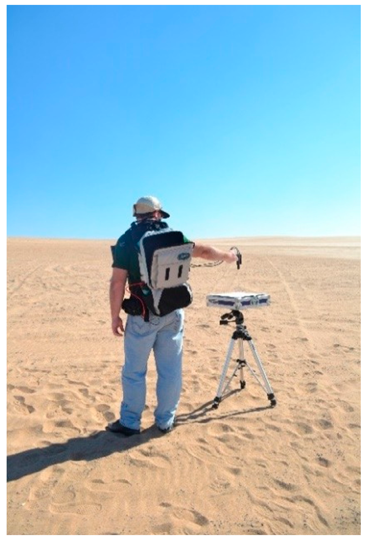
11]. This method uses the reflectance-based ground truth measurement of a test site (reference surface) along with atmospheric measurement during an overpass of the reference surface by the sensor. The data derived from ground measurement are utilized as input to a radiative transfer code to predict the radiance/reflectance values at sensor (top of atmosphere radiance/reflectance). The predicted at sensor radiance is then compared with the DN count from the sensor to obtain the calibration coefficient for each sensor spectral band. Here, an area at Algodones Dunes region located in the southwestern portion of the United States of America, California, was used as a reference surface.
Whereas for the cross-calibration method the calibration is transferred from a radiometrically well-characterized reference sensor, whose calibration accuracy is known, to a target sensor using near-simultaneous ground observations [12]. The MUX and WFI on-board CBERS-4 was cross calibrated with the newest Landsat series sensor OLI (Operational Land Imager). This calibrated was performed based on imaging of the Libya-4 Pseudo Invariant Calibration Site (PICS) [13,14,15,16]. PICS have been used primarily for sensor radiometric stability monitoring, for the purpose of detecting changes in absolute radiometric accuracy [14].
Additionally, the calibration coefficients have been validated using the cross-calibration technique. Evaluation of the radiometric consistency between both MUX and WFI sensors on-board CBERS-4 and the well calibrated over time Landsat-7 Enhanced Thematic Mapper Plus (ETM+) was performed. The comparison was based on cross-calibration between the three orbital sensors using image pairs from Algodones Dunes.

2. CBERS-4: MUX and WFI

The CBERS-4 satellite has a sun-synchronous orbit with an altitude of 778 km. The local solar time at the equator crossing is always 10:30 a.m. The CBERS-4 incorporates an on-board radiometric calibration system. However, there remains uncertainty in terms of the engineering of the internal calibration system control. Due to this fact, the vicarious calibration performed in this work is even more important.
MUX/CBERS-4 is a multispectral camera with four spectral bands covering the wavelength range from blue to near infrared (450 nm to 890 nm) with a ground resolution of 20 m and a ground swath width of 120 km. The main function of the MUX is to maintain continuity with the previous CBERS sensors [3]. It is the sensor which ensures global coverage at a standard spatial resolution every 26 days.
WFI/CBERS-4 had a significant improvement in characteristics compared to previous WFI sensor. WFI is also a multispectral camera, featuring four spectral bands covering the range of wavelengths from blue to near infrared. Its ground resolution is 64 m at nadir, without losing the revisit capacity of five days, due to the large Field of View of ±28.63°. Table 1 shows a summary of the MUX and WFI characteristics. 
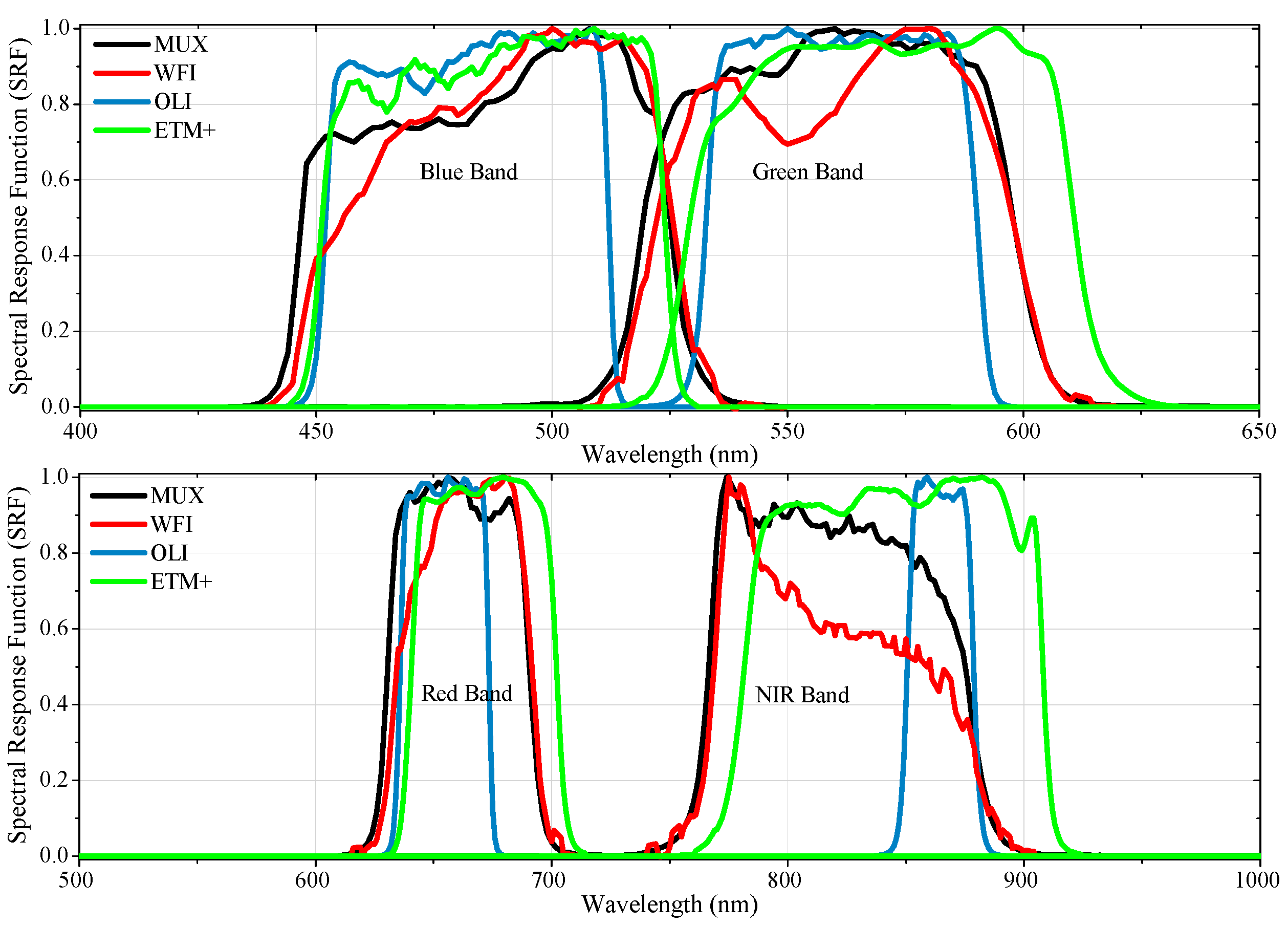
Figure 1 shows the MUX and WFI Spectral Response Function (SRF) profiles. For comparison purposes, Figure 1 also presents the Landsat-8/OLI and Landsat-7/ETM + SRF.
The relationship between Digital Number (DN) acquired from the sensor and TOA radiance in each spectral band of the MUX and WFI was established by the equation below:
L i = G i × D N i + o f f s e t i
where: Li is the TOA radiance at band i in units of (W/(m2·sr·μm)); DNi is the digital number from the image at band i; Gi is the coefficient gain for band i in units of (W/(m2·sr·μm))/DN; and offseti is the coefficient bias for band i in units of (W/(m2·sr·μm)). This work will describes the procedure to calculate Gi and offseti for both sensors MUX and WFI on-board CBERS-4.
The MUX and WFI image radiance data can then be converted to planetary TOA reflectance data using the conversion equation:
ρ λ = π L λ d 2 E S U N λ cos θ z
where: ρλ is the planetary TOA reflectance (unitless); π is the mathematical constant (unitless); Lλ is the spectral radiance at the sensor’s aperture (W/(m2·sr·μm)); d is the Earth-Sun distance (astronomical units); θz is the solar zenith angle (degrees or radians); and ESUNλ is mean exoatmospheric solar irradiance (W/(m2·μm)).
The mean exoatmospheric solar irradiance, ESUNλ, for MUX and WFI sensors was estimated using the CHKUR Extraterrestrial Solar Spectral Irradiance dataset from MODTRAN 5.2.1 software. It is important to note that an estimate of the ESUNλ at each spectral band of MUX and WFI is incomplete unless accompanied with uncertainty. The accuracy of the solar spectrum was considered within 1%–2%, then, this uncertainty was propagated (using the Monte Carlo technique described in Section 6) to the mean solar exoatmospheric irradiance of each sensor spectral band. The ESUNλ values for MUX and WFI spectral bands are summarized in Table 2.

3. Reflectance-Based Approach

The reflectance-based approach requires an accurate field radiometric measurement concurrent with the overpass of the sensor. The ground based radiometric measurements involve two distinct types of measurements: one for determination of the surface radiance (or reflectance) and the other to characterize the atmosphere. The data derived from ground measurements are used as input in a radiative transfer code to predict the radiance/reflectance values at sensor (top of atmosphere radiance). These results are then compared to the digital number reported by the sensor to provide a set of bias and gains for the sensor bands (radiometric calibration coefficients).

3.1. Field Campaign

On 9–13 March 2015, a joint field campaign was conducted at the Imperial Sand Dunes Recreation Area (commonly referred to as Algodones Dunes) and involved five different teams: Arizona Remote Sensing Group (RSG), South Dakota State University (SDSU), Rochester Institute of Technology (RIT), University of Lethbridge and Goddard Space Flight Center (GSFC). The SDSU team collected the data used in this work.
Algodones Dunes is located in the southwestern portion of the United States of America, in the state of California at latitude 32°54′ N and longitude 115°07′ W (Figure 2a). The area provides positive characteristics for calibration purposes, including high-reflectance, sufficiently large size, low amount of atmospheric aerosols, good temporal stability, sufficient spatial stability, and easy access. The CBERS-4 overpassed the region on 9 March 2015; therefore, the data collected in this date were used in this work. Figure 2b is the MUX/CBERS 4 image of the region.

3.2. Surface Reflectance

Reflectance is the ratio of the total amount of electromagnetic radiation (EM) reflected by a surface to the total amount of EM incident on the surface [17,18]. However, reflectance cannot be measured directly, because the infinitesimal elements of the solid angle do not include measurable amounts of radiant flux [19]. Thus, due to technical difficulties measuring reflectance in either field measurements or laboratory, the reflectance factor (RF) is the equivalent used in practice [20]. This quantity is the ratio of spectral radiance reflected from a sample (target) to the spectral radiance that would be reflected by a perfect diffuse Lambertian surface, under the same geometry conditions, according to Equation (3) [20]. In practice, a perfectly reflecting panel does not exist; therefore, a correction is made to account for the spectral reflectance panel.
R F t a r g e t = L t a r g e t L p a n e l × k
where: Ltarget is the radiance of the target, Lpanel is the radiance of the reference panel under the same illumination and view geometry; and k is the panel correction factor. The panel correction factor is usually calibrated by the supplier, or as was the case in this campaign; calibrated by Arizona Remote Sensing Group (RSG).
A 160 by 300 m surface with 18 uniformly positioned sample points was selected at Algodones Dunes. The size of the reference surface is chosen based on the spatial resolution of the sensor, i.e., the size of the chosen site must be compatible with the pixel size of the sensor you desire calibrate. For ETM+/Landsat-7, TM/Landsat 4 and 5, for example, the sites were a rectangular area that is 480 by 120 m [10]. The size of one site used to calibrate the OLI/Landsat-8 was 100 by 250 m [21]. Here, a 160 by 300 m surface was selected, which is appropriate size to calibrate sensors on-board CBERS-4 (or better ground spatial resolution). Furthermore, making the size of the text site larger would provide more statistical sampling, but increasing the size also causes the data collection to take longer. This can generate more uncertainty due to changes in solar zenith angle causing bidirectional reflectance effects and increases the probability of changes in atmospheric conditions [10].
The surface reflectance was measured using a FieldSpec Pro hyperspectral spectroradiometer from ASD (Analytical Spectral Devices) [22], which cover the wavelength range from 350 nm through 2500 nm. A Spectralon panel from Labsphere [23] was used as the approximate ideal diffuse standard surface. The panel reflectance (panel correction factor from Equation (3)) is known as a function of angle and wavelength [24]. The FieldSpec ASD was operated only by hand with the collection unit held vertically toward the ground (about 1.3 m high), with the operator avoiding the projection of his shadow on the area measured. The FieldSpec ASD was configured to average 20 spectra per sample and it was transported across the area using a backpack device (Figure 3).
The reference panel was kept on a tripod near the sample point in a horizontal position (Figure 3). At the beginning of each data acquisition the FieldSpec ASD was optimized and five sample spectra of the reference panel were acquired. Next, approximately 17 averaged sample spectra of the target (reference surface) were obtained by walking in line until the next point. Then, the reference panel was again viewed by the FieldSpec ASD and five sample spectra were obtained. This procedure was performed in all 18 set points over a period of 1 h.

3.3. Atmospheric Characterization

The atmospheric characterization data were collected at the same time as the surface reflectance measurements. The atmospheric characterization was performed using an Automated Solar Radiometer (ASR) developed and manufactured by the University of Arizona running in ten spectral bands [25]. The ASR generates a digital output signal which is linearly proportional to the solar irradiance. This can be modeled according to the Beer Law [26,27,28].
Assuming that total optical depth remains constant over the range of air masses for which measurements are performed, a Langley plot (linearization of Beer’s law) will yield a set of data points distributed along a straight line with slope equal to the total optical depth and intercept equal the natural logarithm of the ASR calibration constant [26,27,28].
Absorption by water vapor is restricted to narrow spectral bands. Therefore, the spectral range centered approximately at 940 nm was used to estimate the water vapor atmospheric content. Columnar water vapor was determined using a modified-Langley approach [28,29,30].
In this work, the aerosols were assumed to follow a power law distribution (Angström’s turbidity formula), also referred to as a Junge distribution. The Ångström exponent (power law exponent) is related to the average size distribution of the aerosols. According to [10], the advantage to such a distribution is that it requires only one number to define the aerosol size distribution.

3.4. Radiative Transfer Code

An atmospheric radiative transfer code calculates the radiative transfer of electromagnetic radiation through a planetary atmosphere. The data products derived from the ground measurements (the atmospheric and surface reflectance data) and geometries of the sensor/satellite and sun at the time the sensor measures the reference surface are used as input to a radiative transfer code to predict the top of atmosphere (TOA) radiance/reflectance.
The atmospheric radiative model implemented in this work was the MODerate resolution atmospheric TRANsmission (MODTRAN 5.2.1) developed by Spectral Sciences Inc. and the US Air Force Research Laboratory [31]. It is a computationally rigorous algorithm that is used to model the spectral absorption, transmission, emission and scattering characteristics of the atmosphere. This is accomplished by modeling the atmosphere as a set of homogeneous layers [32]. MODTRAN operates in wavelengths extending from the thermal Infrared (IR) through the visible and into the ultraviolet [31].

3.5. Image Analysis and Calibration Coefficients

The third step involved both acquisition and statistical analysis of MUX and WFI image Digital Numbers (DNs). It is important to emphasize that in this work the Level 1 (L1) image was used, i.e., the calibration coefficients estimated here should be applied to L1 MUX/WFI (CBERS-4) images. As mentioned before, the size of the surface site at Algodones Dunes was 160 meters by 300 meters, which guarantees a region of interest (ROI) of 8 × 15 pixels for the MUX’s 20 meter pixel and an ROI of 2 × 5 pixels for the WFI’s 64 meter one. The image processing steps in each of the four spectral bands were as follows: (1) the area characterized in the fieldwork was located in the image; and (2) set up an 8 × 15 grid (120 pixels) for MUX and set up an 2 × 5 grid (10 pixels) for WFI of contiguous image windows or cells and extract the mean and standard deviation. Thus, the average DN with their respective standard deviation was obtained.
The last step of the reflectance-based approach was determining the calibration coefficient for each sensor spectral band by comparing the DN output from the sensor to the predicted at sensor radiance by MODTRAN. It is important to note that the output from MODTRAN is hyperspectral Top of Atmosphere (TOA) radiance. Therefore, before performing this comparison, it is necessary to obtain the weighted average of the output data from MODTRAN with respect to the Spectral Response Function (SRF) (Figure 1) of the sensor. The band averaged at-sensor radiance values at each spectral band is computed according to the equation:
L b a n d = 0 L λ × S R F λ d λ 0 S R F λ d λ
where: Lband is the radiance in a specific band; Lλ is the radiance as a function of wavelength; and SRF is the band Spectral Response Function.

4. Cross-Calibration

Cross-calibration is a method where the response of one sensor is compared with the response of another sensor which has a better known radiometric calibration, via near-simultaneous imaging of a common ground target. Here, the reference sensor was the Operational Land Imager (OLI) on-board Landsat-8. The radiometric characteristics of the Landsat series of satellites have been evaluated and updated continuously [5,6,7,8,33,34]. OLI is designed to produce data calibrated to an uncertainty of less than 5% in terms of absolute at-aperture spectral radiance and to an uncertainty of less than 3% in terms of top-of-atmosphere spectral reflectance for each of the spectral bands [33].
The cross-calibration between MUX and WFI sensors (CBERS-4) and the OLI/Landsat-8 was performed based on simultaneous imaging of the Libya-4 Pseudo Invariant Calibration Site (PICS). The PICS have been used for on-orbit radiometric trending of optical satellite for more than 15 years [14]. According to [15], the advantages of using these sites are their stable spectral characteristics over time, high reflectance, and minimal atmospheric effect on upward radiance. Several sites have been developed and include locations in Libya, Algeria, Niger and Mauritania. Table 3 provides information about the metadata for the scenes utilized in the study and Figure 4 shows the image pairs. As mentioned previously, the size of the site is chosen based on the spatial resolution of the sensor. Libya-4 site is very stable and uniform; therefore a large area of 10 by 10 km was selected to perform the cross-calibration. The selected surface size is more than sufficient to calibrate the MUX and WFI sensor. The images from Landsat-8 and CBERS-4 are acquired two dates four-days apart, but the site known as Libya-4 has proven to be the most stable of these sites over time [14].

4.1. Spectral Band Adjustment Factor (SBAF)

There are significant differences in spectral response function (SRF) profiles between corresponding CBERS-4 (MUX and WFI) and Landsat-8 OLI spectral bands (Figure 1). According to [34], the effects these spectral band differences have on measured TOA reflectance depend on spectral variations in the exoatmospheric solar illumination, the atmospheric transmittance and the surface reflectance. To this end, EO-1/Hyperion images were used to understand the spectral signature of the target, derive the Spectral Band Adjustment Factor (SBAF). This SBAF was then used compensate for SRF differences between the sensors [35,36].
The reflectance/radiance at each spectral band for any sensor can be calculated by integrating the spectral response of the sensor with the hyperspectral TOA reflectance/radiance profile at each sampled wavelength, weighted by the respective SRF (see Equation (4)). The SBAF is calculated by taking the ratio of two respective simulated reflectances from both sensors of interest according to the equation:
S B A F = ρ λ , r e f ρ λ , c a l = 0 ρ λ × S R F λ , r e f d λ 0 S R F λ , r e f d λ 0 ρ λ × S R F λ , c a l d λ 0 S R F λ , c a l d λ
where: ρλ,ref and ρλ,cal is the simulated TOA reflectance for sensor of reference and sensor to be calibrated, respectively; SRF is the band Spectral Response Function; and ρλ is the TOA reflectance profile of all wavelengths. Figure 5 shows the Hyperion TOA reflectance profile and its standard deviation derived using 224 cloud-free images over Libya-4 from 2004 to 2014.

4.2. Radiometric Formulation

Equation (2) can be defined separately for the sensor used as reference and for the sensor to be calibrated:
ρ λ , r e f = π L λ , r e f d r e f 2 [ E S U N λ cos θ z ] r e f
ρ λ , c a l = π L λ , c a l d c a l 2 [ E S U N λ cos θ z ] c a l
After algebraic manipulation of Equations (6) and (7):
L λ , c a l = L λ , r e f [ E S U N λ cos θ z ] c a l [ E S U N λ cos θ z ] r e f d r e f 2 d c a l 2 ρ λ , c a l ρ λ , r e f
where: ρλ,calλ,cal is the inverse of the Spectral Band Adjustment Factor (SBAF)−1. With this equation the radiance value of the sensor to be calibrated, Lλ,cal, is obtained from the reference sensor radiance, Lλ,ref. It is important to note that it is necessary to reverse Equation (8) to adjust the sensor to be calibrated with respect to the reference sensor.

5. Radiometric Coefficients Validation

To assess the radiometric calibration coefficients, a validation was performed using once again cross-calibration techniques. The Landsat-7 Enhanced Thematic Mapper Plus (ETM+) sensor has been extremely stable since launch and has been used by researchers for several cross-calibration studies. Thus, it was chosen to be the reference sensor. Absolute calibration uncertainties of the reflective bands of the ETM+ are specified to be within 5% [37]. Landsat-7 overpassed the Algodones Dunes region on 10 March 2015; therefore, the images collected on this date were used in this work for the comparison. EO-1/Hyperion images were used to derive the Spectral Band Adjustment Factor (SBAF) and compensate for the spectral differences between the sensors.
Five common Regions of Interest (ROIs) were chosen carefully to cover all four images (MUX, WFI, ETM+ and Hyperion) and to cover a range of targets (with different reflectance values). Table 4 shows the metadata for the scenes used and Figure 6 shows the Hyperion, ETM+, MUX and WFI images over Algodones Dunes. Data acquisitions were one day apart, but it is important to emphasize that a solar radiometer was used to perform atmospheric measurements on both days; i.e., actual atmosphere conditions on both dates were used for this evaluation.
According to [15], once spectral equivalency has been performed using the SBAF technique, for a stable atmosphere, the in-band reflectance can be directly compared to determine the differences between the sensors. Thus, the percentage differences were estimated between the well calibrated ETM+ and the at-sensor reflectance reported by the current calibration of MUX and WFI on-board CBERS-4 (see Equation (9)). If the calibration coefficients estimated here are correct, both values must match within the associated uncertainties. It should be noted that an advantage to using reflectance is that the effects due to solar spectrum mismatch are eliminated.
D i f f e r e n c e ( % ) = ( ρ C B E R S , λ ρ L a n d s a t , λ ρ L a n d s a t , λ ) × 100
where: ρCBERS,λ is the TOA reflectance for CBERS-4 sensors (MUX and WFI) after SBAF is applied; and ρLandsat,λ is the TOA reflectance for Landsat-7/ETM+.

6. Uncertainties

Confidence in a measured value requires a quantitative report of its quality, which in turn necessitates the evaluation of the uncertainty associated with the value. So, it is important to emphasize that ground radiometric measurements from the surface, the atmospheric measurements and the determination of calibration coefficients are incomplete unless accompanied by a statement of their uncertainties. The radiometric calibration uncertainty is key in determining the reliability of calibration results.
In this work, two approaches were applied. The first one was the classical method of propagation of uncertainties as described in the Guide to the Expression of Uncertainty in Measurement, known as the GUM [38]. The GUM provides guidance on how to determine, combine and express uncertainties that are intended to be applicable to a wide range of measurements.
The propagation law of uncertainty was applied when the quantity was calculated indirectly. If y = f (x1, x2, …, xn) and x1, x2,…xn are quantities with uncertainties σx1, σx2, …, σxn, then, the uncertainty of quantity f is:
σ f 2 = i = 1 n    ( f x i ) 2 × σ x i 2 + 2 × i = 1 n 1 j = i + 1 n f x i f x j × σ x i x j
where: ∂f/∂xi are the partial derivatives, often referred to as sensitivity coefficients; σxi is the standard uncertainty associated with the input estimate xi ; and σxi xj is the estimated covariance associated with xi and xj. If the variables x1, x2, …, xn are uncorrelated the covariance is equal to zero.
The second approach was Monte Carlo Simulation [39]. This method is based on random number generation for each primary quantity, according to their probability distribution function (PDF) and propagated through a mathematical model of measurement. The Monte Carlo simulation uses prior event information, from which subsequent information is obtained. This method uses the concept of probability distribution propagation of input quantities (prior information). This propagation consists of assuming a distribution for each input quantity (uniform distribution, normal or triangular, for example). Then, these distributions are propagated M times (where M is iteration number) by a mathematical model of measurement, and a new distribution is generated as a result. In the end, it is possible to determine the parameters which characterize the output distribution (results). It is a method widely used in metrology, but its application in absolute radiometric calibration work is relatively new [40,41].
The uncertainty of the reflectance-based method has traditionally been estimated using the classical method (ISO-GUM [10,42]; therefore, this work utilized this approach in almost all the stages of the measurement performed. However, there are some limitations related to the ISO-GUM uncertainty framework [39]: (i) linearization of the model provides an inadequate representation; (ii) assumption of Gaussian distribution of the measurand; (ii) calculation of the effective degrees of freedom. Therefore, in some situations where the model is nonlinear or complex or the model does not allow an analytical solution and/or the probability distribution of the measurand is not Gaussian, it is necessary to use alternative methods.
As previously mentioned, the output from MODTRAN is the propagated hyperspectral TOA radiance at each nanometer. Therefore, before performing the comparison between the predicted at-sensor radiance and DN from the sensor, it is necessary to average the output data of MODTRAN with respect to the Spectral Response Function (SRF) of the sensor to find the band averaged at-sensor radiance values for each spectral band. Although the equation used to make this weighting is not complicated (see Equation (4)), the uncertainties calculation by the classical method of uncertainty propagation is complex because it is difficult to determine the complete set of partial derivatives required by this method and estimate the existing covariances. This was a step where a Monte Carlo Simulation approach was used. The Monte Carlo approach was also applied to evaluate the Spectral Band Adjustment Factor (SBAF) and its associated uncertainty.
As typically done in sensor calibration works, the uncertainties values were quoted as one-sigma (1σ) percentages (confidence level of 68.3%) [42].

7. Results and Discussion

The first component to the reflectance-based approach is the surface reflectance at the time of sensor overpass, in this case of the CBERS-4 satellite. 
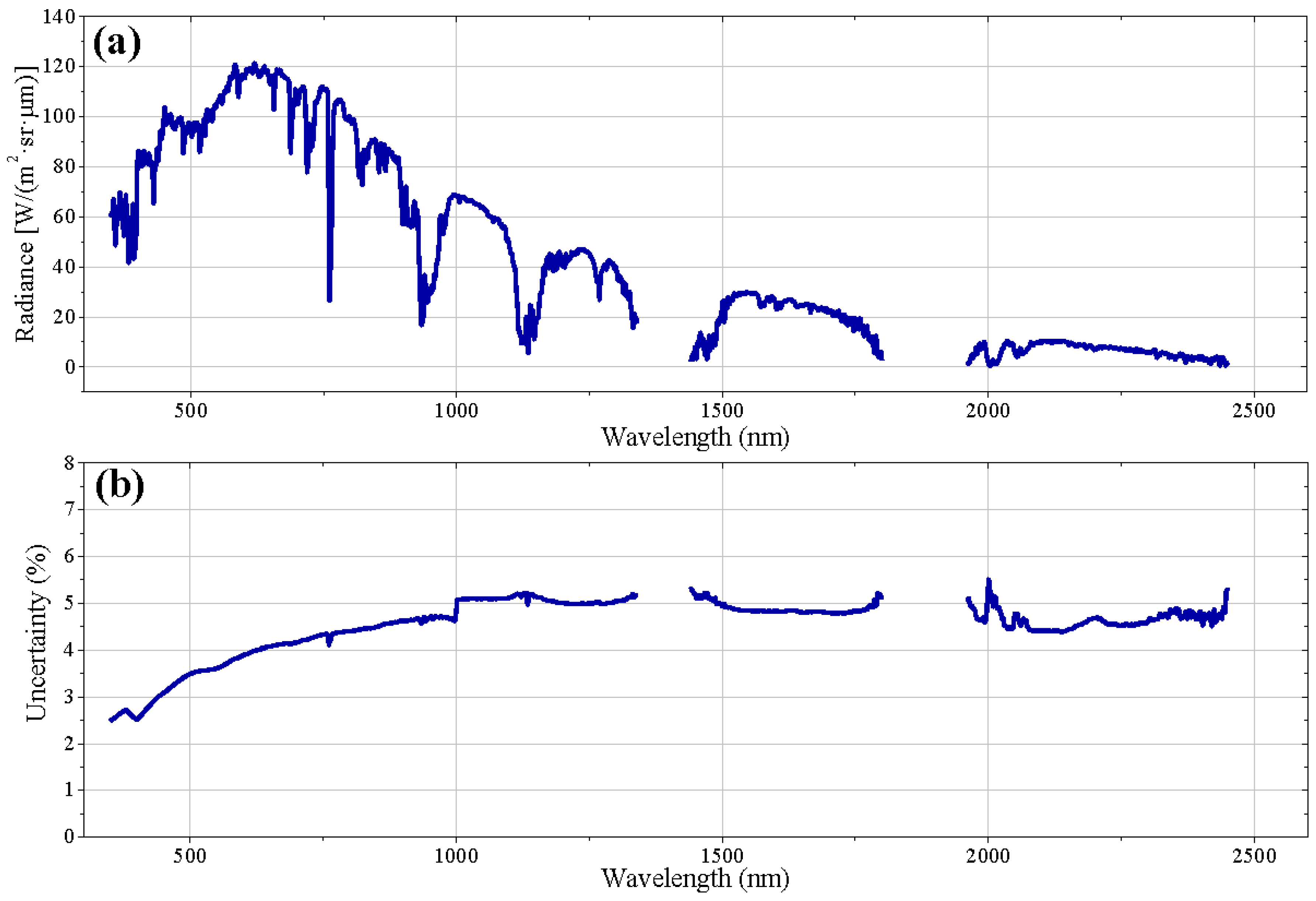
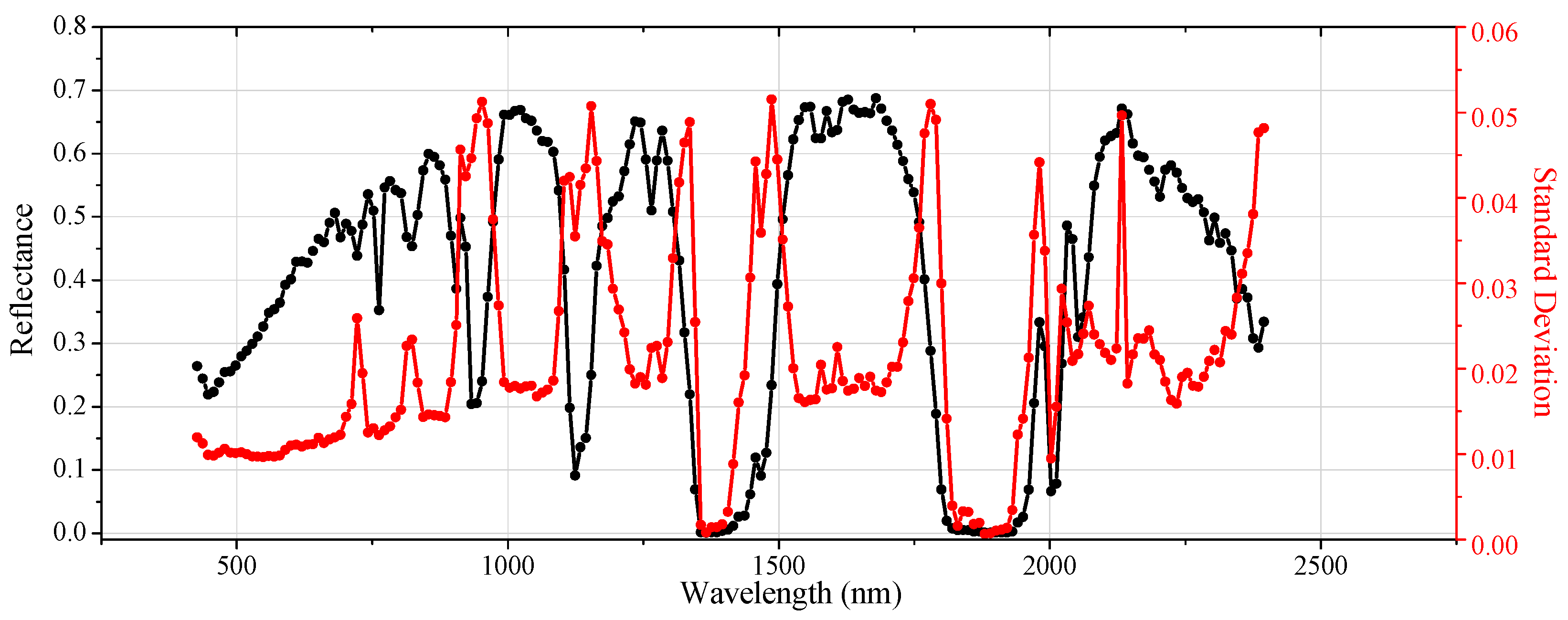
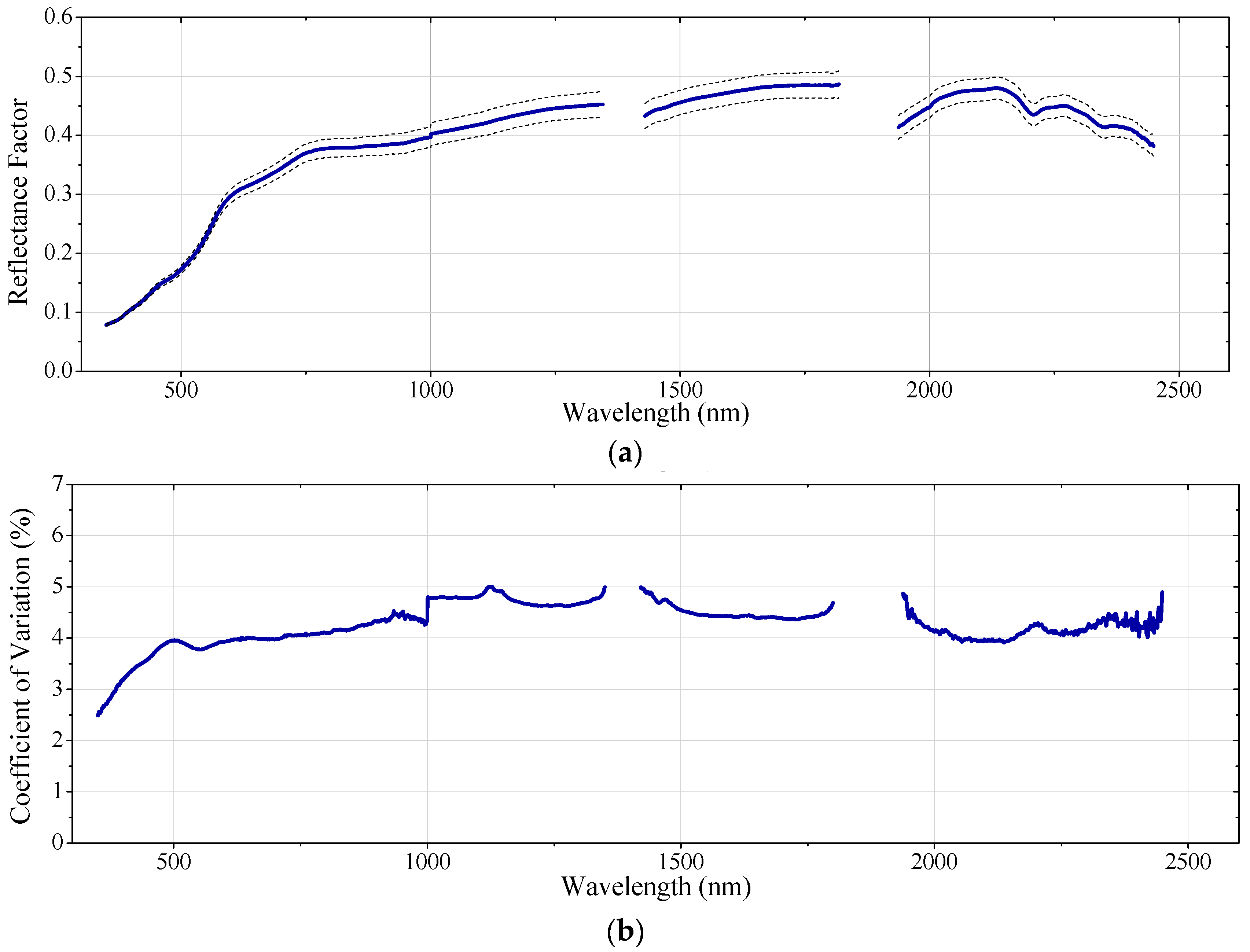
Figure 7a shows the spectral reflectance derived for the Algodones Dunes sand surface on 9 March 2015. In addition, the coefficient of variation (CV) defined as the ratio between the standard deviation and the average is shown as a percentage in Figure 7b. The gaps around 1400 and 1800 nm are due to strong water vapor absorption near those wavelengths and the 2400–2500 nm spectral region shows larger variability primarily due to decreasing signal level.
According to [43], reflectance values higher than 0.3 over the entire spectral range are preferred. The selected reference surface at Algodones Dunes presents reflectance higher than 0.3 in almost the entire spectral range. As seen in Figure 7a, the average reference surface reflectance factor was between 0.08 and 0.30 from 350–600 nm and between 0.30 and 0.49 from 600–2500 nm. Scott et al. (1996) [43] suggest that a certain surface is sufficiently spatially uniform if the Coefficient of Variation (CV) is lower than 5%. The average relative CV of the spectral measurements ranged from 2.5% to 5.0%, indicating that the reference surface at Algodones Dunes presents a spatial uniformity better than 5%.
The weather on 9 and 10 March 2015 was clear with no clouds. The atmosphere was stable during the entire period of measurement, from 9 a.m. to 12:30 p.m. (local time), as well as the time around CBERS-4 overpass. The atmospheric conditions for both dates are summarized in Table 5.
Aerosol optical depth (AOD) is a measure of radiation extinction due to the interaction of radiation with aerosol particles in the atmosphere. According to [27], the variation in AOD with wavelength defines the attenuation of solar irradiance as a function of wavelength and provides the basis for retrieving the columnar size distribution of the atmospheric aerosol. An AOD lower than 0.1 indicates clear sky, whereas value of 1 corresponds to very hazy conditions [44]. Here, the mean AOD at 550 nm was 0.066 ± 0.017 and 0.046 ± 0.014 during the measurements on 9 and 10 March 2015, respectively, indicating that the Algodones Dunes region presents low aerosol loading.
Columnar water vapor was derived from the solar extinction data using a modified Langley approach. The water content was (1.055 ± 0.014) g/cm2 on 9 March 2015 and (0.476 ± 0.005) g/cm2 on 10 March 2015.
The surface reflectance, geometric and atmospheric conditions were used as inputs to MODTRAN. Figure 8 gives the at-sensor radiance (TOA radiance) predicted by MODTRAN. Table 6 presents the band-averaged TOA radiance (using Equation (4)) for each of the four multispectral bands of MUX and WFI derived from the spectral curve in Figure 1. Table 6 also presents the average DN from the image for each band based on the 8 × 15 grid (120 pixels) for MUX and based on the 2 × 5 grid (10 pixels) for WFI.
Past work with the reflectance-based method as used here indicated that the method presented absolute uncertainties of ±5%, and estimated that improvements should result in an uncertainty of ±3% in the middle of the visible portion of the spectrum [21]. In this work, as can been seen in Table 6, the uncertainty in the TOA Radiance predicted by MODTRAN ranged from 3.1% to 4.4% in the four MUX and WFI spectral bands. There are several sources of uncertainty in this method: (i) surface characterization; (ii) atmospheric characterization; (iii) radiative transfer code; (iv) determination of the site-average DNs. Here, the main source of uncertainty was the reflectance surface (about 2.5%–5.0%), which supports the importance of properly choosing a reference surface for calibration.
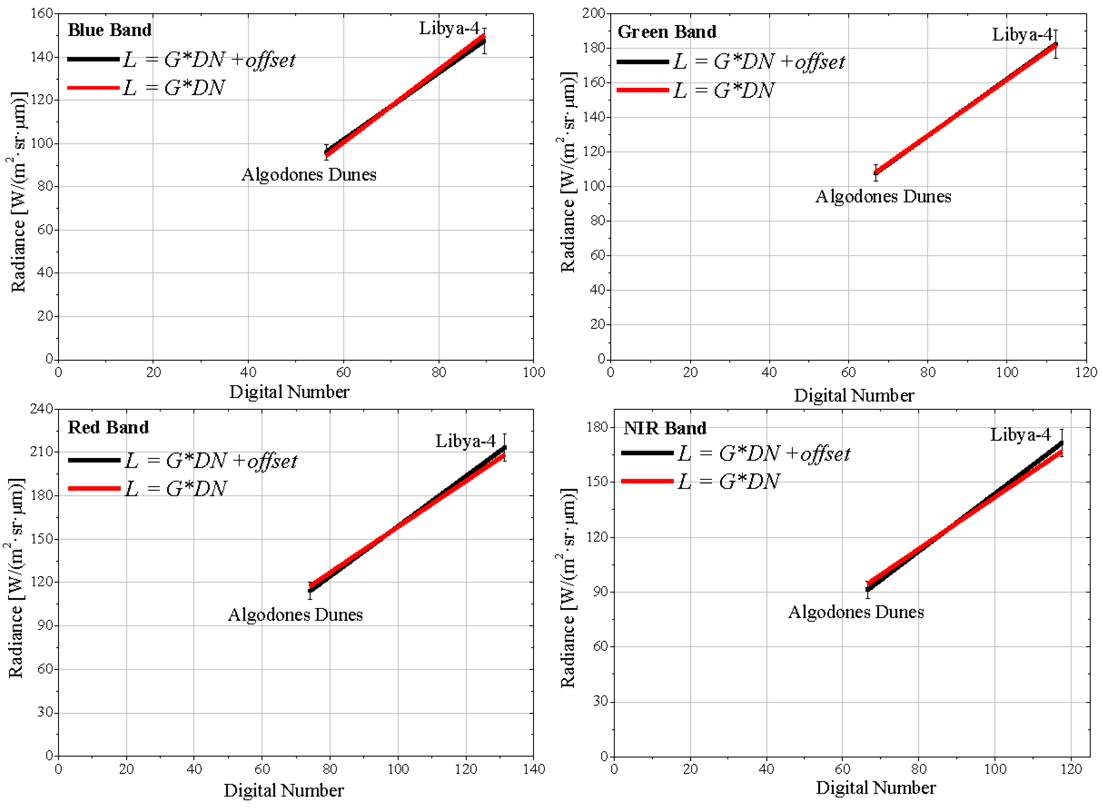
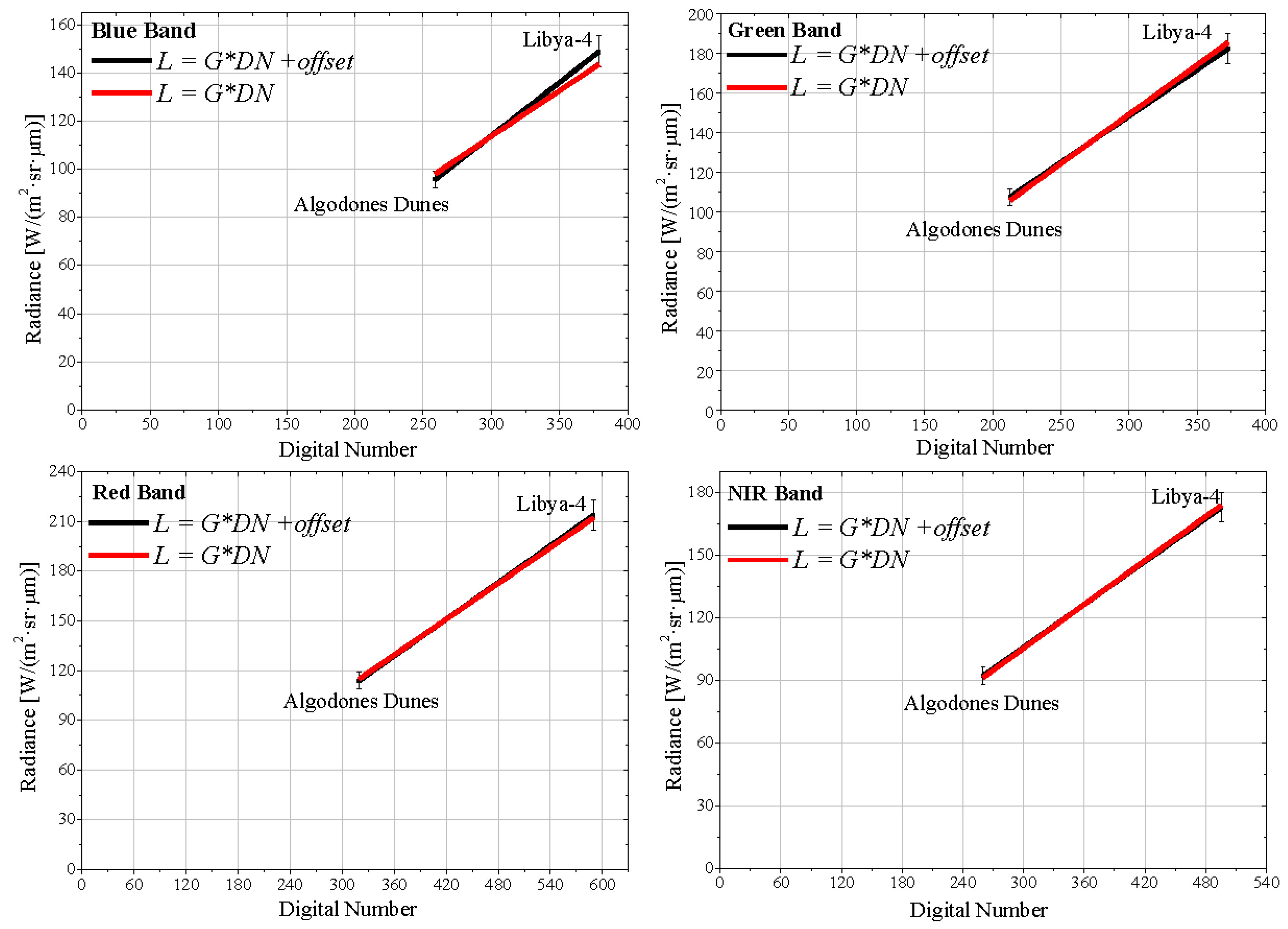
To determine the two radiometric calibration coefficients, Gi and offseti, for MUX and WFI, two points were considered. With the reflectance-based method it was possible to obtain one point (see Table 6) and through cross-calibration another point was generated. The cross-calibration results between CBERS-4 and Landsat-8 using images acquired from Libya-4 can be seen in Table 7. In order to convert the values in Landsat-8/OLI image to TOA reflectance the methodology presented in [45] was used. The radiance values of the MUX and WFI sensors, Lλ,MUX and Lλ,WFI, were estimated using Equation (8), i.e., the radiance values were obtained from the OLI sensor radiance, Lλ,OLI.
The calibration gains for the MUX and WFI sensors are computed by linearly regressing their predicted at-sensor radiances against the measured raw counts. The measurements over Algodones Dunes and from the Libya-4 PICS are used together during regression to achieve a greater dynamic range. The regression slope provides the radiometric gain of the sensor. The linear fits were implemented using the Method of Least Squares [46]. Using the ISO-GUM method (called also “Law of propagation of uncertainty”, see Section 6) was possible to estimate the uncertainties of the coefficients slope or intercept [46]. Two sets of calibration slopes are computed: one using the standard linear fit with an offset term, and second without an offset term, where the linear regression is forced through origin. The two sets of regression plots for the CBERS-4 MUX and WFI bands are shown in Figure 9 and Figure 10, respectively. The calibration coefficients derived from these linear regressions are listed in Table 8.
Taking into account the uncertainties, all the intercept coefficients (with free intercept) are consistent with zero, indicating that the offseti from Equation (1) is zero, i.e., there was no statistical evidence for using offsets other than zero for all spectral bands on both sensors. This result was expected, since when there is no incident energy on the sensor aperture the expected response is zero. Regarding the gain coefficients, the uncertainties ranged from 8.8%–13.6%. It is important to note that in this fit, with free intercepts, the degree of freedom is zero.
The zero-intercept linear fits yield very good coefficients of determination, ranging from 0.98 to 1.00, in all four spectral bands of MUX and WFI. The slopes (gain coefficient) were determined with uncertainties within 2.8%–3.5% for both MUX and WFI sensors.
As mentioned earlier, a calibration coefficient validation was performed using cross-calibration techniques. A comparison was done between Landsat-7 ETM+ and at-sensor reflectance derived from MUX and WFI measurements. To convert the values in the Landsat-7 image to TOA reflectance the methodology presented in [7] was used. To determine TOA reflectance from MUX and WFI images, Equation (2) was used. The spectral radiance at the sensor’s aperture was estimated by applying Equation (1), where the calibration coefficients, Gi and offseti, are shown in Table 8. The solar exoatmospheric spectral irradiances for MUX and WFI bands are summarized in Table 2. 
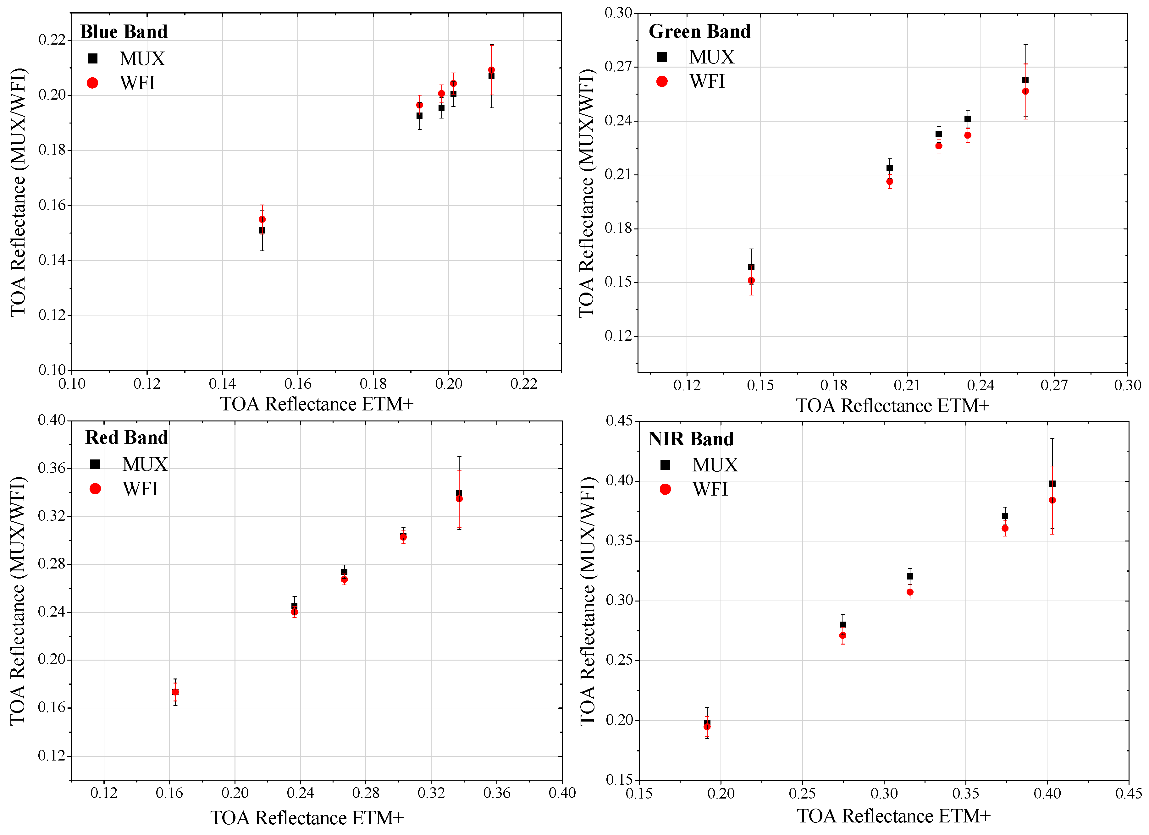
Figure 11 shows a graphic of ETM+ TOA reflectance as a function of MUX and WFI TOA reflectance values for the five ROIs using the Gi with zero-intercept linear fits.
It is clearly possible to verify in Figure 11 that the relationship between Landsat-7 (ETM+) TOA reflectance and CBERS-4 (MUX and WFI) TOA reflectance is linear, supporting the idea that the detector response is linear. Furthermore, the reflectance values of the three sensors (ETM+, MUX and WFI) are compatible within the associated uncertainty with each of them.
Table 9 provides the percentage differences in TOA reflectance of the five ROIs between MUX/WFI and ETM+ similar bands after applied the spectral band adjustment. A negative sign in the difference indicates that the value measured by the ETM+ sensor band is higher than the corresponding CBERS-4 sensors bands. On average the absolute difference between CBERS-4 (MUX and WFI) and Landsat-7/EMT+ in the analogous bands was 3.3% and 2.2% when it was used the calibration coefficients determined with free intercept and when forced zero intercept, respectively. This result reinforces the idea that the coefficient offseti from Equation (1) is zero (as mentioned earlier), since the difference between CBERS-4 and Landsat-7 is lower when it uses only the gain coefficient (forced zero intercept).
A convenient way to assess the consistency of these results is to compare them with the calibration uncertainties estimated. The uncertainties in the gain coefficients for zero-intercept linear fits ranged from 2.8% to 3.4%; therefore, the associated uncertainties cover the differences. Thus, in all of the four MUX and WFI spectral bands, these results are well within the specified calibration uncertainties. Remembering that the uncertainties values were quoted with a confidence level of 68.3% (as one-sigma percentages).

8. Conclusions

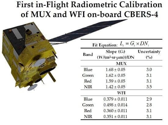
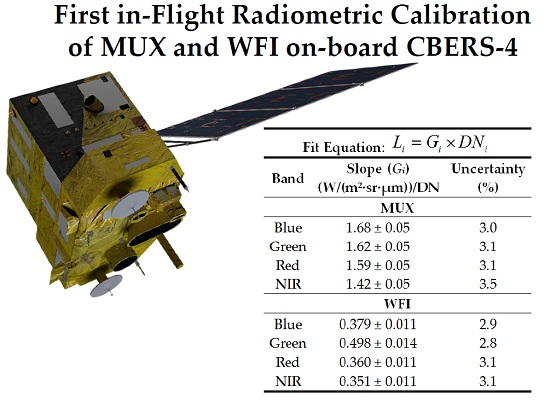
Brazil and China have a long-term joint space program: the China-Brazil Earth Resources Satellite (CBERS). The last satellite of this program (CBERS-4) was launched on 7 December 2014. The extraction of quantitative information from data collected by sensors on-board CBERS-4 is only possible through a well-performed absolute calibration. This work describes the complete procedure to calculate the in-flight absolute calibration coefficients for sensor MUX and WFI (CBERS-4) images.
The reflectance-based approach and cross-calibration method were applied. An area at the Algodones Dunes region located in southwestern USA was used as a reference surface for the reflectance-based approach. The cross-calibration between both MUX and WFI on-board CBERS-4 and the Operational Land Imager (OLI) on-board Landsat-8 was performed using Libya-4 Pseudo Invariant Calibration Site.
There was no statistical evidence for using offsets other than zero for all bands on both sensors. The gain coefficients are now available for data users: 1.68, 1.62, 1.59 and 1.42 for MUX sensor and 0.379, 0.498, 0.360 and 0.351 for WFI spectral bands blue, green, red and NIR, respectively, in units of (W/(m2·sr·μm))/DN. These coefficients were determined with uncertainties within 2.8%–3.5%. It is noteworthy that this current work is the first one to present the uncertainty in the CBERS series calibration. Thus, the results achieved here are considered as important progress in the calibration of the Brazilian and Chinese satellite.
A procedure to validate the estimated coefficients was performed using cross-calibration techniques. The results were presented as percentage of disagreement between the Landsat-7 EMT+ and at-sensor reflectance reported using the above mentioned coefficients calibration of MUX and WFI. On average, the difference was 2.2% (after application of the spectral band adjustment), indicating good agreement with the well accepted Landsat 7 ETM+ results.
It is important to emphasize the need to preserve the accuracy of the MUX and WFI absolute radiometric calibration by recalibration on-orbit regularly. It is necessary to perform evaluations of the sensor radiometric once on-orbit, as well as during its operational life, to ensure the on-orbit radiometric stability of the instruments.

Acknowledgments

The authors would like to thank to the Conselho Nacional de Desenvolvimento Científico e Tecnológico (CNPq) and the Coordenação de Aperfeiçoamento de Pessoal de Nível Superior (CAPES) for the scholarship given to Cibele T. Pinto and the research financial support.

Author Contributions

Cibele Pinto was responsible for the data analysis, main research ideas and writing the manuscript. Larry Leigh was involved in the data collection at Algodones Dunes campaign and provided expertise to process MODTRAN. David Aaron performed the major edits of this manuscript. Flávio Ponzoni, Ruy Castro, Nischal Mishra and Dennis Helder contributed to the research ideas, provided valuable data analysis and insights into the organization of the various sections of the paper. All authors thoroughly reviewed and edited this paper.

Conflicts of Interest

The authors declare no conflict of interest.

References

  1. Ponzoni, F.J.; Zullo, J., Jr.; Lamparelli, R.A.C. In-flight absolute calibration of the CBERS-2 CCD sensor data. Ann. Braz. Acad. Sci. 2008, 80, 373–380. [Google Scholar] [CrossRef]
  2. Epiphanio, J.C.N. CBERS: Estado atual e future. In Proceedings of the Brazilian Remote Sensing Symposium, Natal, Brazil, 25–30 April 2009; pp. 2001–2008.
  3. Epiphanio, J.C.N. CBERS-3/4: Características e potencialidades. In Proceedings of the Brazilian Remote Sensing Symposium, Curitiba, Brazil, 30 April–5 May 2011; pp. 9009–9016.
  4. Thome, K.J.; Helder, D.L.; Aaron, D.; Dewald, J.D. Landsat-5 TM and Landsat-7 ETM+ absolute radiometric calibration using the reflectance-based method. IEEE Trans. Geosci. Remote Sens. 2004, 42, 2777–2785. [Google Scholar] [CrossRef]
  5. Thome, K.J.; Markham, B.L.; Barker, J.L.; Slater, P.N.; Biggar, S.F. Radiometric calibration of Landsat. Photogramm Eng. Rem. Sens. 1997, 63, 853–858. [Google Scholar]
  6. Helder, D.L.; Markham, B.L.; Thome, K.J.; Barsi, J.A.; Chander, G.; Malla, R. Updated radiometric calibration for the Landsat-5 thematic mapper reflective bands. IEEE Trans. Geosci. Remote Sens. 2008, 46, 3309–3325. [Google Scholar] [CrossRef]
  7. Chander, G.; Markham, B.L.; Helder, D.L. Summary of current radiometric calibration coefficients for Landsat MSS, TM, ETM+, and EO-1 ALI sensors. Remote Sens. Environ. 2009, 113, 893–903. [Google Scholar] [CrossRef]
  8. Markham, B.L.; Haque, M.D.O.; Barsi, J.A.; Micijevic, E.; Helder, D.L.; Thome, K.J.; Aaron, D.; Czapla-myers, J.S. Landsat-7 ETM+: 12 Years on-orbit reflective-band radiometric performance. IEEE Trans. Geosci. Remote Sens. 2012, 50, 2056–2062. [Google Scholar] [CrossRef]
  9. Slater, P.N.; Biggar, S.F.; Holm, R.G.; Jackson, R.D.; Mao, Y.; Moran, M.S.; Palmer, J.M.; Yuan, B. Reflectance-and radiance-based methods for the in-flight absolute calibration of multispectral sensors. Remote Sens. Environ. 1987, 22, 11–37. [Google Scholar] [CrossRef]
  10. Thome, K.J. Absolute radiometric calibration of Landsat-7 ETM+ using the reflectance-based method. Remote Sens. Environ. 2001, 78, 27–38. [Google Scholar] [CrossRef]
  11. Ponzoni, F.J.; Zullo, J.J.R.; Lamparelli, R.A.C.; Pellegrino, G.Q.; Arnaud, Y. In-flight absolute calibration of the Landsat 5 TM on the test site salar de Uyuni. IEEE Trans. Geosci. Remote Sens. 2004, 42, 2761–2766. [Google Scholar] [CrossRef]
  12. Teillet, P.M.; Markham, B.L.; Irish, R.R. Landsat cross-calibration based on near simultaneous imaging of common ground targets. Remote Sens. Environ. 2006, 102, 264–270. [Google Scholar] [CrossRef]
  13. Helder, D.L.; Bikash, B.; DanieL, L.M. Optimized identification of worldwide radiometric pseudo-invariant calibration sites. Can. J. Remote Sens. 2010, 36, 527–539. [Google Scholar] [CrossRef]
  14. Helder, D.L.; Thome, K.J.; Mishra, N.; Chander, G.; Xiong, X.; Angal, A.; Choi, T. Absolute radiometric calibration of Landsat using a pseudo invariant calibration site. IEEE Trans. Geosci. Remote Sens. 2013, 51, 1360–1369. [Google Scholar] [CrossRef]
  15. Mishra, N.; Helder, D.L.; Angal, A.; Choi, J.; Xiong, X. Absolute calibration of optical satellite sensors using Libya 4 pseudo invariant calibration site. Remote Sens. 2014, 6, 1327–1346. [Google Scholar] [CrossRef]
  16. Cosnefroy, H.; Leroy, M.; Briottet, X. Selection of Sahara and Arabien desert sites for calibration of optical satellite sensors. Remote Sens. Environ. 1996, 58, 101–114. [Google Scholar] [CrossRef]
  17. Pinto, C.T.; Ponzoni, F.J.; Castro, R.M.; Griffith, D.J. Spectral uniformity evaluation of reference surfaces for airborne and orbital sensors absolute calibration. Braz. J. Geophys. 2012, 30, 263–275. [Google Scholar]
  18. Nicodemus, F.E.; Richmond, J.C.; Hsia, J.J.; Ginsberg, I.W.; Limperis, T. Geometrical Considerations and Nomenclature for Reflectance. National Bureau of Standards, United States department of Commerce, 1977. Available online: https://graphics.stanford.edu/courses/cs448–05-winter/papers/nicodemus-brdf-nist.pdf (accessed on 20 January 2016).
  19. Schaepman-strub, G.; Schapman, M.E.; Painter, T.H.; Dangel, S.; Martonchik, J.V. Reflectance quantities in optical remote sensing—Definitions and case studies. Remote Sens. Environ. 2006, 103, 27–42. [Google Scholar] [CrossRef]
  20. Milton, E.J. Principles of field spectroscopy. Int. J. Remote Sens. 1987, 8, 1807–1827. [Google Scholar] [CrossRef]
  21. Czapla-Myers, J.; McCorkel, J.; Anderson, N.; Thome, K.; Biggar, S.; Helder, D.; Aaron, D.; Leigh, L.; Mishra, N. The ground-based absolute radiometric calibration of Landsat 8 OLI. Remote Sens. 2015, 7, 600–626. [Google Scholar] [CrossRef]
  22. Hatchell, D.C. Analytical Spectral Devices Technical Guide, 3rd ed.; Analytical Spectral Devices: Boulder, CO, USA, 1999. [Google Scholar]
  23. Labsphere Inc. Setting the Standard in Light Measurement: Product Guide; Labsphere: Sutton, NH, USA, 2009. [Google Scholar]
  24. Helder, D.L.; Thome, K.; Aaron, D.; Leigh, L.; Czapla-Myers, J.; Leisso, N.; Biggar, S.; Anderson, N. Recent surface reflectance measurement campaigns with emphasis on best practices, SI traceability and uncertainty estimation. Metrologia 2012, 49, S21–S28. [Google Scholar] [CrossRef]
  25. Ehsani, A.R.; Reagan, J.A.; Erxleben, W.H. Design and performance analysis of an automated 10-channel solar radiometer instrument. J. Atmos. Ocean. Technol. 1998, 15, 697–707. [Google Scholar] [CrossRef]
  26. Schmid, B.; Wehrli, C. Comparison of sun photometer calibration by use of the Langley technique and the standard lamps. Appl. Opt. 1995, 34, 4500–4512. [Google Scholar] [CrossRef] [PubMed]
  27. Rollin, E.M. An introduction to the use of Sun-photometry for the atmospheric correction of airborne sensor data. Activities of the NERC EPFS in support of the NERC ARSF. In Proceedings of the ARSF Annual Meeting, Keyworth, UK, 2000.
  28. Pinto, C.T.; Ponzoni, F.J.; Barrientos, C.; Mattar, C.; Santamaría-Artigas, A.; Castro, R.M. Spectral and atmospheric characterization of a site at Atacama Desert for earth observation sensors calibration. IEEE Geosci. Remote Sens. Lett. 2015, 12, 2227–2231. [Google Scholar] [CrossRef]
  29. Ponzoni, F.J.; Pinto, C.T.; Lamparelli, R.A.C.; Zullo, J., Jr.; Antunes, M.A.H. Calibração de Sensores Orbitais, 2nd ed.; Oficina de Textos: São José dos Campos, Brazil, 2015. [Google Scholar]
  30. Halthore, R.N.; Eck, T.F.; Holben, B.N.; Markham, B.L. Sun photometric measurements of atmospheric water vapor column abundance in the 940-nm band. J. Geophys. Res. Atmos. 1997, 102, 4343–4352. [Google Scholar] [CrossRef]
  31. Berk, A.; Anderson, G.P.; Acharya, P.K.; Shettle, E.P. MODTRAN 5.2.1 User’s Manual; Spectral Sciences Inc.: Burlington, MA, USA; Air Force Research Laboratory: Hanscom AFB, MA, USA, 2011. [Google Scholar]
  32. Ientilucci, E.J. Using MODTRAN Predicting Sensor-Reaching Radiance; Chester, F. Carlson Center for Imaging Science and Rochester Institute of Technology: Rochester, NY, USA, 2007. [Google Scholar]
  33. Irons, J.R.; Dwyer, J.L.; Barsi, J.A. The next Landsat satellite: The Landsat data continuity mission. Remote Sens. Environ. 2012, 122, 11–21. [Google Scholar] [CrossRef]
  34. Teillet, P.M.; Barker, J.L.; Markham, B.L.; Irish, R.R.; Fedosejevs, G.; Storey, J.C. Radiometric cross-calibration of the Landsat-7 ETM+ and Landsat-5 TM sensors based on tandem data sets. Remote Sens. Environ. 2001, 78, 39–54. [Google Scholar] [CrossRef]
  35. Chander, G.; Mishra, N.; Helder, D.L.; Aaron, D.B.; Angal, A.; Choi, T.; Xiong, X.; Doelling, D.R. Applications of spectral band adjustment factors (SBAF) for cross-calibration. IEEE Trans. Geosci. Remote Sens. 2013, 51, 1267–1281. [Google Scholar] [CrossRef]
  36. Henry, P.; Chander, G.; Fougnie, B.; Thomas, C.; Xiong, X. Assessment of spectral band impact on intercalibration over dessert sites using simulation based on EO-1 Hyperion data. IEEE Trans. Geosci. Remote Sens. 2013, 51, 1297–1308. [Google Scholar] [CrossRef]
  37. Markham, B.; Thome, K.J.; Barsi, J.A.; Kaita, E.; Helder, D.L.; Barker, J.L.; Scaramuzza, P.L. Landsat-7 ETM+ on-orbit reflective-band radiometric stability and absolute calibration. IEEE Trans. Geosci. Remote Sens. 2004, 42, 2810–2820. [Google Scholar] [CrossRef]
  38. Joint Committee for Guides in Metrology and Bureau International des Poids et Mesures. Evaluation of Measurement Data—Guide to the Expression of Uncertainty in Measurement, 1st ed.; JCGM: Pavillon de Breteuil, France, 2008. [Google Scholar]
  39. Joint Committee for Guides in Metrology and Bureau International des Poids et Mesures. Evaluation of Measurement Data—Supplement 1 to the “Guide to the Expression of Uncertainty in measurement”—Propagation of Distributions Using a Monte Carlo Method, 1st ed.; JCGM: Pavillon de Breteuil, France, 2008. [Google Scholar]
  40. Chen, W.; Zhao, H.; Li, Z.; Jing, X.; Yan, L. Uncertainty evaluation of an in-flight absolute radiometric calibration using a statistical Monte Carlo method. IEEE Trans. Geosci. Remote Sens. 2015, 53, 2925–2934. [Google Scholar] [CrossRef]
  41. Pinto, C.T.; Ponzoni, F.J.; Fonseca, L.M.G.; Castro, R.M. Simulação de Monte Carlo na avaliação das incertezas em parte do processo de calibração de sensores. In Proceedings of the Brazilian Remote Sensing Symposium, Foz do Iguaçu, Brazil, 13–18 April 2013; pp. 9131–9137.
  42. Biggar, S.F.; Slater, P.N.; Gellman, D.I. Uncertainties in the in-flight calibration of sensors with reference to measured ground sites in the 0.4–1.1 µm range. Remote Sens. Environ. 1994, 48, 245–252. [Google Scholar] [CrossRef]
  43. Scott, K.P.; Thome, K.J.; Bronwlee, M.R. Evaluation of the Railroad Valley Playa for use in vicarious calibration. Proc. SPIE 1996, 2818, 158–166. [Google Scholar]
  44. Gro, S.; Esselborn, M.; Wirth, M.; Fix, A.; Minikin, A. Airborne high spectral resolution lidar observation of pollution aerosol during EUCAARI-LONGREX. Atmos. Chem. Phys. 2013, 13, 2435–2444. [Google Scholar] [Green Version]
  45. Mishra, N.; Haque, M.O.; Leigh, L.; Aaron, D.; Helder, D.; Markham, B. Radiometric cross calibration of Landsat 8 Operational Land Imager (OLI) and Landsat 7 Enhanced Thematic Mapper Plus (ETM+). Remote Sens. 2014, 6, 12619–12638. [Google Scholar] [CrossRef]
  46. Bevington, P.R.; Robinson, D.K. Data Reduction and Error Analysis: For the Physical Sciences, 3rd ed.; McGraw-Hill Higher Education: New York, NY, USA, 2003. [Google Scholar]
Figure 1. Multispectral Camera (MUX), Wide-Field Imager (WFI), Operational Land Imager (OLI) and Enhanced Thematic Mapper Plus (ETM+) Spectral Response Function (SRF).
Remotesensing 08 00405 g001
Figure 2. (a) Algodones Dunes location; and (b) MUX/CBERS-4 image from study area. The red box indicates the location of the field campaign surface.
Remotesensing 08 00405 g002
Figure 3. Spectralon panel measurements collection.
Remotesensing 08 00405 g003
Figure 4. Libya-4 image from (a) Landsat-8/OLI (b) CBERS-4/MUX and (c) CBERS-4/WFI. The red box indicates the location of the study area.
Remotesensing 08 00405 g004
Figure 5. Average TOA reflectance profile of 224 EO-1 Hyperion images over Libya-4 from 2004 to 2014.
Remotesensing 08 00405 g005
Figure 6. Algodones Dunes image from (a) EO-1/Hyperion; (b) Landsat-7/EMT+; (c) CBERS-4/MUX and (d) CBERS-4/WFI. The five red boxes indicate the location of the five ROIs.
Remotesensing 08 00405 g006
Figure 7. (a) Spectral reflectance results of 160 × 300 m site at Algodones Dunes on 9 March 2015. The solid line shows the average reflectance and the dashed line shows the maximum and minimum variation of the average (±1σ); (b) Surface Coefficient of Variation in percentage.
Remotesensing 08 00405 g007
Figure 8. (a) Top of Atmosphere radiance predicted by MODTRAN and (b) relative uncertainty.
Remotesensing 08 00405 g008
Figure 9. Absolute radiometric calibration of MUX/CBERS-4.
Remotesensing 08 00405 g009
Figure 10. Absolute radiometric calibration of WFI/CBERS-4.
Remotesensing 08 00405 g010
Figure 11. TOA reflectance comparison between Landsat-7 ETM+ and CBERS-4 (MUX and WFI) after application of the SBAF.
Remotesensing 08 00405 g011
Table 1. Summary of the MUX and WFI on-board CBERS-4 characteristics.
CharacteristicMUXWFI
TechniquePushbroomPushbroom
Altitude778 km778 km
Swath Width120 km866 km
Field of View (FOV)±4°±28.63°
Spectral Bands (nm)450–520 (Blue)450–520 (Blue)
520–590 (Green)520–590 (Green)
630–690 (Red)630–690 (Red)
770–890 (NIR)770–890 (NIR)
Spatial Resolution20 m64 m (nadir)
Temporal Resolution26 days5 days
Radiometric Resolution8 bits10 bits
Source: Epiphanio (2003) [3].
Table 2. Solar Exoatmospheric spectral irradiances (ESUNλ) for MUX and WFI spectral bands.
Spectral Bands (nm)ESUNλ MUX (W/(m2·μm))ESUNλ WFI (W/(m2·μm))
450–520 (Blue)1958 ± 351952 ± 35
520–590 (Green)1852 ± 291852 ± 29
630–690 (Red)1559 ± 181545 ± 18
770–890 (NIR)1091 ± 111098 ± 11
Table 3. Metadata of scenes used for MUX, WFI/OLI cross-calibration.
Satellite/SensorDateAcquisition Time (UTC)Path/RowSolar Zenith AngleSolar Azimuth AngleLook Angle
Landsat 8/OLI11 July 201508:54181/04022.5°102.0°Nadir
CBERS-4/MUX7 July 201509:20095/06817.2°106.6°Nadir
CBERS-4/WFI7 July 201509:20094/06916.4°106.3°Nadir
Table 4. Metadata of scenes used for MUX, WFI/ETM+ cross validation.
Satellite/SensorDateAcquisition Time (UTC)Path/RowSolar Zenith AngleSolar Azimuth AngleLook Angle
Landsat 7/ETM+10 March 201518:15:2839/3743.7°143.5°Nadir
CBERS-4/MUX9 March 201518:33:29238/6342.1°151.9°Nadir
CBERS-4/WFI9 March 201518:33:29238/6342.1°151.9°Nadir
EO-1/Hyperion9 March 201517:10:4039/3753.6°126.3°18.1°
Table 5. Summary of atmospheric conditions.
9 March 2015
Julian Day68
Local Time9:00–12:30
Aerosol Optical Depth at 550 nm (dimensionless)0.066 ± 0.017
Water vapor (g/cm2)1.055 ± 0.014
VIS (km)40.4 ± 2.3
Temperature (°C)23 ± 4
Pressure (hPa)999.64 ± 0.13
10 March 2015
Julian Day69
Local Time9:00–12:30
Aerosol Optical Depth at 550 nm (dimensionless)0.046 ± 0.014
Water vapor (g/cm2)0.476 ± 0.005
VIS (km)48.0 ± 2.6
Temperature (°C)26 ± 3
Pressure (hPa)999.26 ± 0.26
Table 6. Summary of reflectance-based approach results using Algodones Dunes site of 160 by 300.
BandTOA Radiance Predicted by MODTRAN (W/(m2·sr·μm))Uncertainty (%)Digital NumberUncertainty (%)TOA Radiance Predicted by MODTRAN (W/(m2·sr·μm))Uncertainty (%)Digital NumberUncertainty (%)
MUXWFI
Blue96 ± 33.156.3 ± 1.12.096 ± 33.1258.8 ± 2.71.0
Green108 ± 43.766.8 ± 1.62.4108 ± 43.7212.7 ± 2.91.4
Red114 ± 54.474.2 ± 1.92.6114 ± 54.4320 ± 51.6
NIR91 ± 44.466.6 ± 1.62.493 ± 44.3260 ± 31.2
Table 7. Landsat-8/OLI and CBERS-4 (MUX and WFI) cross-calibration results using Libya-4 site.
BandTOA Radiance from OLI (after Corrections) (W/(m2·sr·μm))Uncertainty (%)Digital NumberUncertainty (%)TOA Radiance from OLI (after Corrections) (W/(m2·sr·μm))Uncertainty (%)Digital NumberUncertainty (%)
MUXWFI
Blue147 ± 42.790 ± 33.3149 ± 42.7379 ± 123.2
Green183 ± 52.7112 ± 43.6182 ± 52.7373 ± 123.2
Red214 ± 62.8131 ± 43.1214 ± 62.8590 ± 172.9
NIR171 ± 52.9118 ± 43.4173 ± 52.9495 ± 132.6
Table 8. Linear fits results corresponding to the plots shown in Figure 9 and Figure 10.
Fit Equation: L i = G i × D N i + o f f s e t i (Free Intercept)Fit Equation: L i = G i × D N i (Forced Zero Intercept)
BandSlope (Gi) (W/(m2·sr·μm))/DNUncertainty (%)Intercept (offseti) (W/(m2·sr·μm))Uncertainty (%)Slope (Gi) (W/(m2·sr·μm))/DNUncertainty (%)
MUX
Blue1.54 ± 0.2113.69 ± 141561.68 ± 0.053.0
Green1.64 ± 0.2112.8−2 ± 178501.62 ± 0.053.1
Red1.73 ± 0.1911.0−14 ± 181291.59 ± 0.053.1
NIR1.57 ± 0.1811.5−13 ± 151151.42 ± 0.053.5
WFI
Blue0.44 ± 0.0613.6−19 ± 18950.379 ± 0.0112.9
Green0.47 ± 0.0510.68 ± 141750.498 ± 0.0142.8
Red0.37 ± 0.0410.8−4 ± 153750.360 ± 0.0113.1
NIR0.34 ± 0.038.83 ± 124000.351 ± 0.0113.1
Table 9. Landsat-7 and CBERS-4 percentage difference in TOA reflectance of the five ROIs.
BandDiff after SBAF ETM+/MUXDiff after SBAF ETM+/WFIDiff after SBAF ETM+/MUXDiff after SBAF ETM+/WFI
L i = G i × D N i + o f f s e t i L i = G i × D N i
ROI 1
Blue4.62%−7.25%0.27%2.93%
Green6.77%9.87%8.52%3.34%
Red−7.82%2.30%5.78%5.92%
NIR−11.95%4.59%3.40%1.76%
ROI 2
Blue1.64%−2.07%0.12%2.17%
Green4.41%4.95%5.34%1.74%
Red−3.09%−0.10%3.67%1.62%
NIR−5.71%0.25%1.94%−1.38%
ROI 3
Blue−1.41%−3.63%−2.09%−1.05%
Green1.18%0.77%1.68%−0.70%
Red−1.56%−1.12%0.71%−0.69%
NIR−3.37%−4.83%−1.27%−4.72%
ROI 4
Blue0.67%−1.82%−0.40%1.49%
Green3.60%3.86%4.34%1.43%
Red−2.44%−1.02%2.61%0.22%
NIR−3.89%−2.12%1.41%−2.75%
ROI 5
Blue−0.11%−2.30%−1.36%1.24%
Green2.09%1.07%2.76%−1.14%
Red−3.23%−0.81%0.34%−0.04%
NIR−4.00%−3.59%−0.94%−3.67%

