Advancements for Snowmelt Monitoring by Means of Sentinel-1 SAR

Abstract

The Sentinel satellite constellation series, developed and operated by the European Space Agency, represents the dedicated space component of the European Copernicus program, committed to long-term operational services in environment, climate and security. We developed, tested and evaluated an algorithm for generating maps of snowmelt area from C-band synthetic aperture radar (SAR) data of the Sentinel-1 mission. For snowmelt classification, a change detection method is applied, using multitemporal dual-polarized SAR data acquired in Interferometric Wide swath (IW) mode, the basic operation mode over land surfaces. Of particular benefit for wet snow retrievals are the high instrument stability, the high spatial resolution across the 250 km wide swath, and the short revisit time. In order to study the impact of polarization, we generated maps of melting snow using data of the VV-polarized channel, the VH-polarized channel and a combined VV- and VH-based channel using a weighting function that accounts for effects of the local incidence angle. Comparisons are performed with snow maps derived from Landsat images over study areas in the Alps and in Iceland. The pixel-by-pixel comparisons show good agreement between the snow products of the two sensors, with the best performance for retrievals based on the combined (VV and VH) channel and a minor decline for the VH-based product. The VV-based snowmelt extent product shows a drop-off in quality over areas with steep terrain because of the decreasing backscatter contrast of snow-covered versus snow-free surfaces on fore-slopes. The investigations demonstrate the excellent capability of the Sentinel-1 mission for operational monitoring of snowmelt areas.

1. Introduction

The Sentinel satellite constellation series represents the dedicated space component of the European Earth observation program Copernicus, previously known as GMES (Global Monitoring for Environment and Security) [1]. Copernicus, coordinated and managed by the European Commission, provides global, timely and easily accessible information and services in application domains such as land, marine, atmosphere, emergency management, climate change and security [2]. In the final deployment stage, each of the six Sentinel missions that were developed and operated by the European Space Agency (ESA), comprises two satellites in order to fulfill the revisit and coverage requirements for a wide range of operational applications.

Sentinel-1A, the first dedicated satellite of the Copernicus program, was launched on 3 April 2014. The Sentinel-1 (S1) satellites are equipped with a C-band synthetic aperture radar (SAR) [3]. The Sentinel-1 mission objectives include land monitoring of forests, water, soil and agriculture, marine monitoring (sea state, sea ice, icebergs, oils spills, vessel detection), monitoring of ice sheets, glaciers, snow cover, lake and river ice, emergency response applications (floods, geohazards, terrain deformation), and climate change monitoring [3,4]. In order to meet the observation requirements for this breadth of applications, the Sentinel-1 SAR instrument supports four operational imaging modes providing different spatial resolution and coverage: the Interferometric Wide swath (IW) mode, the Extra Wide swath (EW) mode, the Strip-Map (SM) mode, and the Wave (WV) mode [3,4]. In the field of cryosphere applications, the capabilities of the Sentinel-1 SAR EW data for operational sea-ice and iceberg monitoring have already been demonstrated [5], and the feasibility and performance of ice sheet wide surface velocity mapping with IW mode data has been shown for Greenland [6].

In the cryosphere domain, C-band SAR is also a main tool for mapping and monitoring the extent of wet snow areas. We developed, tested and validated an algorithm for retrieving snowmelt areas from S1 IW mode data, which is the nominal operation mode for land areas [7]. Monitoring of the snowmelt area has been identified as an important S1 application over land areas [4,8]. Previously, C-band SAR data of the European satellites ERS-1, ERS-2 and Envisat, and of the Canadian RADARSAT missions have been applied for mapping and monitoring snowmelt area for scientific studies and for hydrological applications at regional scale, e.g., [9,10,11,12,13,14,15]. The Sentinel-1 mission, with its systematic and long-term acquisition strategy and high duty cycle of the SAR sensor, enables high resolution operational snow cover monitoring over large areas at short revisit intervals. Here, we describe the method and workflow for generating maps of snowmelt area from S1 SAR data and present examples for the European Alps and Iceland. This work paves the way for an operational snow cover monitoring service within the Copernicus program, a precursor of which has been implemented within the project CryoLand of the 7th Framework Programme for Research and Technological Development of the European Union [16].

2. Data Characteristics

Observational requirements for satellite-based snowmelt area products for operational hydrology and climate research range from 100 m to 500 m spatial resolution and one day to five day revisit time, depending on the application [8,17]. The data requirements in terms of spatial and temporal resolution can be fulfilled by S1 SAR operating in IW mode. The main characteristics of S1 IW mode data are summarized in

Table 1. Main characteristics of Sentinel-1 SAR data in Interferometric Wide swath (IW) mode [3]. Nominal spatial resolution for single look complex (SLC) data. GR: Ground range; AZ: azimuth. LOS: line-of sight. NESZ: noise equivalent sigma-0.

Centre Frequency	Swath Width	Incidence Angle	Nominal Resolution GR × AZ	Pixel Spacing LOS × AZ	Maximum NESZ	Radiom. Stability (3σ)	Radiom. Accuracy (3σ)
5.407 GHz	250 km	31°–46°	5 m × 20 m	2.4 m × 13.9 m	−22 dB	0.5 dB	1.0 dB

.

The Sentinel-1 spacecraft, operating in near polar sun-synchronous orbit at 693 km height, provides highly accurate pointing knowledge and real time orbit determination, resulting in very high geolocation accuracy of the SAR products [3,18]. The orbit repeat cycle is 12 days. Sentinel-1B will have the same reference orbit as Sentinel-1A with a 180-degree orbital phasing difference. Six day exact repeat pass observation will be achieved with the two-satellite constellation. The repeat coverage in mid-latitudes will be two to three days using adjoining swaths.

The S1 SAR operates at a center frequency of 5.4 GHz. IW mode data over Europe, used for this study, were acquired in dual polarization (VV and VH). The IW mode is operated as TOPS (Terrain Observation with Progressive Scans in azimuth) mode, providing a swath width of 250 km at a nominal ground resolution of 5 m × 20 m for single look data and offering enhanced image performance compared to the conventional ScanSAR mode [3]. Each image swath in IW mode is composed of three sub-swaths. Individual swaths are subdivided into slices of about 350 km length along track. The evaluation of signals from corner reflectors and transponders yields, for IW mode SLC data, a spatial resolution of 22 m in azimuth and of 2.84 m, 3.10 m, and 3.50 m in LOS for sub-swath IW1, IW2, and IW3, respectively [18].

Level-1 data (swath-based SAR images) are available in two main categories: Single Look Complex imagery (SLC) and Ground Range Detected imagery (GRD). GRD products consist of focused SAR data that have been detected, multi-looked and projected to ground range using an Earth ellipsoid model [19]. We use SLC images for generating the snow cover product, in order to exploit the original backscatter statistics for speckle filtering and classification, and to perform terrain-corrected geocoding using high resolution digital elevation models (DEMs). The geolocation accuracy of IW SLC products is 1.5 m in LOS and 2.5 m in azimuth [20].

The analysis of S1A products indicates better radiometric performance than the threshold values specified in the mission requirements [21]. The noise equivalent sigma-0 ($NESZ$) values for the cross-polarized channels range from −24 dB to −30 dB, depending on the antenna off-boresight angle. The standard deviation of the radar cross section measured over transponders and corner reflectors ranges from 0.34 to 0.56 dB.

For comparisons and evaluation of the S1 snow products, we derived snow maps from terrain corrected images of the Landsat-7 and Landsat-8 [22] missions using the visible and shortwave infrared channels with 30 m pixel size. The Landsat data were downloaded from USGS as L1T data being radiometrically calibrated and rectified in UTM projection. The absolute geolocation error of the terrain corrected Landsat-8 data is 18 m [23].

3. Methods

The reduced backscattering coefficient (${\sigma }^0$) of wet snow compared to surfaces that are snow-free or covered by dry snow provides the basis for mapping snowmelt areas [9,10,11,12,13,14,15]. Due to the high dielectric losses of water, ${\sigma }^0$ of snow decreases with increasing liquid water content [24,25,26]. The typical C-band one-way penetration depth of dry seasonal snow is about 20 m, whereas for wet snow with liquid water content of 5% by volume, it is only 3 cm [25]. Whereas for wet snow the radar signal at C- and X-band frequencies is reflected and scattered at the surface and within the uppermost centimeters of the snowpack, in the case of dry seasonal snow, a main part of the observed signal is contributed by the snow/ground interface. Consequently, the contrast in backscatter intensity of dry snow areas and snow-free surfaces is small and not suitable for reliable mapping of dry snow. The combined use of optical sensors and SAR enables the mapping of total snow area and the monitoring of the temporal dynamics of snowmelt [14].

The backscatter intensity of wet snow packs is subject to temporal variations, which may affect the snow retrievals. Refreezing of the surface layer, for example during a cloudless night, causes an increase in ${\sigma }^0$ due to the high scattering albedo of the frozen layer [27,28]. This results in a decrease in the contrast of snow versus snow-free surfaces. Backscatter theory and experimental data show that this effect is less pronounced at C-band than at X-band because of the smaller scattering efficiency and the better penetration through the frozen layer at the longer wavelength [28].

Another issue that plays a role for snow retrievals is the angular dependence of backscatter. The backscatter contrast between melting snow and snow-free surfaces changes with the local incidence angle of the radar beam, which refers to the normal surface. For co-polarized backscatter, the contrast in ${\sigma }^0$ decreases significantly towards low incidence angles because of a comparatively strong rise of the backscatter signal of wet snow surfaces [25,29]. Cross-polarized backscatter shows less angular dependence, maintaining a clear difference between wet snow and snow-free surfaces also at low incidence angles. On the other hand, at high incidence angles cross-polarized backscatter may approach the noise floor. For these reasons, it is advisable to use both the co- and the cross-polarized channel for snow retrievals if available.

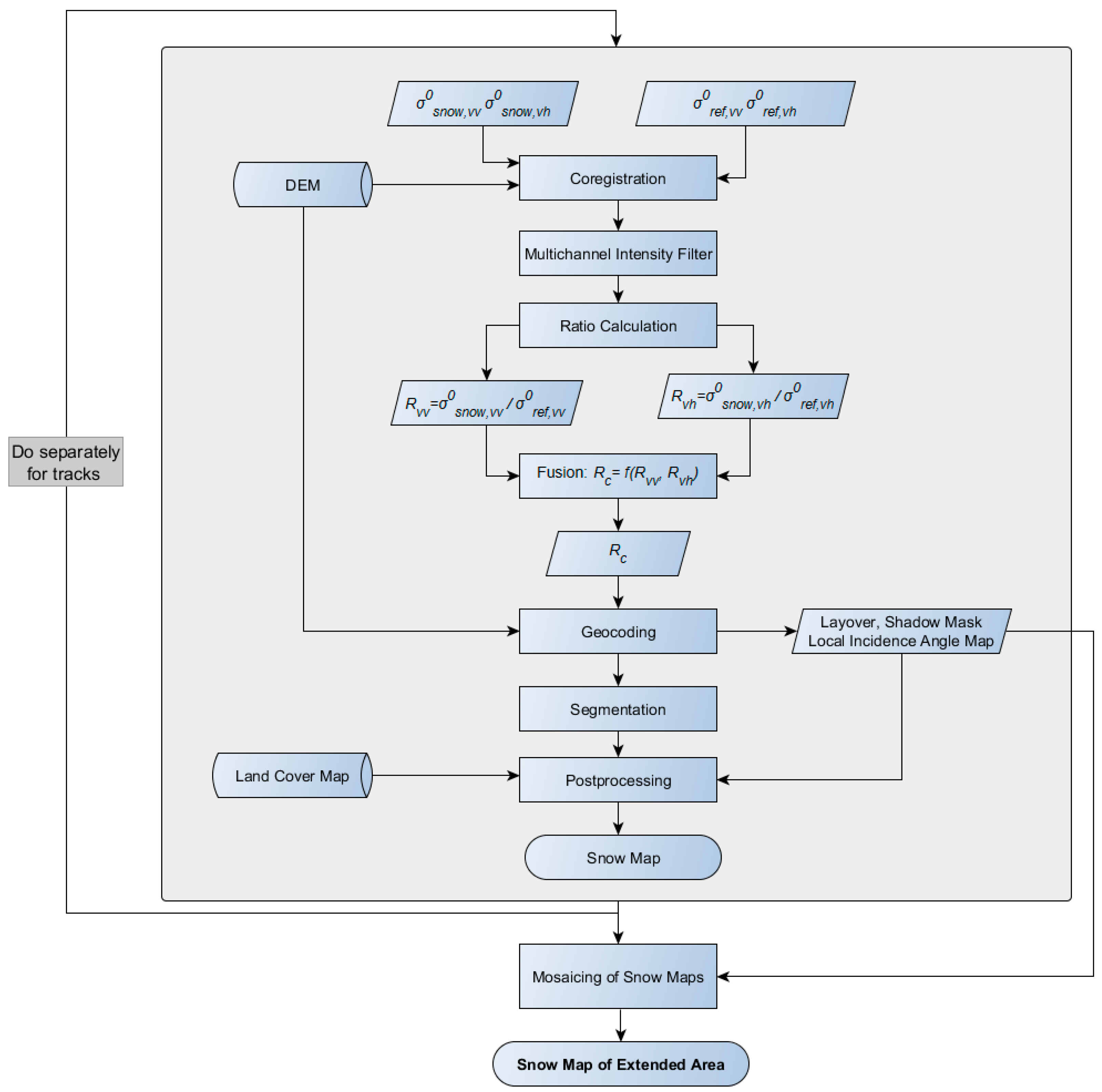
3.1. Classification Algorithm

Change detection procedures are commonly applied for retrieving snowmelt areas from SAR backscatter images [9,10,11,12,13,14]. This is an efficient means for reducing the impact of topography. The ratio of backscatter intensity of the SAR image with melting snow (${\sigma }_{snow}^0$) versus a reference image (${\sigma }_{ref}^0$) of the same satellite track is computed for detecting the reduced backscatter signal of melting snow areas. Threshold-based segmentation is applied to separate snow-covered and snow-free surfaces. Preferably, the reference image is the average of multiple SAR images from dates with surfaces that are snow-free and/or covered by dry snow. Stacking multiple images reduces speckle and helps to suppress the impact of temporal variations in backscatter in the reference scenes.

As a first step in the processing line, the snow image and reference images in radar geometry (Figure 1) are calibrated to radar brightness [18] and precisely co-registered to a pre-selected master image of the same track, using the orbit data and a DEM [30]. Due to the high accuracy of the S1 orbit data, geolocation at sub-pixel accuracy is achieved [20]. In the next step, the speckle-related uncertainty is reduced by applying a multichannel SAR intensity filter [31]. This filter optimally reduces speckle while preserving the intensity and spatial resolution of the individual channels. In the filtering process, $M$ new images $J_k$ are produced by linearly combining $M$ co-registered intensity images $I_i$, with $1 \le i \le M$. For intensity images with the same number of looks, $L$, the following formulation for the filter is valid [31]:

$$J_k= \frac{{\sigma }_k}{M}{\displaystyle \sum }_{i=1}^M\frac{I_i}{{\sigma }_i} , 1 \le k \le M$$

(1)

where ${\sigma }_k$ is the intensity in channel $k$ of the filtered image, and ${\sigma }_i$ is the mean intensity in the channel $i$ of the unfiltered image. The mean intensity in the filtered images is unbiased while the loss in spatial detail is minimal. An estimate of the local mean intensity is obtained by averaging the intensity values in a local window around each pixel. We apply the filter over windows of 7 × 7 pixels, using the stack of multi-temporal SLC images in the two polarizations. If all pixels in a window with $N$ pixels are spatially uncorrelated, the resulting equivalent number of looks, $ENL$, in the filtered image is:

$$ENL= \frac{M N L }{M+N-1}$$

(2)

Taking into account the difference in spatial resolution of the IW mode data in LOS and azimuth, we perform block averaging over 16 × 4 (LOS × azimuth) pixels of the SLC images before applying the multichannel filter. The averaged pixels have a size of about 55 m in azimuth and 58 m in ground range at 40° incidence angle. We estimated the equivalent number of looks by extracting the mean and variance of intensity over distributed targets with uniform surface properties extending over several hundred pixels. For the 16 × 4 block averaged pixels, the $ENL$ is 26. Applying the multichannel intensity filter increases $ENL$ significantly while maintaining the pixel size. Using one snow image and one reference image (dual channel each) we obtain after filtering $ENL=106$, and, using three reference images, $ENL=202$. For the reference images, further speckle reduction is achieved by using averages compiled from backscatter images of multiple dates.

The ${\sigma }^0$-ratio of the snow image versus the reference image is computed separately for the VV and VH channels and transformed to a logarithmic scale (dB). The statistical analysis shows a comparatively high degree of correlation between the VV and VH ratio images, with typical values of the correlation coefficient ($\rho$) of $0.85 \le \rho \le 0.90$ for different study areas. This suggests that the two-dimensional feature space, spanned by the VV and VH ratio channels, can be reduced to a one-dimensional ratio image before performing the segmentation. For fusion of the two channels, we use the weighted average of the VV and VH ratio. Experimental backscatter data and theory show reduced separability of the two classes for co-polarized backscatter at low local incidence angles (below about 30°) [25,29]. The separability in cross-polarized backscatter data, on the other hand, decreases only slightly towards low incidence angles.

Angular trends of multitemporal backscatter ratios for Sentinel-1 data are shown in Figure 2 for wet snow areas and snow-free surfaces in three study areas. Snow masks derived from Landsat images were used to extract the VV-polarized ($R_{vv}$) and VH-polarized ($R_{vh}$) backscatter ratios for the two classes. Details on the data sets and the procedures for this analysis are presented in Section 3.2 and Section 3.3. The ratios of snow-free surfaces show small angular variations, whereas the wet snow ratios change significantly. The differences between snow/snow-free classes decrease for both $R_{vv}$ and $R_{vh}$ from mid-range angles towards large angles. The separability between the two classes decreases significantly towards lower local incidence angles for $R_{vv}$, and less for $R_{vh}$. Taking into account this angular behavior, we apply the following relation for merging $R_{vv}$ and $R_{vh}$ ratios in order to create a combined single channel, $R_c$:

$$R_c=W R_{vh}+\left(1-W\right) R_{vv}.$$

(3)

The weight ($W$) varies with the local incidence angle ($\theta$) applying the following rule:

$$\begin{array}{c}IF \left(\theta <{\theta }_1\right) \to \left\{W=1.0\right\},\\ IF \left({\theta }_1 \le \theta \le {\theta }_2\right) \to \left\{W=k \left[1+ \raisebox{1ex}{$\left({\theta }_2-\theta \right)$}\!\left/ \!\raisebox{-1ex}{$\left({\theta }_2- {\theta }_1\right)$}\right.\right]\right\},\\ IF \left(\theta >{\theta }_2\right) \to \left\{W=k\right\}.\end{array}$$

(4)

For the data sets in this study, we use $k=0.5$, ${\theta }_1=20°$, ${\theta }_2=45°$. This means that $R_{vv}$ and $R_{vh}$ have the same weight for $\theta \ge 45°$. For $\theta <45°$, the weight of $R_{vv}$ decreases gradually, vanishing at $\theta =20°$. We limit the local incidence angles for snow mapping to the range $15°\le \theta \le 75°$. At lower angles, the surface resolution in range decreases significantly. At higher local incidence angles, the signal-to-noise ratio for targets with low reflectivity such as wet snow is quite small. Furthermore, for steep fore-slopes and near-grazing incidence, possible errors in the DEM used for geocoding become critical.

Terrain corrected geocoding is performed for the ratio image using precise orbit data. In addition, maps of the local incidence angle and masks of layover and radar shadow are generated by SAR image simulation using orbit and imaging parameters and a Digital Elevation Model as input. For the data presented in this paper we use the Digital Elevation Model over Europe (EU-DEM), which is a 3D raster data set with elevations captured at 1 arc second postings, corresponding to about 30 m [32]. For the standard snow product we are resampling the $R_c$ ratio image to a 100 m grid in UTM projection. The segmentation rule ($R_c<THR)$ for discriminating wet snow versus dry snow and snow-free areas is applied to the geocoded $R_c$ ratio image, using a threshold of $THR=-2 dB$. The selection of this threshold value is based on histograms of the ratio values for the two classes.

Post-processing includes the application of a 3 × 3 median filter to eliminate single outlier pixels, and the use of land cover maps to exclude dense forests and water surfaces. Forest cover and water bodies are extracted from the digital Landsat based maps of Hansen et al. [33] with 30 m resolution. In addition, we use the SRTM Water Body Data Set [34] for complementing the water mask by adding the river courses.

3.2. Landsat Maps of Snow Extent

In order to assess the quality of S1 based snow maps, we generated maps of snow extent from Landsat data over study areas in the Alps and in Iceland. Due to widespread cloudiness in these regions during the snowmelt seasons, the choice of suitable Landsat images for comparison with S1 snow maps is rather limited. The acquisition time, geographic location and solar elevation of the used Landsat scenes are specified in

Table 2. Information on the Landsat scenes used for comparison with S1 snow maps. Latitude, longitude and sun elevation refer to the scene center.

Study Area	Satellite	Date & Time (UTC)	Lat/Lon	Sun Elev.
A1, Tröllaskagi, Iceland	Landsat-8	27 June 2015 12:45	65.59° N/19.98° W	47.3°
A2, Ötztal Alps, Austria	Landsat-7	5 June 2015 10:03	47.45° N/11.02° E	61.4°
A3, Swiss Alps	Landsat-7	3 June 2015 10:16	46.03° N/7.39° E	62.1°

.

The images cover the Tröllaskagi Peninsula in northern Iceland and two subareas of the Alps. The Iceland image is cloud-free. The image of the Swiss Alps contains a few small cumulus clouds. The image of the Ötztal Alps shows a substantial number of scattered cumulus clouds, mainly over snow-free mountain slopes. Clouds of this type can be well detected by means of visible and short-wave infrared reflectance. We use thresholds in Landsat-7 bands 3 and 5 for cloud screening. Cloud shadows are identified visually by mapping dark pixels in the neighborhood of the clouds, taking into account the direction of solar illumination. The resulting cloud masks include the clouds and the cloud shadows.

Landsat-7 images are impaired by data gaps due to failure of the SLC. In order to minimize the impact of the SLC failure, we restrict the analysis to the central parts of the images, which are only slightly affected by this failure and, exclude the missing lines for the statistical comparison.

For generating the Landsat snow maps, we apply a binary algorithm with threshold-based segmentation in normalized difference snow index ($NDSI$) images, using as threshold value of $NDSI=0.4$, as applied for generating Landsat climate data records on snow extent [35]. The $NDSI$ is computed from top-of-atmosphere reflectances:

$$NDSI= \frac{R\left(VIS\right)-R\left(SWIR\right)}{R\left(VIS\right)+R\left(SWIR\right)}$$

(5)

For the Landsat-7 Enhanced Thematic Mapper (ETM+) we use the visible (VIS) band 2 (0.52–0.60 μm) and the shortwave infrared (SWIR) band 5 (1.55–1.75 μm), for the Landsat-8 Operational Land Imager (OLI), the band 3 (0.53–0.59 μm) and the band 6 (1.57–1.65 μm). The binary snow map is posted at 30 m pixel size in UTM projection, corresponding to the pixel size of the Landsat images.

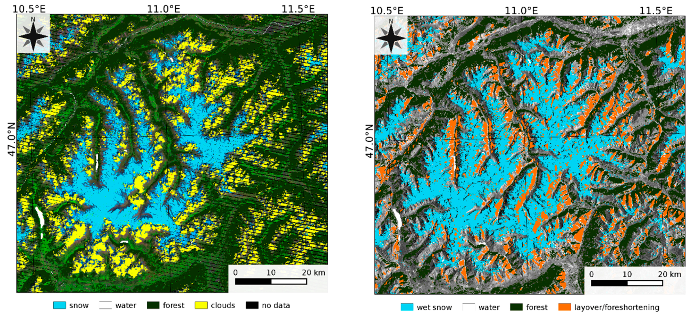
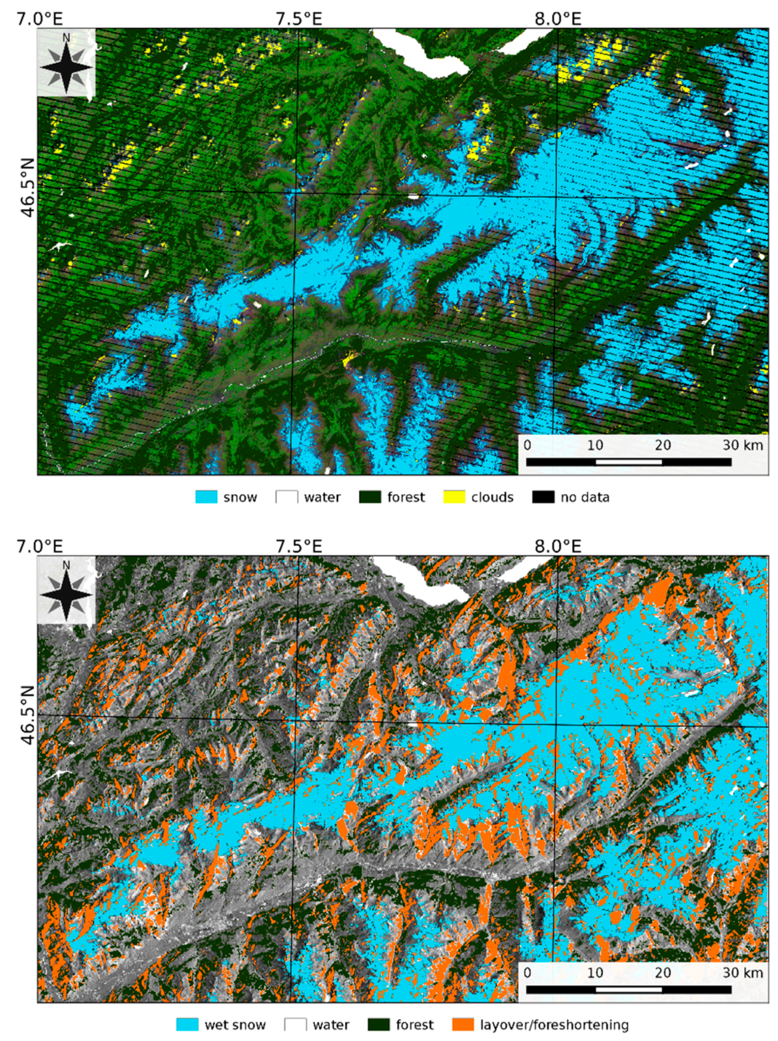
3.3. Comparison of Sentinel-1 and Landsat Snow Maps

For discussing the performance of S1 snow classification, we use the Landsat snow maps as reference. Landsat snow maps are frequently used as benchmarks for cross-sensor snow map validation [36] so that the S1 snow maps can be evaluated in relation to common snow-products.

The three study areas for comparison of Landsat and S1 snow maps cover mountainous terrain. The two Alpine areas extend over an elevation range of about 3500 m, more than twice the range at the Tröllaskagi Peninsula where the highest peak reaches 1538 m in elevation. In the Alpine study areas, the snowline on the selected dates was located above the tree line. The Iceland area lacks a forest cover.

Dates in late spring were selected for the intercomparison when the snow cover was melting up to the highest elevations. Suitable Landsat images are not available on exactly the same day as the S1 images. For the Iceland area (A1), the time difference is only one day, whereas for the Alpine areas the Landsat images were acquired 3 days later (A2), and 4 days earlier (A3), respectively, than the S1 image (Table 2 and

Table 3. Information on Sentinel-1 images used for comparison with Landsat snow maps. The incidence angle, $\theta$, refers to a horizontal surface in the center of each area.

Study Area	Date & Time UTC	Orbit Heading	Track Nr.	θ
A1, Tröllaskagi, Iceland	26 June 2015 07:41	Descending	9	40°
A2, Ötztal Alps, Austria	2 June 2015 05:26	Descending	168	37°
A3, Swiss Alps	7 June 2015 05:35	Descending	66	42°

). For the area A1, the impact of the time difference is probably very small, as the good agreement between the Landsat and S1 snow maps shows (Figure 3).

Figure 3, Figure 4 and Figure 5 show the binary Landsat and S1 snow maps at 100 m pixel size. In order to match the grid size of the S1 maps for the statistical comparison, the binary 30 m Landsat snow pixels are aggregated into pixels of 100 m size. This provides an estimate of fractional snow cover at 100 m scale, representing an upper estimate because the $NDSI$ threshold value of 0.4, used for the binary snow classification, corresponds to a cut-off value of about 50% snow cover [35,36]. For the statistical comparison (

Table 4. Confusion matrix for the classes snow (S) and snow-free (F) in the 3 study areas, for snow classification based on Landsat (LS) and Sentinel-1 (S1) data. S1 results are shown for snow maps based on the ratios $R_{vv}$, $R_{vh}$ , and $R_c$. AR —overall agreement rate ($0.0\le AR\le 1.0$).

Area		Rvv			Rvh			Rc
		S1-S	S1-F	AR	S1-S	S1-F	AR	S1-S	S1-F	AR
A1	LS-S	92.8	7.2		92.6	7.4		94.6	5.4
	LS-F	2.0	98.0		0.2	99.8		0.2	99.8
				0.954			0.962			0.972
A2	LS-S	80.7	19.3		94.5	6.4		94.7	5.3
	LS-F	4.2	95.8		5.3	94.7		3.2	97.8
				0.882			0.946			0.962
A3	LS-S	72.9	27.1		93.6	6.4		92.2	7.8
	LS-F	6.5	93.5		4.6	95.4		3.1	96.9
				0.832			0.945			0.946

), we generate a binary Landsat snow map with 100 m pixel size by assigning all pixels with fractional snow extent $\ge 75 \%$ to the snow class. This map is also used for defining snow/snow-free areas to extract the S1 backscatter ratios for Figure 2. Areas with clouds in Landsat images and areas with layover, foreshortening (S1 local incidence angle $\theta <15°$), backslopes with $\theta >75°$, and dense forests in S1 images are masked out.

For compiling the confusion matrix between Landsat and S1 snow classification (Table 4), the total pixel number is normalized according to the Landsat-based classification result, assigning the value 100 to each class. This normalization enables a direct comparison of the performance for the different study areas and for the different ratio images. The overall agreement rate ($0.0\le AR\le 1.0$) shows for areas A1 and A2 the best agreement for the combined ratio ($R_c$) and a small decline for $R_{vh}$. For A3, the performance of $R_c$ and $R_{vh}$ is the same. The drop-off in the $AR$ of $R_{vv}$ is significant for the areas A2 and A3. We tested the application of different threshold values for segmentation in the $R_{vv}$ images, but this does not result in improvements. The lower performance of $R_{vv}$ for snow detection is in accordance with the smaller difference between the ratios of snow-covered and snow-free areas, in particular at lower incidence angles (Figure 2).

Tröllaskagi Peninsula has the highest overall agreement rate (0.97), followed by Ötztal Alps (0.96) and Swiss Alps (0.95). The time difference of three (Ötztal), respectively four (Swiss Alps) days, between the Landsat and S1 snow maps may play a role. Moreover, the two Alpine areas have steeper topography than the Tröllaskagi Peninsula, as is obvious from the higher fractions of layover and foreshortening in Figure 4 and Figure 5 versus Figure 3. The impact of topography seems to be substantial for the $R_{vv}$ based classification, as indicated by the lower AR values for Ötztal and the Swiss areas.

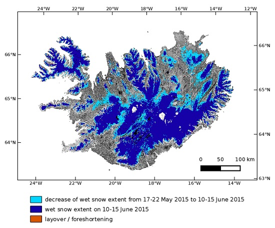
4. Sentinel-1 Snow Maps of Iceland and European Alps

Figure 6 and Figure 7 show snowmelt maps over large areas on different dates. The pixel size is 100 m, providing better spatial resolution than the snow maps derived from medium resolution optical sensors (e.g., MODIS [36]). In case of overlapping tracks, we select the pixel with the local incidence angle closest to $\theta =45 °$, in order to fetch the angle with the better separability between the snow and snow-free classes.

For Iceland (Figure 6), snow maps posted in 100 m UTM were compiled for two epochs: (1) based on S1 IW images of 17 May (track 118), 19 May (track 147), 22 May 2015 (track 016); (2) based on S1 IW images of 10 June, 12 June and 15 June 2015 (same tracks as in May). Between the two epochs, the snowline ascended from about 600 m to 800 m in elevation. Above about 1600 m altitude, the accumulation areas on the ice caps Vatnajökull and Hofsjökull were still dry in the June images. The dry snow areas show little temporal variability in backscatter and therefore can be well identified in the ratio images.

Snow maps over the Alps (Figure 7) are shown for three epochs based on S1 IW images of: (1) 20, 21, 22 and 23 April 2015; (2) 14, 15, 16 and 17 May 2015; (3) 1, 2, 3 and 4 July 2015. The track numbers are 66, 88, 95 and 117. The digital radar-based map, displayed in Figure 7, comprises 43 million pixels of about 100 m size in geographic map projection. The SLC database used for compiling the snow map of a single track comprises about 20 GB, for the time series including reference images about 100 GB. On date 1 (20–23 April), melting snow surfaces extended up to 3000 m altitude, and on date 2, (14–17 May), to 3500 altitude. In the combined snow map, the dry snow areas are superposed by melting snow areas of later dates.

5. Discussion

The investigations demonstrate the excellent capability of the Sentinel-1 mission for operational monitoring of snowmelt areas. The proposed algorithm, based on change detection in multitemporal SAR images, represents an extension to previously applied procedures for wet snow mapping. It exploits the advanced technical features of the S1 SAR sensor. Of particular benefit for the quality of the snowmelt area maps are the high instrument stability and the high spatial resolution across the comparatively wide swath of the IW mode [21]. The electronic azimuth scanning by means of the TOPSAR operation, harmonizing the performance in along-track direction and reducing scalloping effects, offers significant improvements in terms of radiometric quality compared to the conventional ScanSAR operation mode [3]. Due to the high spatial resolution of S1 SAR and the application of multichannel filtering in the snow mapping algorithm, the speckle-related uncertainty for the multi-temporal ratio images is very low.

Another beneficial feature for snow mapping is the regular acquisition of dual polarization (VV-VH) IW mode data, being used as standard operation scenario over many land areas [37]. Co-polarized channel data are the preferred option for interferometric applications, a main application field of the S1 mission. On the other hand, for retrieving snowmelt areas, the added value of cross-polarized data is significant, in particular in regions with steep topography. Thanks to the moderate angular dependence of backscatter, cross-polarized data offer good separability of wet snow and snow-free surfaces also on fore-slopes. For co-polarized data, the separability decreases significantly towards low incidence angles.

For assessing the accuracy of the S1 snow maps, we performed pixel-wise comparisons with Landsat-based snow maps. The results cannot be exactly translated into error numbers for the S1 snow maps because Landsat snow maps also show sensor specific features [35], and the dates of the Landsat and S1 snow maps differ by up to four days. Even so, the overall agreement rate between the Landsat and S1 classifications ranges from 0.95 to 0.97 for the various test sites (Table 4), confirming the good quality of both products that are derived from independent data sources. These numbers indicate significant improvements for SAR snow mapping by Sentinel-1 compared to previous snow cover products that are based on co-polarized SAR data of various satellite missions [11,12,13,14].

The comparison with Landsat snow maps reveals a slight trend for underestimation of snow extent for S1. This refers mainly to pixels with patchy snow cover where the signal contribution of snow-free surface dominates in SAR images, whereas the NDSI-based binary classifier separates the two classes at about 50% fractional snow cover [35,36].

For dense coniferous forest, common in the European Alps, reliable snow mapping with C-band SAR is not feasible because the radar signal is largely dominated by scattering in the canopy [38]. Therefore, we apply a land cover mask to exclude forested areas for snow retrievals over the Alps. Forests in Nordic areas are less dense, which offers the possibility to detect melting snow in open forests [39]. This could be a topic for further studies on the application of S1 for snow mapping.

6. Conclusions

The Sentinel satellite missions are dedicated to long-term routine observations for operational services in a wide range of applications. The data are also of great benefit to the Earth science community. Each Sentinel mission is based on a constellation of two identical satellites. By now, the first satellites of the Sentinel-1, -2, and -3 missions are in orbit. In this paper, we report on the features and performance of an algorithm for generating maps of snowmelt area based on radar images of the Sentinel-1 mission.

The nominal operation mode of the S1 SAR sensor for land areas is the Interferometric Wide swath (IW) mode, which offers high radiometric accuracy and high spatial resolution and covers a swath of 250 km width. These are important attributes for snow retrievals that are based on backscatter signals. Of benefit for snowmelt retrievals, in particular in regions with steep topography, is also the acquisition of cross-polarized data, helping to compensate for the reduced sensitivity of co-polarized data for detection of wet snow on fore-slopes. The comparison with snow maps derived from high resolution optical sensors confirms the high quality of the S1 snow cover maps. In particular, during the snowmelt period, when the snow extent is subject to rapid changes, the high temporal revisit of the S1 mission is of great value for hydrology, water management, flood forecasting and support of land surface process modeling. The revisit time of a single S1 satellite operating in IW mode is about four days in mid-latitudes and about two days in high latitudes. After deployment of the Sentinel-1B satellite, scheduled for launch on 22 April 2016, the revisit time will improve by a factor of two.

Whereas a main advantage of C-band SAR for snow mapping is the feasibility to penetrate clouds, the sensitivity to dry snow cover is rather limited. Therefore, the synergy with optical sensors is needed for a comprehensive observing system on snow extent. The Sentinel-2 and Sentinel-3 missions of the Copernicus program offer excellent capabilities for this task. Sentinel-2 is a polar-orbiting, multispectral imaging mission with 13 spectral bands (from 443 nm to 2190 nm wavelength) and spatial resolution of 10 m, 20 m and 60 m in the various channels, covering a swath of 290 km width [40]. With two satellites, the coverage by repeat orbits will be five days, disregarding cloud cover. The Sentinel-3 mission is equipped with a dual frequency synthetic aperture radar altimeter and two medium-resolution optical sensors: an imaging spectrometer, the Ocean Land Color Instrument (OLCI), and a dual-view multispectral radiometer, the Sea Land Surface Temperature Radiometer (SLSTR) [41]. After full deployment, the Sentinel-3 mission offers daily complete coverage in mid and high latitudes. Whereas the optical observation sequences for dynamic phenomena, such as seasonal snow, are strongly impaired by cloud cover, Sentinel-1 provides regular revisits at high temporal sequence, well-matched for capturing rapid changes due to snowmelt. The investigations reported here highlight the great potential of S1 for operational monitoring of snowmelt areas and for supporting multi-sensor snow cover mapping.

References

1. Aschbacher, J.; Milagro-Peréz, M.P. The European Earth monitoring (GMES) programme: Status and perspectives. Remote Sens. Environ. 2012, 120, 3–8. [Google Scholar] [CrossRef]
2. Copernicus—Application Domains. Available online: http://www.copernicus.eu/main/application-domains (accessed on 20 February 2016).
3. Torres, R.; Snoeij, P.; Geudtner, D.; Bibby, D.; Davidson, M.; Attema, E.; Potin, P.; Rommen, B.; Floury, N.; Brown, M.; et al. GMES Sentinel-1 mission. Remote Sens. Environ. 2012, 120, 9–24. [Google Scholar] [CrossRef]
4. Fletcher, K. Sentinel-1: ESA’s Radar Observatory Mission for GMES Operational Services; ESA SP-1322/1; ESA-ESTEC: Noordwijk, The Netherlands, 2012; p. 83. [Google Scholar]
5. Pedersen, L.T.; Saldo, R.; Fenger-Nielsen, R. Sentinel-1 results: Sea ice operational monitoring. In Proceedings of the IEEE IGARSS, Milan, Italy, 26–31 July 2015; pp. 2828–2831.
6. Nagler, T.; Rott, H.; Hetzenecker, M.; Wuite, J.; Potin, P. The Sentinel-1 Mission: New opportunities for ice sheet observations. Remote Sens. 2015, 7, 9371–9389. [Google Scholar] [CrossRef]
7. Potin, P.; Rosich, B.; Roeder, J.; Bargellini, P. Sentinel-1 mission operations concept. In Proceedings of the IEEE IGARSS, Québec, QC, Canada, 13–18 July 2014; pp. 1465–1468.
8. Malenovský, Z.; Rott, H.; Cihlar, J.; Schaepman, M.E.; García-Santos, G.; Fernandes, R.; Berger, M. Sentinels for Science: Potential of Sentinel-1, -2, and -3 missions for scientific observations of ocean, cryosphere and land. Remote Sens. Environ. 2012, 120, 91–101. [Google Scholar] [CrossRef]
9. Baghdadi, N.; Gauthier, Y.; Bernier, M. Capability of multitemporal ERS-1 SAR data for wet snow mapping. Remote Sens. Environ. 1997, 60, 174–186. [Google Scholar] [CrossRef]
10. Baghdadi, N.; Gauthier, Y.; Bernier, M.; Fortin, J.P. Potential and limitations of RADARSAT SAR data for wet snow monitoring. IEEE Trans. Geosci. Remote Sens. 2000, 38, 316–320. [Google Scholar] [CrossRef]
11. Nagler, T.; Rott, H. Retrieval of wet snow by means of multitemporal SAR data. IEEE Trans. Geosci. Remote Sens. 2000, 38, 754–765. [Google Scholar] [CrossRef]
12. Nagler, T.; Rott, H.; Glendinning, G. Snowmelt runoff modelling by means of RADARSAT and ERS SAR. Can. J. Remote Sens. 2000, 26, 512–520. [Google Scholar] [CrossRef]
13. Luojus, K.P.; Pulliainen, J.; Metsamaki, S.; Hallikainen, M. Snow-covered area estimation using satellite radar wide-swath images. IEEE Trans. Geosci. Remote Sens. 2007, 45, 978–989. [Google Scholar] [CrossRef]
14. Nagler, T.; Rott, H.; Malcher, P.; Müller, F. Assimilation of meteorological and remote sensing data for snowmelt runoff forecasting. Remote Sens. Environ. 2008, 112, 1408–1420. [Google Scholar] [CrossRef]
15. Longepe, N.; Allain, S.; Ferro-Famil, L.; Pottier, E.; Durand, Y. Snowpack characterization in mountainous regions using C-Band SAR data and a meteorological model. IEEE Trans. Geosci. Remote Sens. 2009, 47, 406–418. [Google Scholar] [CrossRef]
16. CryoLand-Copernicus Service Snow and Land Ice. Available online: http://www.cryoland.eu (accessed on 14 April 2016).
17. Key, J.; Drinkwater, M.; Ukita, J. (Eds.) IGOS Cryosphere Theme Report; WMO/TD-1405; WMO: Geneva, Switzerland, 2007; p. 124.
18. Miranda, N.; Meadows, P.J. Radiometric Calibration of S-1 Level-1 Products Generated by the S-1 IPF; ESA-EOPG-CSCOP-TN-0002; Technical Note. European Space Agency: Frascati, Italy, 2015; p. 13. Available online: https://sentinel.esa.int/documents/247904/685163/S1-Radiometric-Calibration-V1.0.pdf (accessed on 14 April 2016).
19. Sentinel-1 Team. Sentinel-1 User Handbook; GMES-S1OP-EOPG-TN-13-0001. European Space Agency: Frascati, Italy, 2013; p. 80. Available online: https://sentinel.esa.int/documents/247904/ 685163/Sentinel-1_User_Handbook (accessed on 14 April 2016).
20. Miranda, N.; Palumbo, G. Sentinel-1 Instrument and Product Performance Status. In Proceddings of the FRINGE 2015 Workshop, ESA-ESRIN, Frascati, Italy, 23–27 March 2015; Available online: http://seom.esa.int/fringe2015/files/presentation359.pdf (accessed on 18 February 2016).
21. Miranda, N.; Meadows, P.; Hajduch, G.; Pilgrim, A.; Piantanida, R.; Giudici, D.; Small, D.; Schubert, A.; Husson, R.; Vincent, P.; et al. The Sentinel-1A instrument and operational product performance status. In Proceedings of the IEEE IGARSS, Milan, Italy, 26–31 July 2015; pp. 2824–2827.
22. Knight, E.J.; Kvaran, G. Landsat-8 Operational Land Imager design, characterization, and performance. Remote Sens. 2014, 6, 10286–10305. [Google Scholar] [CrossRef]
23. Storey, J.; Choate, M.; Lee, K. Landsat 8 Operational Land Imager on-orbit geometric calibration and performance. Remote Sens. 2014, 6, 11127–11152. [Google Scholar] [CrossRef]
24. Shi, J.; Dozier, J. Inferring snow wetness using C-band data from SIR-C’s polarimetric synthetic aperture radar. IEEE Trans. Geosci. Remote Sens. 1995, 33, 905–914. [Google Scholar]
25. Mätzler, C. Applications of the interaction of microwaves with the natural snow cover. Remote Sens. Rev. 1987, 2, 259–387. [Google Scholar] [CrossRef]
26. Ulaby, F.T.; Long, D. Microwave Radar and Radiometric Remote Sensing; University of Michigan Press: Ann Arbor, MI, USA, 2014; p. 1016. [Google Scholar]
27. Reber, B.; Mätzler, C.; Schanda, E. Microwave signatures of snow crusts. Modeling and measurements. Int. J. Remote Sens. 1987, 8, 1649–1665. [Google Scholar] [CrossRef]
28. Floricioiu, D.; Rott, H. Seasonal and short-term variability of multifrequency, polarimetric radar backscatter of alpine terrain from SIR-C/X-SAR and AIRSAR data. IEEE Trans. Geosc. Rem. Sens. 2001, 39, 2634–2648. [Google Scholar] [CrossRef]
29. Strozzi, T.; Wiesman, A.; Mätzler, C. Active microwave signatures of snow covers at 5.3 and 35 GHz. Radio Sci. 1997, 32, 479–495. [Google Scholar] [CrossRef]
30. Sansosti, E.; Berardino, P.; Manunta, M.; Serafino, F.; Fornaro, G. Geometrical SAR image registration. IEEE Trans. Geosci. Remote Sens. 2006, 44, 2861–2870. [Google Scholar] [CrossRef]
31. Quegan, S.; Yu, J.J. Filtering of multichannel SAR data. IEEE Trans. Geosc. Rem. Sens. 2001, 39, 2373–2379. [Google Scholar] [CrossRef]
32. European Environment Agency. Digital Elevation Model over Europe (EU-DEM). Available online: http://www.eea.europa.eu/data-and-maps/data/eu-dem (accessed on 12 February 2016).
33. Hansen, M.C.; Potapov, P.V.; Moore, R.; Hancher, M.; Turubanova, S.A.; Tyukavina, A.; Thau, D.; Stehman, S.V.; Goetz, S.J.; Loveland, T.R.; et al. High-Resolution Global Maps of 21st-Century Forest Cover Change. Science 2013, 342, 850–853. [Google Scholar] [CrossRef] [PubMed]
34. SRTM Water Body Dataset. Available online: https://lta.cr.usgs.gov/srtm_water_body_dataset (accessed on 12 February 2016).
35. Crawford, C.J.; Manson, S.M.; Bauer, M.E.; Hall, D.K. Multitemporal snow cover mapping in mountainous terrain for Landsat climate data record development. Remote Sens. Environ. 2013, 135, 224–233. [Google Scholar] [CrossRef]
36. Crawford, C.J. MODIS Terra Collection 6 fractional snow cover validation in mountainous terrain during spring snowmelt using Landsat TM and ETM+. Hydrol. Process. 2015, 29, 128–138. [Google Scholar] [CrossRef]
37. Potin, P.; Rosich, B.; Miranda, N.; Grimont, P.; Bargellini, P.; Monjoux, E.; Martin, J.; Desnos, Y.-L.; Roeder, J.; Shurmer, I. Sentinel-1 mission status. In Proceedings of the IEEE IGARSS, Milan, Italy, 26–31 July 2015; pp. 2820–2823.
38. Karam, M.A.; Amar, F.; Fung, A.K.; Mougin, E.; Lopes, A.; Vine, D.M.L.; Beaudoin, A. A microwave polarimetric scattering model for forest canopies based on vector radiative transfer theory. Remote Sens. Environ. 1995, 53, 16–30. [Google Scholar] [CrossRef]
39. Koskinen, J.T.; Pulliainen, J.T.; Luojus, K.P.; Takala, M. Monitoring of snow cover properties during the spring melting period in forested areas. IEEE Trans. Geosci. Remote Sens. 2010, 48, 50–58. [Google Scholar] [CrossRef]
40. Drusch, M.; Del Bello, U.; Carlier, S.; Colin, O.; Fernandez, V.; Gascon, F.; Hoersch, B.; Isola, C.; Laberinti, P.; Martimort, P.; et al. Sentinel-2: ESA’s Optical High-Resolution Mission for GMES Operational Services. Remote Sens. Environ. 2012, 120, 25–36. [Google Scholar] [CrossRef]
41. Donlon, C.; Berruti, B.; Buongiorno, A.; Ferreira, M.-H.; Féménias, P.; Frerick, J.; Goryl, P.; Klein, U.; Laur, H.; Mavrocordatos, C.; et al. The Global Monitoring for Environment and Security (GMES) Sentinel-3 Mission. Remote Sens. Environ. 2012, 120, 37–57. [Google Scholar] [CrossRef]
Figure 1. Flow chart of the algorithm for retrieval of snowmelt area from Sentinel-1 Interferometric Wide swath mode data.
Remotesensing 08 00348 g001
Figure 2. Backscatter ratio (median, Mdn, 1st and 3rd quartile) for S1 VV- and VH- polarized channels in dependence of the local incidence angle, θ , for areas classified as snow-free and snow-covered in Landsat images (see Section 3.2): (a) test site A1: Tröllaskagi; (b) test site A2: Ötztal Alps; (c) test site A3: Swiss Alps.
Remotesensing 08 00348 g002
Figure 3. Snow map of Tröllaskagi Peninsula, Iceland. (Left) Snow extent (blue) derived from Landsat-8 image of 27 June 2015; white: water; background: Landsat-8 OLI bands 6, 5, 4. (Right) Wet snow extent (blue) derived from Sentinel-1 image of 26 June 2015; background: S1 amplitude image, VV-channel; orange: mask for layover and foreshortening.
Remotesensing 08 00348 g003
Figure 4. Snow map of the Ötztal mountain region, Eastern Alps of Austria and Italy. (Left) Snow extent (blue) derived from Landsat-7 image of 5 June 2015; yellow: clouds; white: water; background: Landsat-7 ETM+ bands 5, 4, 3. (Right) Wet snow extent (blue) derived from Sentinel-1 image of 2 June 2015; background: S1 amplitude image, VV-channel; orange: mask for layover and foreshortening.
Remotesensing 08 00348 g004
Figure 5. Snow map of Swiss Alps (Berne, Valais). (Top) Snow extent (blue) derived from Landsat-7 image of 3 June 2015; background: Landsat ETM+ bands 5, 4, 3; yellow: clouds; white: water. (Bottom) Snow extent (blue) derived from Sentinel-1 image of 7 June 2015; background: amplitude image, VV-channel; orange: mask for layover and foreshortening.
Remotesensing 08 00348 g005
Figure 6. Map of snowmelt area extent in Iceland, derived from Sentinel-1 data of 17, 19 and 22 May 2015 (Date 1) and 10, 12, and 15 June 2015 (Date 2). Light blue: decrease of snow extent between Date 1 and Date 2. Dark blue: snowmelt area on Date 2. Light grey: dry snow on ice caps; white: water surfaces; orange: mask of layover and foreshortening. Background: S1 SAR amplitude image, VV polarizations.
Remotesensing 08 00348 g006
Figure 7. Map of snowmelt area extent over the Alps, derived from Sentinel-1 data of 20 to 23 April 2015 (Date 1), 14 to 17 May 2015 (Date 2), 1 to 4 July 2015 (Date 3). Light blue: decrease of snow extent between Date 1 and Date 2. Dark blue: decrease of snow extent between Date 2 and Date 3; Purple: snowmelt area on Date 3. Black: water surfaces; orange: mask of layover and foreshortening. Background: S1 SAR amplitude image, VV polarizations.
Remotesensing 08 00348 g007