
A Spectral-Spatial Classification of Hyperspectral Images Based on the Algebraic Multigrid Method and Hierarchical Segmentation Algorithm


Abstract
:
1. Introduction
2. Materials and Methods
2.1. Hyperspectral Anisotropic Diffusion PDE
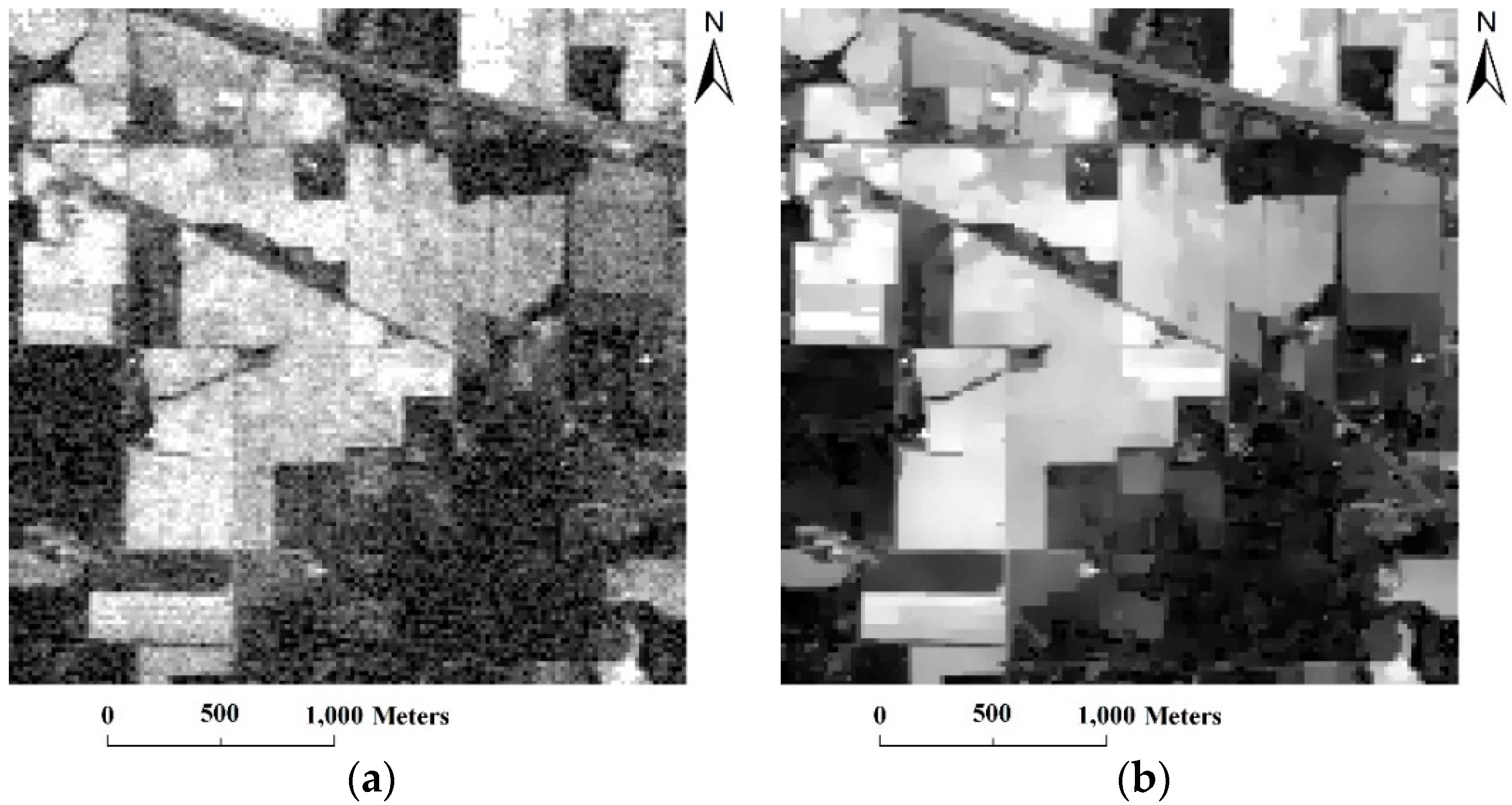
2.2. Multiscale Representation of Hyperspectral Imagery
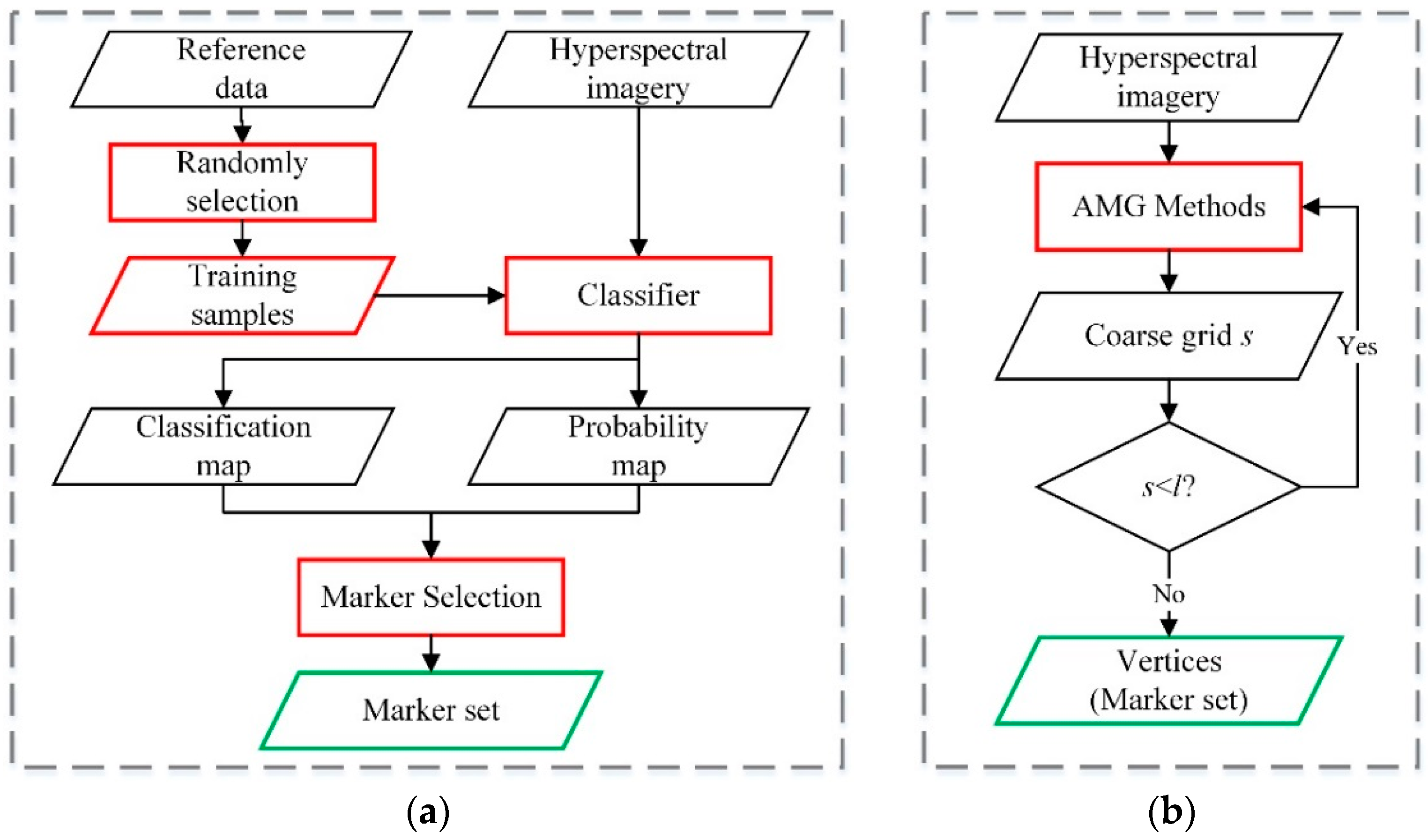
- The first step is the consecutive selection of a new set of from , where l is used to denote the current grid level with , where S is the coarsest grid. The set of vertices is sorted in decreasing order according to . Then, the first vertex of is initialized as the vertex in that has the highest mass. Finally, the set of vertices at grid l+1 can be obtained:where is a threshold value, and denotes the set difference between and . Note that , and in the finest grid are initialized as before, and we can compute the coarser grid according to the previous algorithm. Once the vertices of the finest coarse grid are constructed, we compute the masses in the next grid and the dependence degrees of the vertices in to the vertices in asandwhere is a measure of how much vertex depends on vertex .
- The second step is performed by connecting the vertices in to obtain , which can be realized first by computing for all the vertices in grid level and then connecting the vertices to obtain . Based on the Garlekin principle [34], the matrix of diffusion coefficients can be defined as the Garlekin operator , where denotes the restriction operator that maps vectors in a fine grid into a coarser one and is given bywhere is the interpolation operator, which is used to interpolate the intensity back to the finer grids and is given by
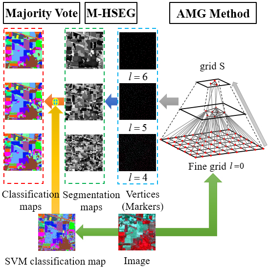
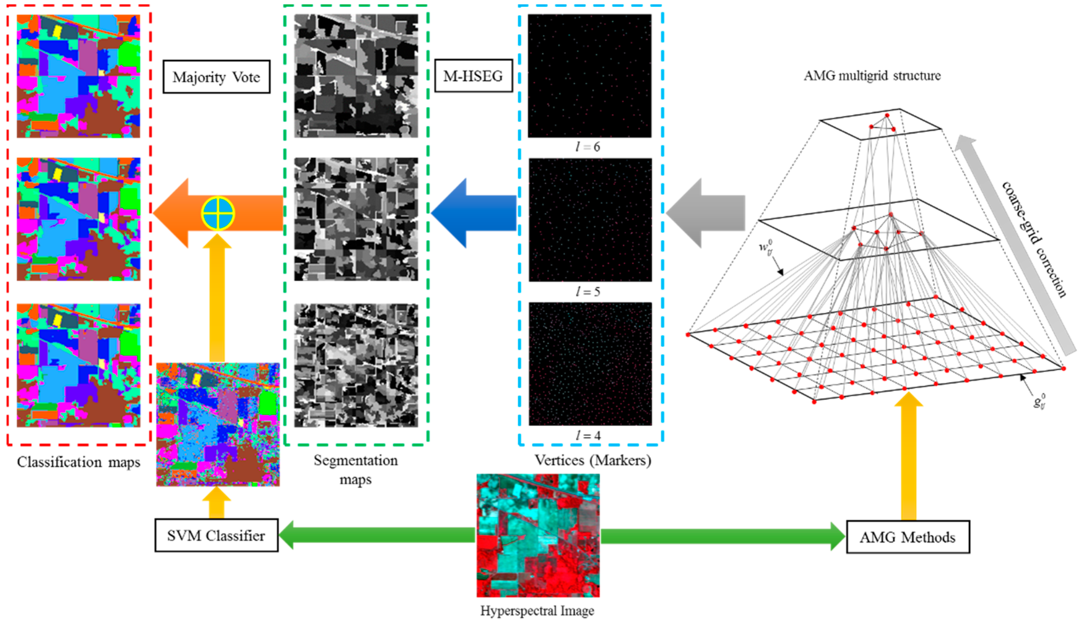
2.3. AMG-Derived M-HSEG Method
| Algorithm 1: AMG-derived M-HSEG Segmentation Algorithm |
| Input: An original hyperspectral image u and the coarsest grid level S. |
| Output: Segmentation maps |
|
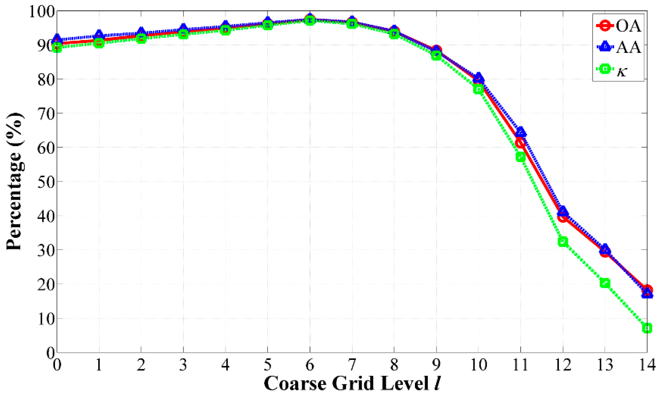
2.4. Selection of the Optimal Grid Level
3. Results
3.1. Parameter Settings and Evaluation Measures
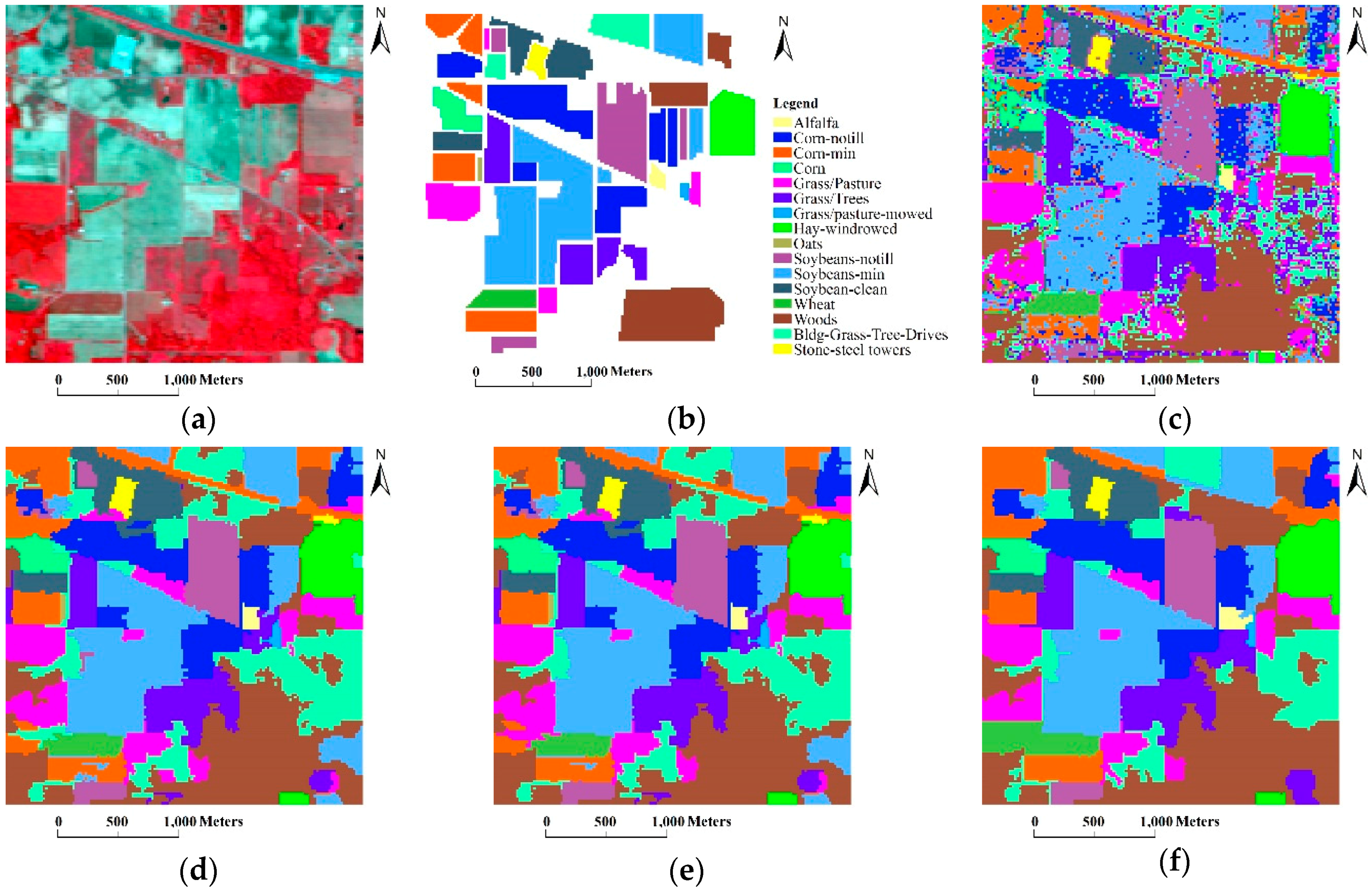
3.2. The Indian Pines Image (AVIRIS)
3.3. The Washington DC Image (HYDICE)
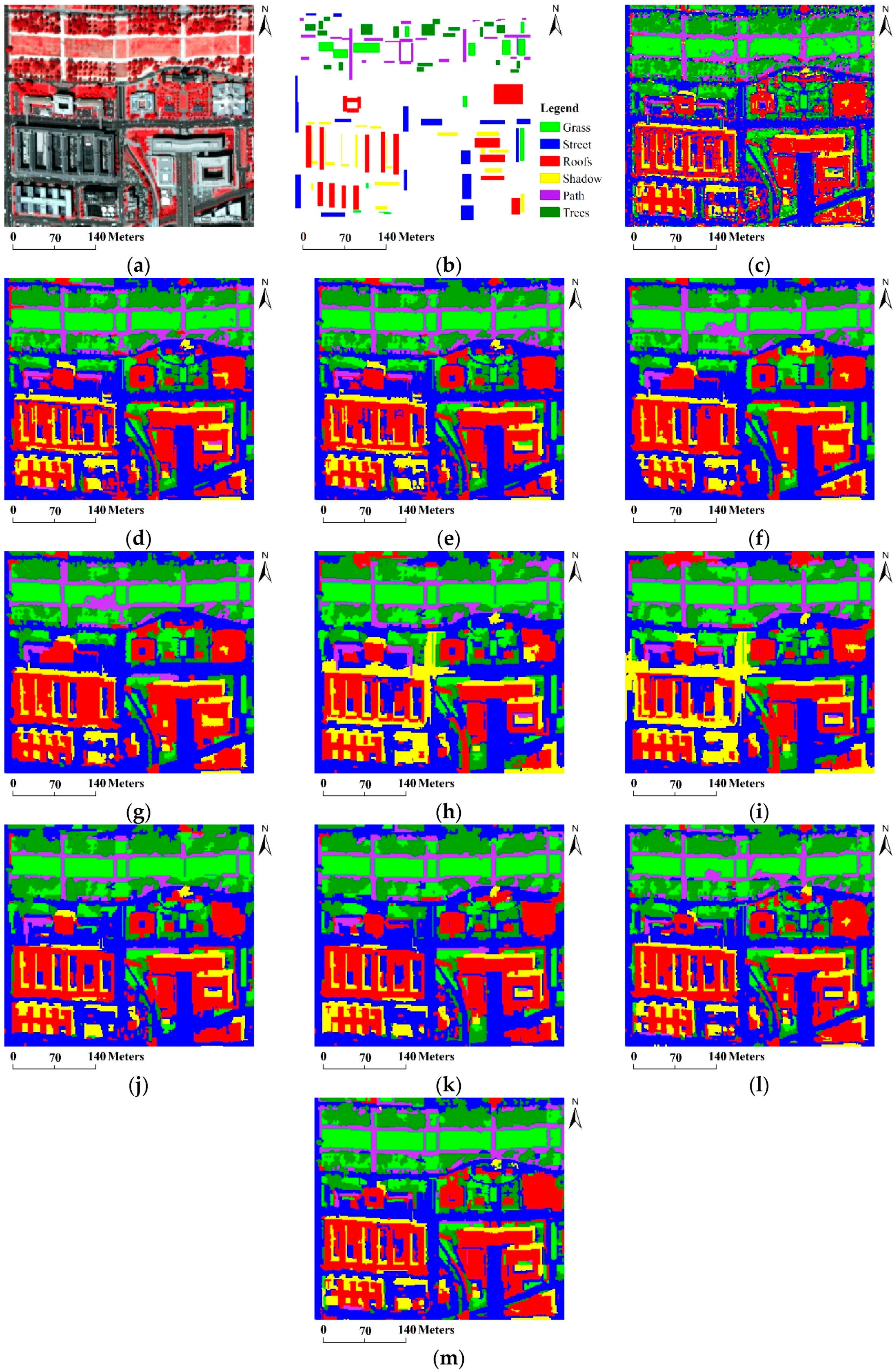
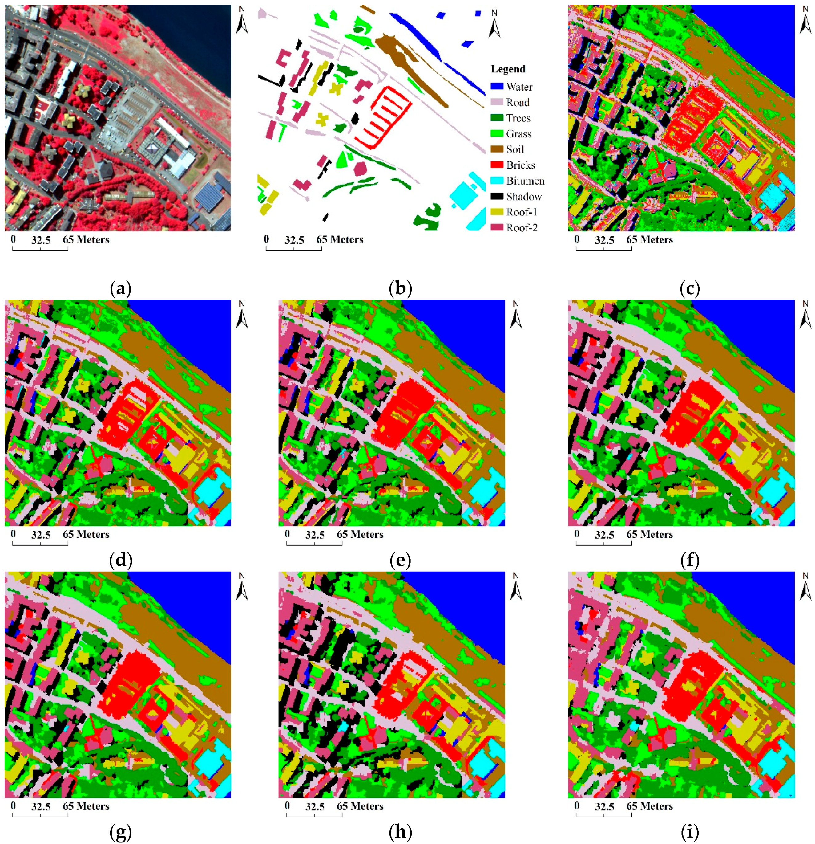
3.4. The Centre of Pavia Image (ROSIS)
4. Discussion
- (1)
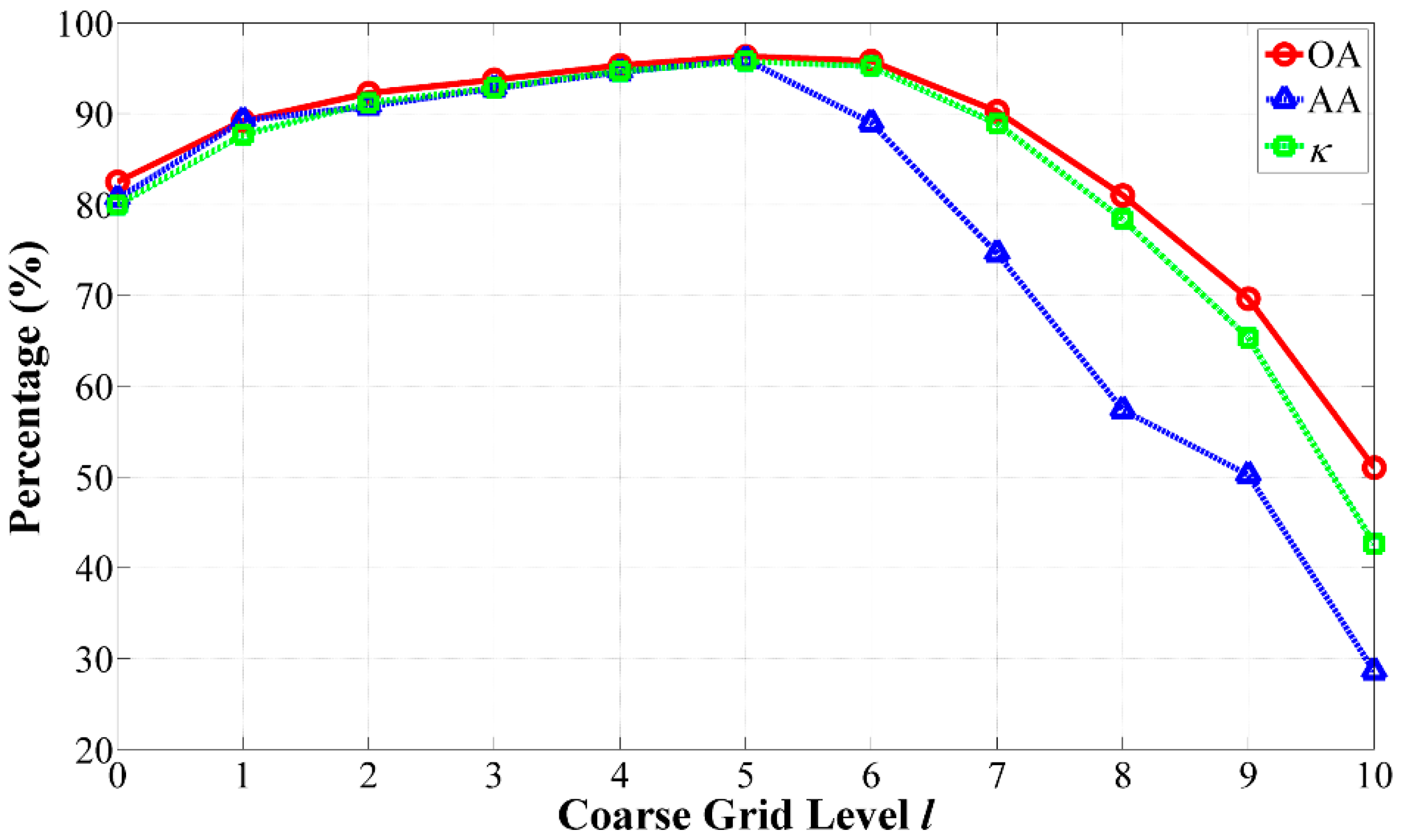
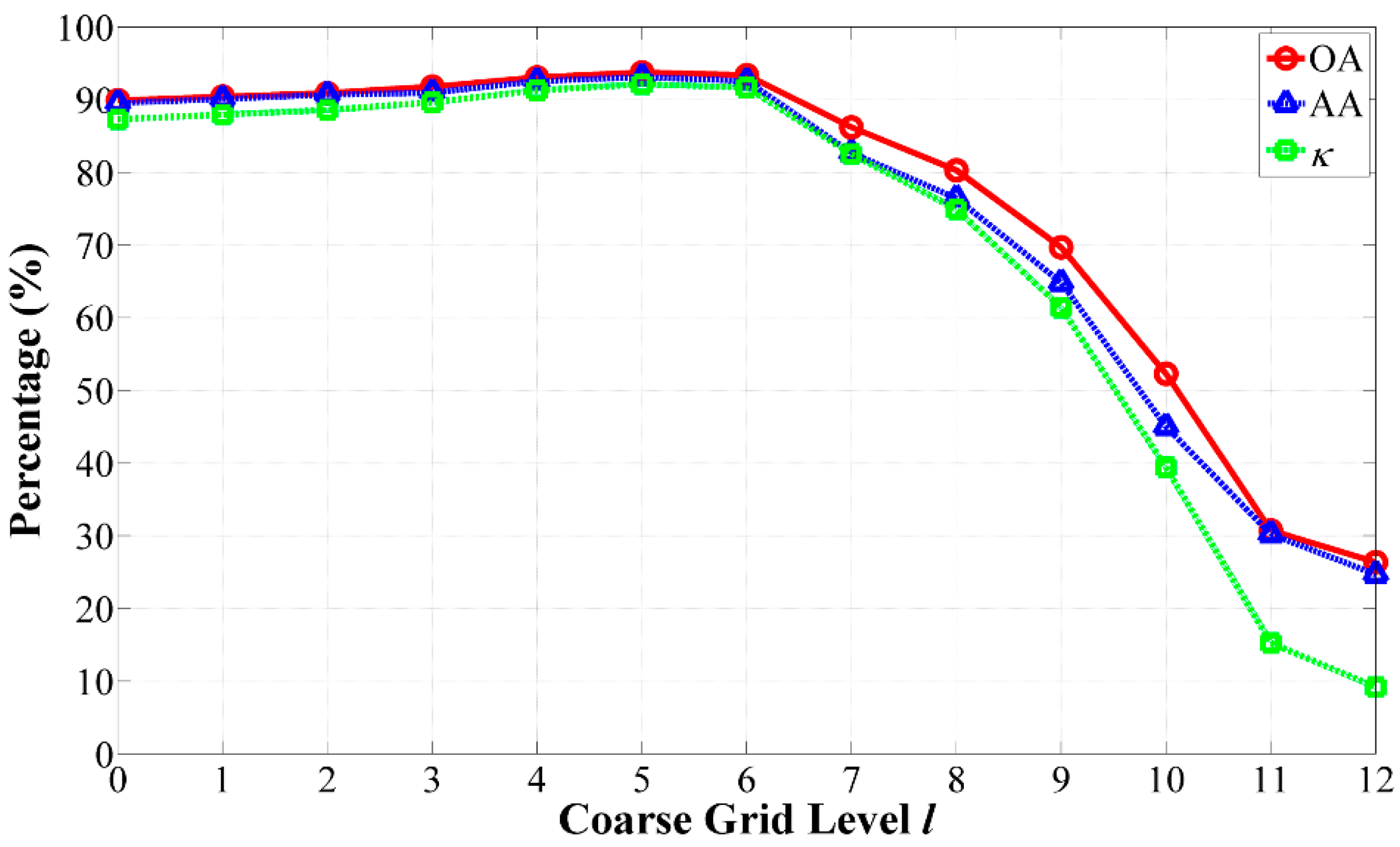
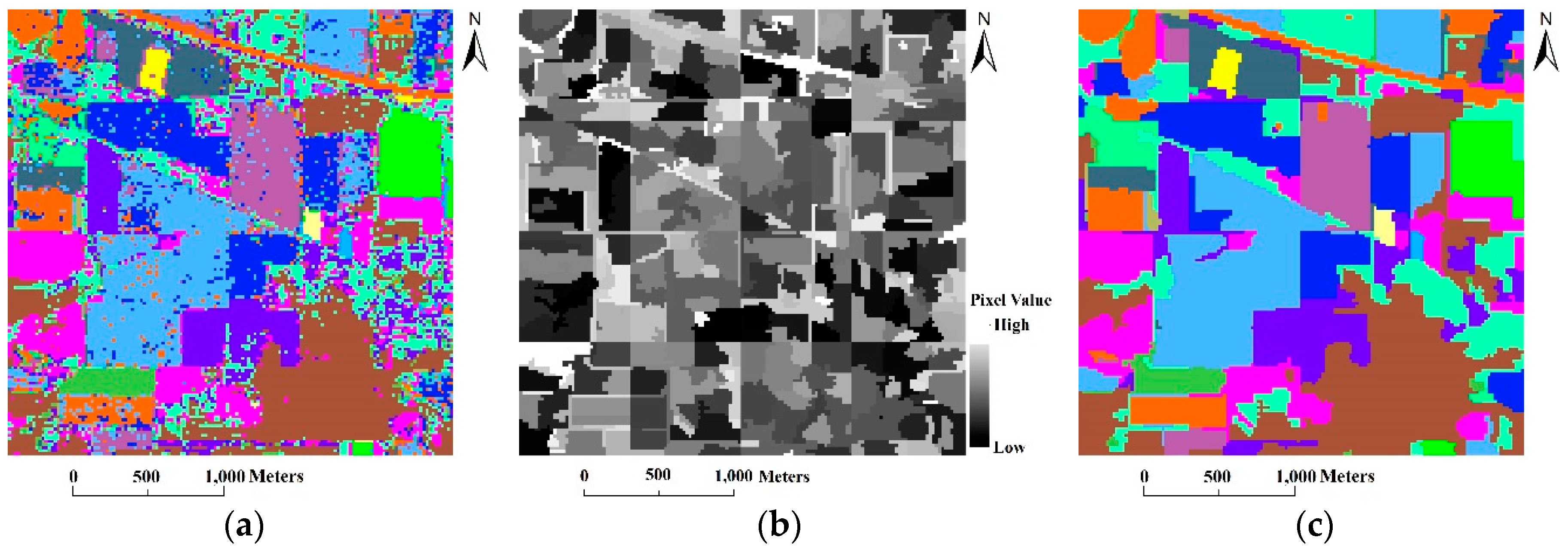
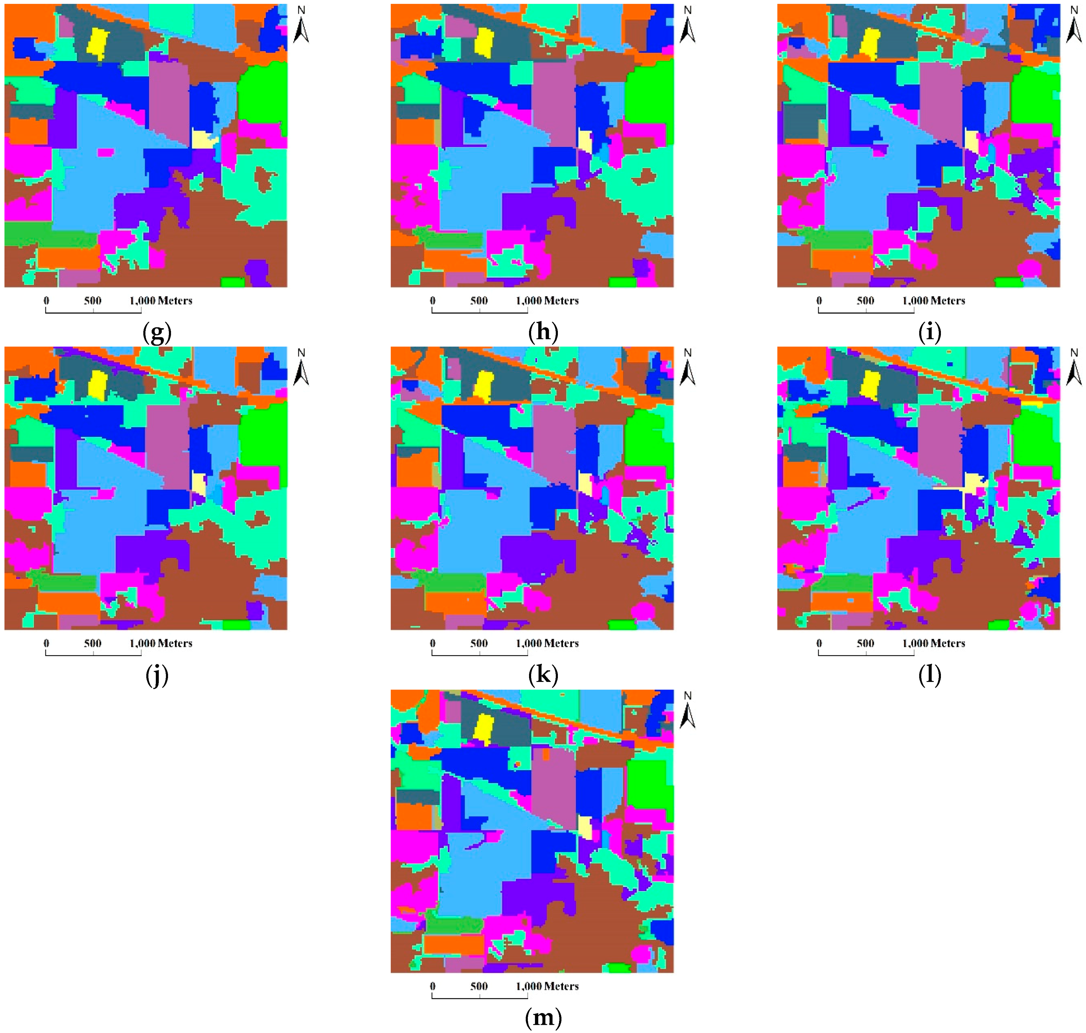
- At the coarse grid level of l = 5, our algorithm achieved the best GAs.
- (2)
- As the coarse grid level l increased, the number of regions in the HSEG maps was reduced mainly due to the decrease of the selected markers. In addition, the CAs of classes with large connected regions were improved, such as the Bldg-Grass-Tree-Drives and Oats classes (refer to the red solid line rectangles in Figure 12). On the other hand, the CAs of the classes with small connected regions were greatly reduced, such as the Grass/pasture-mowed, Soybeans-no till and Alfalfa classes (refer to the green solid line ellipses in Figure 12). It is very interesting that different values of l produced homogeneous regions with different sizes. From this point of view, the adjustability of the grid level in the multigrid structure can provide flexibility for generating different segmentation maps to satisfy various applications.
5. Conclusions
Acknowledgments
Author Contributions
Conflicts of Interest
References
- Landgrebe, D.A. Multispectral land sensing: Where from, where to? IEEE Trans. Geosci. Remote Sens. 2005, 43, 414–421. [Google Scholar] [CrossRef]
- Ham, J.; Chen, Y.; Crawford, M.M.; Ghosh, J. Investigation of the random forest framework for classification of hyperspectral data. IEEE Trans. Geosci. Remote Sens. 2005, 43, 492–501. [Google Scholar] [CrossRef]
- Samat, A.; Du, P.; Liu, S.; Cheng, L. E2lms: Emsemble extreme learning machines for hyperspectral image classification. IEEE J. Sel. Top. Appl. Earth Observ. Remote Sens. 2014, 7, 1060–1069. [Google Scholar] [CrossRef]
- Bazi, Y.; Alajlan, N.; Melgani, F.; AlHichri, H.; Malek, S.; Yager, R.R. Differential evolution extreme learning machine for the classification of hyperspectral images. IEEE Geosci. Remote Sens. Lett. 2014, 11, 1066–1070. [Google Scholar] [CrossRef]
- Mianji, F.A.; Zhang, Y. Robust hyperspectral classification using relevance vector machine. IEEE Trans. Geosci. Remote Sens. 2011, 49, 2100–2112. [Google Scholar] [CrossRef]
- Bazi, Y.; Melgani, F. Gaussian process approach to remote sensing image classification. IEEE Trans. Geosci. Remote Sens. 2010, 48, 186–197. [Google Scholar] [CrossRef]
- Sun, S.; Zhong, P.; Xiao, H.; Wang, R. Active learning with gaussian process classifier for hyperspectral image classification. IEEE Trans. Geosci. Remote Sens. 2015, 53, 1746–1760. [Google Scholar] [CrossRef]
- Camps-Valls, G.; Bruzzone, L. Kernel-based methods for hyperspectral image classification. IEEE Trans. Geosci. Remote Sens. 2005, 43, 1351–1362. [Google Scholar] [CrossRef]
- Melgani, F.; Bruzzone, L. Classification of hyperspectral remote sensing images with support vector machines. IEEE Trans. Geosci. Remote Sens. 2004, 42, 1778–1780. [Google Scholar] [CrossRef]
- Ratle, F.; Camps-Valls, G.; Weston, J. Semisupervised neural networks for efficient hyperspectral image classification. IEEE Trans. Geosci. Remote Sens. 2010, 48, 2271–2282. [Google Scholar] [CrossRef]
- Chen, Y.; Nasrabadi, N.M.; Tran, T.D. Hyperspectral image classification using dictionary-based sparse representation. IEEE Trans. Geosci. Remote Sens. 2011, 49, 3973–3985. [Google Scholar] [CrossRef]
- Yuan, H.; Tang, Y.Y.; Lu, Y.; Yang, L.; Luo, H. Hyperspectral image classification based on regularized sparse representation. IEEE J. Sel. Top. Appl. Earth Observ. Remote Sens. 2014, 7, 2174–2182. [Google Scholar] [CrossRef]
- Ma, L.; Crawford, M.M.; Yang, X.; Guo, Y. Local-manifold-learning-based graph construction for semisupervised hyperspectral image classification. IEEE Trans. Geosci. Remote Sens. 2015, 53, 2832–2844. [Google Scholar] [CrossRef]
- Huang, X.; Zhang, L. A comparative study of spatial approaches for urban mapping using hyperspectral rosis images over pavia city, northern Italy. Int. J. Remote Sens. 2009, 30, 3205–3221. [Google Scholar] [CrossRef]
- Benediktsson, J.A.; Palmason, J.A.; Sveinsson, J.R. Classification of hyperspectral data from urban areas based on extended morphological profiles. IEEE Trans. Geosci. Remote Sens. 2005, 43, 480–491. [Google Scholar] [CrossRef]
- Falco, N.; Benediktsson, J.A.; Bruzzone, L. Spectral and spatial classification of hyperspectral images based on ica and reduced morphological attribute profiles. IEEE Trans. Geosci. Remote Sens. 2015, 53, 6223–6240. [Google Scholar] [CrossRef]
- Mura, M.D.; Benediktsson, J.A.; Waske, B.; Bruzzone, L. Morphological attribute profiles for the analysis of very high resolution images. IEEE Trans. Geosci. Remote Sens. 2010, 48, 3747–3762. [Google Scholar] [CrossRef]
- Shen, L.; Zhu, Z.; Jia, S.; Zhu, J.; Sun, Y. Discriminative gabor feature selection for hyperspectral image classification. IEEE Geosci. Remote Sens. Lett. 2013, 10, 29–33. [Google Scholar] [CrossRef]
- Chen, C.; Li, W.; Su, H.; Liu, K. Spectral-spatial classification of hyperspectral image based on kernel extreme learning machine. Remote Sens. 2014, 6, 5795–5814. [Google Scholar] [CrossRef]
- Li, J.; Bioucas-Dias, J.M.; Plaza, A. Spectral-spatial hyperspectral image segmentation using subspace multinomial logistic regression and markov random fields. IEEE Trans. Geosci. Remote Sens. 2012, 50, 809–823. [Google Scholar] [CrossRef]
- Xia, J.; Chanussot, J.; Du, P.; He, X. Spectral-spatial classification for hyperspectral data using rotation forests with local feature extraction and markov random fields. IEEE Trans. Geosci. Remote Sens. 2015, 53, 2532–2546. [Google Scholar] [CrossRef]
- Camps-Valls, G.; Shervashidze, N.; Borgwardt, K.M. Spatio-spectral remote sensing image classification with graph kernels. IEEE Geosci. Remote Sens. Lett. 2010, 7, 741–745. [Google Scholar] [CrossRef]
- Li, J.; Marpu, P.R.; Plaza, A.; Bioucas-Dias, J.; Benediktsson, J.A. Generalized composite kernel framework for hyperspectral image classification. IEEE Trans. Geosci. Remote Sens. 2013, 51, 4816–4829. [Google Scholar] [CrossRef]
- Tarabalka, Y.; Tilton, J.C.; Benediktsson, J.A.; Chanussot, J. A marker-based approach for the automated selection of a single segmentation from a hierarchical set of image segmentations. IEEE J. Sel. Top. Appl. Earth Observ. Remote Sens. 2012, 5, 262–272. [Google Scholar] [CrossRef]
- Tarabalka, Y.; Chanussot, J.; Benediktsson, J.A. Segmentation and classification of hyperspectral images using minimum spanning forest grown from automatically selected markers. IEEE Trans. Syst. Man Cybern. B Cybernet. 2010, 40, 1267–1279. [Google Scholar] [CrossRef] [PubMed]
- Kimmel, R.; Yavneh, I. An algebraic multigrid approach for image analysis. SIAM J. Sci. Comput. 2003, 24, 1218–1231. [Google Scholar] [CrossRef]
- Perona, P.; Malik, J. Scale-space and edge detection using anisotropic diffusion. IEEE Trans. Pattern Anal. Mach. Intell. 1990, 12, 629–639. [Google Scholar] [CrossRef]
- Black, M.J.; Sapiro, G.; Marimont, D.H.; Heeger, D. Robust anisotropic diffusion. IEEE Trans. Image Process. 1998, 7, 421–432. [Google Scholar] [CrossRef] [PubMed]
- Mrázek, P.; Navara, M. Selection of optimal stopping time for nonlinear diffusion filtering. Int. J. Comput. Vis. 2003, 52, 189–203. [Google Scholar] [CrossRef]
- Voci, F.; Eiho, S.; Sugimoto, N.; Sekibuchi, H. Estimating the gradient in the perona-malik equation. IEEE Signal Process. Mag. 2004, 21, 39–65. [Google Scholar] [CrossRef]
- Weickert, J.; Romeny, B.M.T.H.; Viergever, M.A. Efficient and reliable schemes for nonlinear diffusion filtering. IEEE Trans. Geosci. Remote Sens. 1998, 7, 398–410. [Google Scholar] [CrossRef] [PubMed]
- Duarte-Carvajalino, J.M.; Castillo, P.E.; Velez-Reyes, M. Comparative study of semi-implicit schemes for nonlinear diffusion in hyperspectral imagery. IEEE Trans. Image Process. 2007, 16, 1303–1314. [Google Scholar] [CrossRef] [PubMed]
- Duarte-Carvajalino, J.M.; Sapiro, G.; Vélez-Reyes, M.; Castillo, P.E. Multiscale representation and segmentation of hyperspectral imagery using geometric partial differential equations and algebraic multigrid methods. IEEE Trans. Geosci. Remote Sens. 2008, 46, 2418–2434. [Google Scholar] [CrossRef]
- Briggs, W.L.; Henson, V.E.; McCormick, S.F. A Multigrid Tutorial, 2nd ed.; SIAM: Philadelphia, PA, USA, 2000; pp. 7–48. [Google Scholar]
- Tilton, J.C. RHSEG User’s Manual: Including HSWO, HSEG, HSEGExtract, HSEGReader and HSEGViewer, Version 1.50. Available online: http://opensource.gsfc.nasa.gov/projects/HSEG/RHSEG%20User's%20Manual%20V1.47.pdf (accessed on 24 March 2016).
- Mathieu, F.; Jocelyn, C.; Atli, B.J. A spatial–spectral kernel-based approach for the classification of remote-sensing images. Pattern Recognit. 2012, 45, 381–392. [Google Scholar]
- Vapnik, V.N. Statistical Learning Theory; Wiley: New York, NY, USA, 1998. [Google Scholar]
- Chang, C.-C.; Lin, C.-J. Libsvm: A library for support vector machines. ACM Trans. Intell. Syst. Technol. 2011, 2, 27. [Google Scholar] [CrossRef]
- Hsu, C.-W.; Chang, C.-C.; Lin, C.-J. A Practical Guide to Support Vector Classification; Technical Report; Department of Computer Science, National Taiwan University: Taipei, Taiwan, 2003; pp. 1–12. [Google Scholar]
- Richards, J.A.; Jia, X. Remote Sensing Digital Image Analysis: An Introduction; Springer-Verlag: New York, NY, USA, 1999. [Google Scholar]


| Class | Indiana Pines | Washington DC | Centre of Pavia | |||||||||
|---|---|---|---|---|---|---|---|---|---|---|---|---|
| Name | Training | Test | SVM | Name | Training | Test | SVM | Name | Training | Test | SVM | |
| 1 | Alfalfa | 10 | 44 | 81.82 | Grass | 52 | 1000 | 93.00 | Water | 39 | 1940 | 100 |
| 2 | Corn-no till | 143 | 1291 | 76.61 | Street | 76 | 1463 | 94.05 | Road | 80 | 3968 | 90.93 |
| 3 | Corn-min till | 83 | 751 | 72.7 | Roofs | 129 | 2468 | 88.29 | Trees | 64 | 3145 | 89.41 |
| 4 | Corn | 23 | 211 | 46.45 | Shadow | 38 | 741 | 74.63 | Grass | 54 | 2659 | 92.59 |
| 5 | Grass/pasture | 49 | 448 | 86.16 | Path | 42 | 812 | 88.67 | Soil | 67 | 3293 | 98.45 |
| 6 | Grass/trees | 74 | 673 | 89.75 | Trees | 44 | 840 | 98.57 | Bricks | 40 | 1984 | 90.57 |
| 7 | Grass/pasture-mowed | 10 | 16 | 87.50 | Bitumen | 49 | 2421 | 88.76 | ||||
| 8 | Hay-windrowed | 48 | 441 | 97.28 | Shadow | 30 | 1503 | 95.94 | ||||
| 9 | Oats | 10 | 10 | 100 | Roof-1 | 39 | 1959 | 93.72 | ||||
| 10 | Soybeans-no till | 96 | 872 | 83.03 | Roof-2 | 77 | 3817 | 74.33 | ||||
| 11 | Soybeans-min till | 246 | 2222 | 87.62 | ||||||||
| 12 | Soybeans-clean till | 61 | 553 | 66.55 | ||||||||
| 13 | Wheat | 21 | 191 | 96.34 | ||||||||
| 14 | Woods | 129 | 1165 | 93.30 | ||||||||
| 15 | Bldg-Grass-Trees-Drives | 38 | 342 | 61.40 | ||||||||
| 16 | Stone-steel towers | 10 | 85 | 63.53 | ||||||||
| Total | 1051 | 9315 | Total | 381 | 7324 | Total | 539 | 26,689 | ||||
| OA | 82.51 | OA | 89.92 | OA | 90.39 | |||||||
| AA | 80.63 | AA | 89.54 | AA | 91.47 | |||||||
| 79.96 | 87.31 | 89.23 | ||||||||||
| AMG-M-HSEG | Proba-M-HSEG | Proba-M-HSEG + MV | Morph-M-HSEG | Morph-M-HSEG + MV | Proba-M-MSF | Proba-M-MSF + MV | ||||
|---|---|---|---|---|---|---|---|---|---|---|
| DC | ED | SAM | SAM | SAM | SAM | SAM | ED | SAM | ED | SAM |
| OA | 95.16 | 96.32 | 94.49 | 94.86 | 95.04 | 95.04 | 93.17 | 91.44 | 93.33 | 94.04 |
| AA | 95.21 | 95.97 | 93.16 | 93.35 | 86.88 | 86.88 | 92.95 | 91.46 | 86.26 | 93.91 |
| 94.48 | 95.80 | 93.71 | 94.13 | 94.33 | 94.33 | 92.21 | 90.24 | 92.37 | 93.20 | |
| Alfalfa | 86.36 | 86.36 | 86.36 | 86.36 | 86.36 | 86.36 | 88.64 | 88.64 | 88.64 | 88.64 |
| Corn-no till | 92.10 | 92.33 | 87.06 | 87.06 | 86.91 | 86.91 | 94.42 | 87.61 | 87.76 | 87.61 |
| Corn-min till | 93.74 | 96.67 | 92.81 | 95.07 | 97.74 | 97.74 | 82.96 | 77.23 | 94.54 | 94.67 |
| Corn | 91.47 | 99.33 | 82.46 | 82.46 | 79.15 | 79.15 | 79.15 | 97.16 | 79.15 | 97.16 |
| Grass/pasture | 95.76 | 96.43 | 94.64 | 94.64 | 93.75 | 93.75 | 93.75 | 93.75 | 92.41 | 93.75 |
| Grass/trees | 97.18 | 96.43 | 95.99 | 95.99 | 98.07 | 98.07 | 96.88 | 92.27 | 96.88 | 96.43 |
| Grass/pasture-mowed | 93.75 | 93.75 | 93.75 | 93.75 | 75.00 | 75.00 | 93.75 | 93.75 | 93.75 | 93.75 |
| Hay-windrowed | 99.55 | 93.42 | 99.77 | 99.77 | 99.77 | 99.77 | 99.77 | 99.55 | 99.55 | 97.51 |
| Oats | 100 | 100 | 90.00 | 90.00 | 0 | 0 | 100 | 100 | 0 | 100 |
| Soybeans-no till | 85.44 | 91.97 | 88.76 | 88.76 | 89.33 | 89.33 | 91.86 | 91.06 | 85.21 | 90.25 |
| Soybeans-min till | 96.22 | 98.51 | 98.92 | 99.68 | 99.01 | 99.01 | 93.43 | 94.82 | 98.47 | 97.70 |
| Soybeans-clean till | 98.73 | 95.3 | 97.29 | 97.29 | 97.11 | 97.11 | 86.44 | 97.29 | 90.78 | 85.35 |
| Wheat | 100 | 98.95 | 99.48 | 99.48 | 99.48 | 99.48 | 99.48 | 100 | 99.48 | 100 |
| Woods | 99.48 | 98.88 | 99.66 | 99.66 | 99.83 | 99.83 | 99.57 | 100 | 99.31 | 100 |
| Bldg-Grass-Tree-Drives | 97.08 | 98.83 | 84.80 | 84.80 | 89.77 | 89.77 | 89.47 | 52.63 | 76.61 | 82.16 |
| Stone-steel towers | 96.47 | 97.65 | 98.82 | 98.82 | 98.82 | 98.82 | 97.65 | 97.65 | 97.65 | 97.65 |
| AMG-M-HSEG | Proba-M-HSEG | Proba-M-HSEG + MV | Morph-M-HSEG | Morph-M-HSEG + MV | Proba-M-MSF | Proba-M-MSF + MV | ||||
|---|---|---|---|---|---|---|---|---|---|---|
| DC | ED | SAM | SAM | SAM | SAM | SAM | ED | SAM | ED | SAM |
| OA | 92.80 | 93.76 | 90.36 | 91.79 | 92.91 | 92.93 | 85.89 | 84.18 | 91.08 | 92.69 |
| AA | 92.80 | 93.12 | 91.05 | 91.75 | 92.48 | 92.49 | 87.41 | 86.44 | 90.45 | 91.75 |
| 90.95 | 92.14 | 87.92 | 89.69 | 91.08 | 91.10 | 82.42 | 80.39 | 88.79 | 90.80 | |
| Grass | 94.20 | 94.5 | 94.90 | 95.20 | 95.30 | 95.30 | 96.10 | 95.30 | 96.7 | 95.30 |
| Street | 97.88 | 97.88 | 97.33 | 97.33 | 98.29 | 98.29 | 86.67 | 82.09 | 98.22 | 98.22 |
| Roofs | 91.73 | 93.40 | 84.68 | 88.86 | 91.33 | 91.37 | 79.94 | 77.07 | 88.90 | 92.26 |
| Shadow | 81.78 | 83.40 | 84.48 | 82.32 | 84.08 | 84.08 | 89.2 | 86.77 | 80.43 | 77.73 |
| Path | 88.30 | 90.39 | 86.58 | 88.42 | 87.19 | 87.19 | 75.62 | 87.68 | 78.69 | 87.59 |
| Trees | 99.52 | 99.17 | 98.33 | 98.33 | 98.69 | 98.69 | 96.9 | 89.76 | 99.76 | 99.40 |
| AMG-M-HSEG | Proba-M-HSEG | Proba-M-HSEG + MV | Morph-M-HSEG | Morph-M-HSEG + MV | Proba-M-MSF | Proba-M-MSF + MV | ||||
|---|---|---|---|---|---|---|---|---|---|---|
| DC | ED | SAM | SAM | SAM | SAM | SAM | ED | SAM | ED | SAM |
| OA | 96.06 | 97.45 | 95.32 | 95.64 | 95.32 | 95.64 | 90.98 | 87.14 | 95.29 | 92.74 |
| AA | 96.58 | 97.43 | 95.42 | 95.92 | 95.42 | 95.92 | 90.38 | 83.88 | 95.87 | 92.63 |
| 95.58 | 97.14 | 94.74 | 95.1 | 94.74 | 95.1 | 89.87 | 85.49 | 94.2 | 91.86 | |
| Water | 99.85 | 100 | 100 | 100 | 100 | 100 | 100 | 100 | 99.18 | 99.85 |
| Road | 95.79 | 98.36 | 93.37 | 92.67 | 93.37 | 92.67 | 97.43 | 91.94 | 91.68 | 87.15 |
| Trees | 93 | 98.12 | 93.83 | 89.35 | 93.83 | 89.35 | 74.15 | 84.61 | 85.79 | 89.57 |
| Grass | 98.5 | 96.8 | 85.41 | 93.23 | 85.41 | 93.23 | 99.14 | 78.9 | 98.91 | 89.51 |
| Soil | 99.97 | 100 | 100 | 100 | 100 | 100 | 99.94 | 100 | 99.79 | 100 |
| Bricks | 97.53 | 96.88 | 97.23 | 99.5 | 97.23 | 99.5 | 81.85 | 94.71 | 95.21 | 98.44 |
| Bitumen | 95.95 | 93.27 | 96.61 | 96.28 | 96.61 | 96.28 | 90.62 | 96.86 | 95.46 | 94.96 |
| Shadow | 99.07 | 96.14 | 92.88 | 93.15 | 92.88 | 93.15 | 99.07 | 27.15 | 98.27 | 74.52 |
| Roof-1 | 96.32 | 99.29 | 98.11 | 98.11 | 98.11 | 98.11 | 67.79 | 70.04 | 99.08 | 99.29 |
| Roof-2 | 89.83 | 95.44 | 96.75 | 96.91 | 96.75 | 96.91 | 93.82 | 94.63 | 95.34 | 93 |
| Class | l = 4 | l = 5 | l = 6 |
|---|---|---|---|
| OA | 95.35 | 96.32 | 95.81 |
| AA | 94.59 | 95.97 | 88.99 |
| 94.70 | 95.80 | 95.22 | |
| Alfalfa | 86.36 | 86.36 | 70.45 |
| Corn-no till | 87.14 | 92.33 | 91.94 |
| Corn-min till | 93.74 | 96.67 | 96.94 |
| Corn | 96.21 | 99.33 | 97.63 |
| Grass/pasture | 98.21 | 96.43 | 93.08 |
| Grass/trees | 97.77 | 96.43 | 97.62 |
| Grass/pasture-mowed | 93.75 | 93.75 | 0 |
| Hay-windrowed | 99.77 | 93.42 | 99.77 |
| Oats | 80.00 | 100 | 100 |
| Soybeans-no till | 91.17 | 91.97 | 85.44 |
| Soybeans-min till | 96.98 | 98.51 | 99.01 |
| Soybeans-clean till | 97.65 | 95.30 | 96.93 |
| Wheat | 100 | 98.95 | 99.48 |
| Woods | 98.80 | 98.88 | 96.93 |
| Bldg-Grass-Tree-Drives | 98.25 | 98.83 | 99.48 |
| Stone-steel towers | 97.65 | 97.65 | 99.40 |
© 2016 by the authors; licensee MDPI, Basel, Switzerland. This article is an open access article distributed under the terms and conditions of the Creative Commons by Attribution (CC-BY) license (http://creativecommons.org/licenses/by/4.0/).
Share and Cite
Song, H.; Wang, Y. A Spectral-Spatial Classification of Hyperspectral Images Based on the Algebraic Multigrid Method and Hierarchical Segmentation Algorithm. Remote Sens. 2016, 8, 296. https://doi.org/10.3390/rs8040296
Song H, Wang Y. A Spectral-Spatial Classification of Hyperspectral Images Based on the Algebraic Multigrid Method and Hierarchical Segmentation Algorithm. Remote Sensing. 2016; 8(4):296. https://doi.org/10.3390/rs8040296
Chicago/Turabian StyleSong, Haiwei, and Yi Wang. 2016. "A Spectral-Spatial Classification of Hyperspectral Images Based on the Algebraic Multigrid Method and Hierarchical Segmentation Algorithm" Remote Sensing 8, no. 4: 296. https://doi.org/10.3390/rs8040296
APA StyleSong, H., & Wang, Y. (2016). A Spectral-Spatial Classification of Hyperspectral Images Based on the Algebraic Multigrid Method and Hierarchical Segmentation Algorithm. Remote Sensing, 8(4), 296. https://doi.org/10.3390/rs8040296