Article

Registration of Long-Strip Terrestrial Laser Scanning Point Clouds Using RANSAC and Closed Constraint Adjustment

1
School of Geodesy and Geomatics, Wuhan University, Wuhan 430079, China
2
Department of Geography and GeoInformation Sciences, College of Science, George Mason University, Fairfax, VA 22030, USA
3
School of Remote Sensing and Information Engineering, Wuhan University, Wuhan 430079, China
4
Department of Geography & Environmental Management, University of Waterloo, ON N2L3G1, Canada
*
Author to whom correspondence should be addressed.
Remote Sens. 2016, 8(4), 278; https://doi.org/10.3390/rs8040278
Submission received: 30 December 2015 / Revised: 10 March 2016 / Accepted: 21 March 2016 / Published: 28 March 2016

Abstract

:
The registration of long-strip, terrestrial laser scanning (TLS) point clouds is a prerequisite for various engineering tasks, including tunnels, bridges, and roads. An artificial target-based registration method is proposed in this paper to automatically calculate registration parameters (i.e., rotation, translation) of scanned pairs without initial estimations. The approach is based on the well-known Random Sample Consensus (RANSAC) method and effectively searches the point cloud for corresponding returns from a system of artificial targets. In addition, Closed Constraint Adjustment (CCA) is integrated into the registration method to significantly reduce the accumulative error. Experimental results demonstrate the robustness and feasibility of the proposed approach. It is a promising approach to register automatically long strips with limited external control points with satisfactory precision.

Graphical Abstract

1. Introduction

The strong urbanization trends of the past few decades are leading to even more complex construction environments, thus raising the demand for dense and accurate three-dimensional (3D) data. For example, the substantial air pollution problems encountered in the world’s megacities [1] force countries like China to consider alternative solutions to automobile-based transportation. High-speed rail is thus becoming a very attractive option, especially when considered against a backdrop of worsening airport congestion and given its reduced carbon footprint. However, in order to pursue this option we are faced with substantial engineering challenges. Viewed as 3D objects, high-speed rails and their ancillary infrastructure (e.g., tunnels, bridges, and piers) are complex, challenging, and labor-intensive for traditional surveying solutions (e.g., leveling or triangulation). It is becoming even more challenging if one considers the need to regularly monitor these complex structures.
Laser scanning technology offers a quick and low-cost alternative for the acquisition of large amounts of 3D information. In terrestrial applications, laser scanning allows the collection of detailed façade information with high geometric precision. Terrestrial laser scanning (TLS) is a ground-based, active imaging method that rapidly acquires accurate, dense 3D point clouds of object surfaces through laser range finding. The number and variety of applications that benefit from TLS continue to increase, including landscape measurements, measuring and modeling for complex industrial equipment, building and heritage conservation, 3D urban visualization modeling, surveys for forest and agricultural resources, and deformation monitoring [2,3,4,5].
When applied to elongated features such as high-speed rails, TLS presents challenges as such applications require numerous long-strip scans to complete a scene. The point cloud sets acquired by such successive scans are referenced to different local frames, each associated with a corresponding scanner location. Therefore, a registration process is needed to align and merge these individual scans relative to a common reference frame. This registration results in the generation of long 3D strips, like the long geolocated 2D mosaics derived through image co-registration [6]. The co-registration of individual point cloud scenes is a prototypical photogrammetric problem, comparable to traditional strip adjustments, and requiring the estimation of transformation parameters describing the relative position of two overlapping 3D models, namely the scale, shifts, and rotation of one 3D scene relative to another. This is the subject of this publication.
The registered TLS data are the final measurement product and are in the form of a point cloud, consisting of a set of data points defined by their X, Y, and Z coordinates. However, these final measurement products are normally distorted due to registration errors and these errors are accumulated in multi-site cloud registration, especially in surveyed areas with limited control points. The resulting compromised accuracy not only affects the reliability but also restricts the applications of TLS data. Overall, the accuracy of the acquired TLS data is affected by two primary aspects: ranging accuracy of the scanner, and registration accuracy among multiple point cloud data [7,8]. As a simple and robust method for finding a set of inliers, the popular RANdom Sample Consensus (RANSAC) algorithm (Fischler and Bolles [9]), can be used to register point clouds. However, the accuracy of RANSAC is affected by determining the assumed noise in the surface direction, a function of the distance from an object to the laser scanner, incident angle, surface texture, and point clouds generated by multiple scan setups. In order to improve the overall accuracy, we propose a RANSAC-based registration that is enhanced through a Closed Constraint Adjustment (CCA). This Closed Constraint Adjustment (CCA) ensures that loops are closed. In the context of this publication we consider as representative objects to be measured the types of bridge piers that are used as basic docks for high speed rail (HSR).
This paper is organized as follows. Section 2 reviews different registration techniques. Section 3 describes the proposed registration methods based on the introduction of the registration method using artificial targets and the basic principles of Random sample consensus (RANSAC). Section 4 discusses the experimental results of the proposed registration methods, followed by Section 5 with conclusions and recommendations for further research.

2. Literature Review

Several approaches have emerged for the co-registration of laser scans, with each of them distinguished by its particular target functions and objectives. For example, the Iterative Closest Point (ICP) algorithm is based on minimizing the point-to-point distance in the overlapping area between different TLS scans [10]. Popular variations of ICP include the Iterative Closest Patch (ICPatch) [11] and the Iterative Closest Projected Point (ICPP) [12]. Commonly, ICP-based methods require large overlap among the data sets and accurate initial approximations of the transformation parameters. However, even if there is considerable overlap, convergence to a global minimum is not guaranteed. Furthermore, ICP-based methods are computationally intensive and time consuming in their search for conjugate points in overlapping scans using all available points [13]. As an improvement, Bae and Lichti [14] proposed a robust automated registration method for unorganized point clouds, namely the Geometric Primitive ICP with RANSAC (GP-ICPR). In that approach, a modified RANSAC algorithm is used for outlier removal. All the possible point-pair matches are used to estimate the transformation parameters between the two data sets.
Another commonly used algorithm (Chen and Medioni [15]), minimizes the point-to-plane distance in the overlapping area of the TLS scans. It also requires a very good initial alignment to eventually produce a successful solution. This algorithm is generally faster than ICP. However, the point clouds need to be initially more closely aligned to each other compared to the requirements of ICP. ICP, its variants, and Chen and Medioni’s algorithm assume that the closest point in a point cloud is a good estimate of the correct corresponding point. If two point clouds are not approximately aligned using available georeferencing information, this assumption is not necessarily correct. Although initial alignment can be provided by other means (e.g., surveying of the laser scanner locations), this option is not always possible. Although these adjustment algorithms provide a closed-form solution (i.e., no iteration), one of the reasons for their popularity, these methods cannot provide statistical information of individual parameters of rigid body transformation as conventional least square methods can offer.
Recent efforts have produced approaches that use not only points, but also lines and surfaces as registration primitives [16,17,18]. Various geometric primitives (e.g., planes, lines, spheres) are derived from point clouds and are subsequently used to register TLS scans instead of using all available points. For instance, Rabbani et al. [19] registered scans of an industrial site rich in different geometric features by extracting and comparing the site’s features. Using lines as major geometric primitives, Eo et al. [20] showed that line-based matching may give better results than point-based matching. The results of Sibel Canaz [21] indicate that a linear feature-based registration method is more flexible than a planar feature-based registration method. Line features represent geometric evidence of edges, which are quite prominent and extraordinary, and thus matching conjugate line features may produce more robust and reliable results. Nevertheless, due to issues such as completeness and precision of these extracted line features, their direct matching is not trivial. Plane features have also been used for registration. Brenner et al. [22] showed that three plane matches can help determine the transformation parameters between two point clouds, and their method was later compared with the point-based Normal Distributions Transform method. The combination of different primitives has also been studied. Jaw and Chuang [23] used point-based, line-based, and planar-based registration techniques, both individually and collectively and demonstrated that their combination produced more reliable registration results than single features. Similarly, Huang et al. [24] presented a method utilizing multiple geometric features for the registration of TLS data. Conjugate planes were used to find the rotation, and the intersections of the axes of the cylinders and planes were used to determine the translation. Although the comprehensive use of multi-features potentially improves the reliability and precision of registration, these algorithms require that such features are discernible in registered point clouds, which cannot always be assumed to be the case. Aiming to improve accuracy, Cheng [25] proposed and tested a model of multiple registration error propagation, without introducing a method to eliminate the accumulated error. Xu [26] assigned error for all scanning positions using the final cumulative registration errors, but the method cannot be considered as a real adjustment [26].
Therefore, despite these prior efforts, we are still lacking an algorithm that facilitates registration with high accuracy, reliability and robustness. Towards this goal, a registration method is proposed herein that uses a random sample consensus (RANSAC) for adjacent scanning positions. RANSAC is an iterative method to estimate parameters of a mathematical model from a set of observed data that contain outliers. It is a non-deterministic algorithm in that it produces a reasonable result only with a certain probability. The advantage of RANSAC is that it allows a robust estimation of the model parameters estimating the parameters with a high degree of accuracy even when a significant number of outliers are present in the data set. Long-strip, terrestrial laser scanning point clouds are registered by the target points, which are detected by RANSAC without requiring precise initial approximations. While RANSAC solves the correspondence problem and ensures correct matches it cannot ensure by itself an acceptable overall accuracy. Due to the particular nature of long-strip adjustments, errors are easily accumulated along the strip, a problem common in traditional photogrammetric strip adjustments [27]. Through the use of target points and the relationship among adjacent scanning positions one can maintain the overall stability of the solution. This joint use of RANSAC for targets correspondence, and of CCA can offer a reliable and robust solution of the co-registration problem, eliminating misclosures caused by registration errors and ensuring the reliability of the overall registration results. Table 1 shows the difference of these methods generally.
An approach comparable to this was offered by Ji et al. [28]. The difference between this paper and that of Ji et al. [28] is threefold. First, the objectives of the two papers differ. Ji et al. [28] discuss the investigation of fine registration and compare the impact of different registration methods on the overall precision of the registration process. Conversely, this paper is focused on the complete procedure of registration from target correspondence to fine registration with closing condition. Second, Ji et al. [28] propose a registration method without using a control network, which affords a complete control with sufficient control points. Ji et al. [28] set a limited number of control points but the number is insufficient for a control network to form an overall constraint. After all, the method used in Ji et al. [28] is without a control network. However, this paper utilizes the adjacency of scanning positions, visibility of control points from different scanning positions, and closing condition formed by local scanning positions to conduct an overall adjustment without control points. The results are an improvement in the precision of joint with reduced distortion, thus addressing the long strip registration challenge to a certain extent. Third, this paper further extends Ji et al. [28] by integrating in the approach the use of RANSAC for the automatic identification of correspondences. RANSAC is robust in terms of gross errors but only handles the correspondence problem without guaranteeing the overall precision. Due to the characteristics of long-strip, it is easy to accumulate error and create a distorted result. In this paper, the promise of precision is supported by the adjacency of scanning positions, visibility of target points from different scanning positions, and closing condition formed by local scanning positions. Therefore, the approach presented in this paper offers the potential of both high robustness and precision of the overall automatic long-strip registration.

3. Methodology

The proposed approach comprises two steps: (1) Point cloud registration using a robust RANSAC-based method to determine the correspondence relationship of the scanning target in two different sets of point clouds; and (2) Closed Constraint Adjustment (CCA) to eliminate the accumulated registration errors for point cloud data of all scanning positions.

3.1. RANSAC Algorithm

The correspondence relation of a scanning target in two different sets of point clouds is determined by the local description of the target’s salient features. However, the ambiguity of local description may result in incorrect correspondences. To avoid the inaccuracy, existing robust methods check the consistency of the data against a global model and discard spurious data. Among the robust methods, the RANSAC is one of the most successful and widely used, especially in the Computer Vision community, and was first published by Fischler and Bolles in 1981 [9].
RANSAC iteratively estimates parameters of a mathematical model from a set of observed data containing outliers. It produces reasonable results with a certain probability, and the probability increases with increasing iterations. One of the most well-known applications of RANSAC is to solve the Location Determination Problem (LDP) [9]. A basic assumption of RANSAC is that the data consists of “inliers” and “outliers”. Inliers are referred to as data whose distribution is explained by a set of model parameters, whereas outliers are data that do not fit the model. Outliers originate from extreme values of the noise, erroneous measurements, or incorrect hypotheses about the interpretation of the data. The RANSAC assumes that there exists a procedure to estimate the parameters of a model to optimally explain or fit the data, given a (usually small) set of inliers.
The RANSAC algorithm initially selects a random subset of the observed data points, and using this subset, a fitting model is computed. All other data are tested using this fitted model, and points that fit the estimated model are a consensus set, whereas points that do not fit the estimated model are considered outliers. RANSAC iteratively repeats the above steps until a sufficient number of points are classified as part of the consensus set. An advantage of RANSAC is its ability to conduct robust estimation [9] of the model parameters, even in the presence of a large number of outliers. A disadvantage of RANSAC is that no upper bound exists for the computational time to estimate these parameters. When the number of iterations is limited, the solution may not be optimal and may not be one that fits the data satisfactorily. Thus, RANSAC offers a trade-off by computing a greater number of iterations, the probability of a reasonable model being produced increases. Moreover, RANSAC does not always find the optimal set, even for moderately contaminated sets, and usually has a less-than-optimal performance when the number of inliers is <50%. Optimal RANSAC [29] is designed to address these problems and is capable of finding the optimal set for heavily contaminated sets, even for an inlier ratio <5%.
Another disadvantage of RANSAC is the requirement of problem-specific thresholds. RANSAC only estimates one model for a particular data set. As for any one-model approach when two (or more) model instances exist, RANSAC fails to find either outcome. The Hough [30] transform is an alternative robust estimation technique that may be useful when there is more than one model instance. Another approach for multi-model fitting is PEARL [31], which combines model sampling from data points as in RANSAC with iterative re-estimation of inliers and the multi-model fitting formulated as an optimization problem with a global energy function describing the quality of the overall solution.

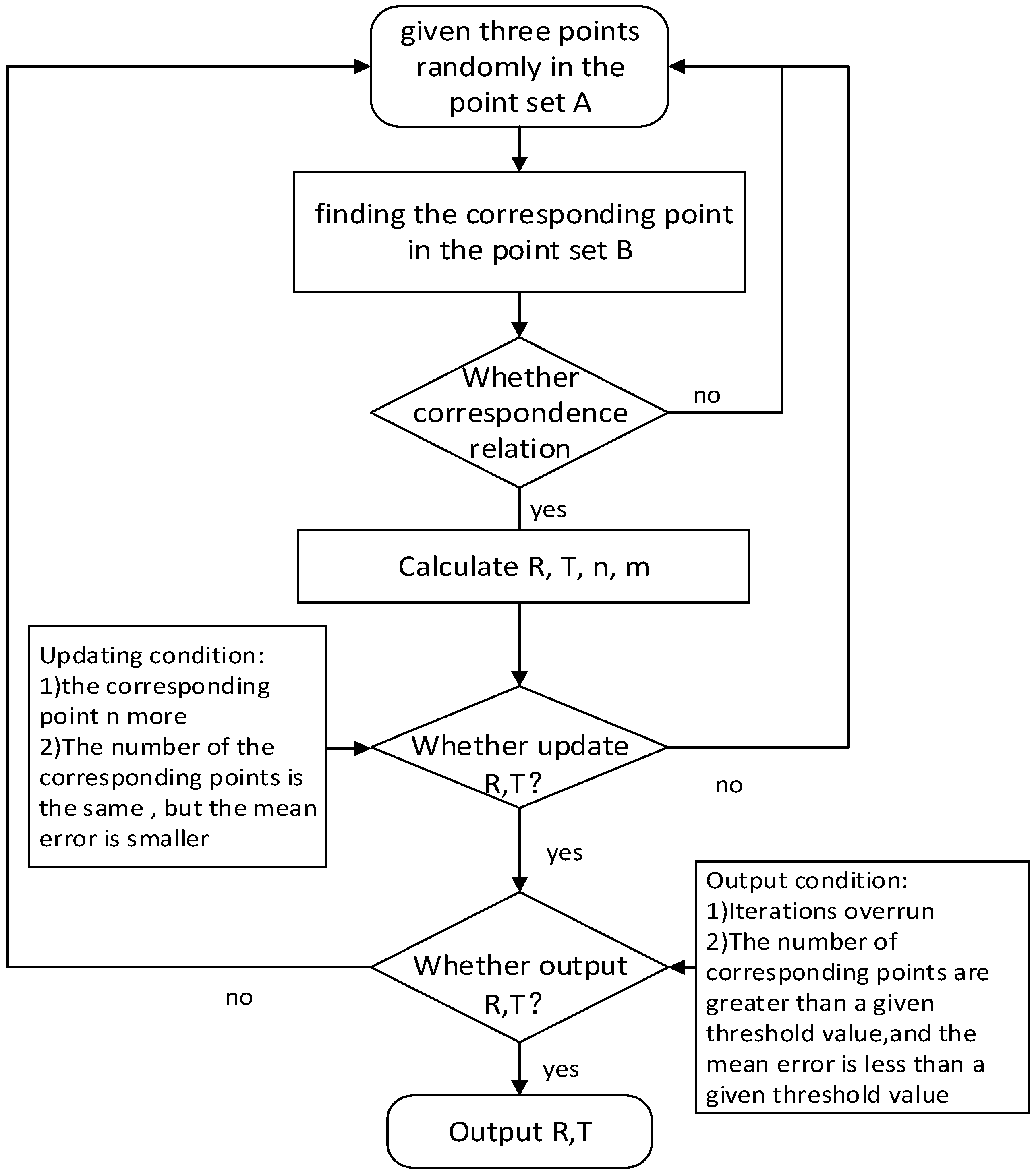
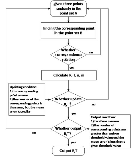
3.2. RANSAC-Based Registration of TLS Data

In this section, we introduce the methodology for RANSAC-based registration of terrestrial laser scans. The methodology is based on determining the correspondence relation of the scanning target in two different sets of point clouds. After acquiring data by a terrestrial three-dimensional scanner, the coordinates of the scanning target are extracted, and the correspondence relation of two targets is identified from two different sets of targets by the RANSAC algorithm to achieve cloud registration from the two-site point clouds.
The relative position invariance in space of the two targets is essential to identify their correspondence relation using RANSAC. This principle is illustrated in Figure 1.
(1)
Given two point sets A and B , randomly select three points a 1 , a 2 , a 3 A and similarly select three points in the point set B. First, calculate the mode of the vector a 1 a 2 and the vector b 1 b 2 ( b 1 , b 2 B ) , with the constraints of a 1 a 2 b 1 b 2 < t h r e s h o l d 1 .
(2)
Find the correspondence relations a 1 a 3 , a 2 a 3 from the point set vector B in the same way. If the correspondence in the three groups is exactly three points b 1 , b 2 , b 3 in the point set B , the relationship of the point set A 1 ( a 1 , a 2 , a 3 ) and point set B 1 ( b 1 , b 2 , b 3 ) is:.
R 0 a n + T 0 = b n ( n 0 , 1 , 2 )
[ r ( 0 , 0 ) r ( 0 , 1 ) r ( 0 , 2 ) r ( 1 , 0 ) r ( 1 , 1 ) r ( 1 , 2 ) r ( 2 , 0 ) r ( 2 , 1 ) r ( 2 , 2 ) ] [ a 1 a 2 a 3 ] + [ t x t y t z ] = [ b 1 b 2 b 3 ]
where R and T the corresponding rotation matrix and translation vector.
(3)
Calculate R, T, n, and m according to Equations (1) and (2). The initial value R 0 , T 0 of the rotation and translation between the two scanning positions is obtained through these equations, and the resulting the residual vector of the points V = ( v x , v y , v z ) is calculated using through Equation (3). In Equation (3), ( x a n , y a n , z a n ) and ( x b n , y b n , z b n ) are the conjugate coordinates in the scanning positions a n and b n , respectively. In addition, the mean error of the registration for the two scanning positions is obtained from Equation (4).
[ r ( 0 , 0 ) r ( 0 , 1 ) r ( 0 , 2 ) r ( 1 , 0 ) r ( 1 , 1 ) r ( 1 , 2 ) r ( 2 , 0 ) r ( 2 , 1 ) r ( 2 , 2 ) ] [ x a n y a n z a n ] + [ t 0 t 1 t 2 ] [ x b n y b n z b n ] = [ v x v y v z ]
m 0 = V 1 2 + V 2 2 + ... + V n 2 n
Using the above matrix initial value R 0 , V 0 , mapping C in the point set B coordinate system from all points in the point set B is calculated. Consequently, the nearest point b n from each point c n in the point set C is computed. If b n c n ¯ < t h r e s h o l d 2 , then ( a n , b n ) is a set of corresponding points, and a n is c n ’ s corresponding point in the point set A. After finding all corresponding points, the point sets A 1 ( a 1 , a 2 , ... , a n ) , B 1 ( b 1 , b 2 , ... , b n ) are updated, and a new rotation matrix R 1 and T 1 is obtained.
(4)
Iterations follow in order to refine the solution as needed. The above steps are repeated, and the matrices R and T are updated if one of the following two conditions is met in the k t h iteration:
(i)
The number of corresponding points in the point set A 1 , B 1 : n k > n k 1 or
(ii)
The number of the corresponding points in the point set A 1 , B 1 : n k = n k 1 , and residuals m k < m k 1 .
(5)
A convergence is achieved and R and T are estimated in a typical adjustment fashion when the number of the conjugate points is > the threshold and the mean error of registration is < the threshold.
The above thresholds are calculated based on the point distance and registration requirements, (e.g., requiring registration accuracy normally below 1 cm). The experience threshold can be three times of the precision for RANSAC (3 cm).

3.3. Closed Constraint Adjustment (CCA) Based Registration for Point Cloud Data

Then RANSAC-based registration finds the conjugate (corresponding) points of the targets between two adjacent scans for calculating their transformation model parameters (R, T). There is a degree of distortion by RANSAC-based registration for adjacent scanning positions, and it requires redundant targets as a constraint condition to control the overall fit and reduce distortions. It uses the target points in the four scanning positions between the two piers and takes 1→2→3→4→1 as a closing condition to register. The shape of distribution of scanning position is like a small ring and interlocked like a chain. By the closing condition adjustment, it significantly reduces the accumulated error and obtains the most accurate results.

3.3.1. Sources of Error Analysis

Along with the scanning process, errors of the scanning coordinates may exist and affect the registration precision and accuracy. Point cloud registration is accomplished by utilizing spatial position invariance of the targets. The procedure includes two steps: (1) scanning targets from different angles and obtaining the target coordinates in the different scanning coordinate systems; and (2) using rigid body transformation by the coordinate information to complete the registration. Several factors affect the accuracy of this approach:
(1)
Range accuracy of a three-dimensional scanner is limited;
(2)
Scanning in different angles generates errors due to different incident angles;
(3)
Extraction accuracy for the center of the target is affected, as the target has strong reflection and will be "floated" from the background objects; and
(4)
External environmental factors, including atmospheric conditions and scattered light, might affect the working status of the scanner and the reflection of the target.

3.3.2. Propagation of Registration Error

The mathematical model of the point cloud registration by the targets is a basic 3D projection model and is expressed in Equation (5):
f = [ X B Y B Z B ] = [ cos y cos p sin y cos r + cos y sin p sin r sin y sin r + cos y sin p cos r sin y cos p      cos y cos r + sin y sin p sin y sin r sin y + sin y sin p cos r sin p          cos p sin r          cos p cos r ] [ X A Y A Z A ] + [ t x t y t z ]
where ( X A , Y A , Z A ) and ( X B , Y B , Z B ) are coordinates in the respective scanning data for the same target, ( y , p ,    r ) are the three rotation angles around the coordinate axes, and ( t x , t y , t z ) is the corresponding translation vector. This is abbreviated in standard least squares notation as B = R A + T , where A , B are the model’s coordinates, R is the rotation matrix, and T is the translation vector. An indirect adjustment model is created by selecting ( y , p , r , t x , t y , t z ) as an independent value. In accordance with the principle of non-linear adjustment model, the above non-linear equations are processed differently. The equations are obtained in Equation (6):
[ V x V y V z ] = [ f x p f x y f x r f x t x f x t y f x t z f y p f y y f y r f y t x f y t y f y t z f z p f z y f z r f z t x f z t y f z t z ] [ d p d y d r d t x d t y d t z ] L
where Vector L is the result of the initial value ( y , p , r , t x , t y , t z ) , and P is the weight matrix.
The equation is abbreviated as V = B x l , which obtains the error function of the indirect adjustment. P is obtained from the unit weight variance σ 0 2 = V T P V 3 n 6 with the least squares method to solve, where n is the number of corresponding points. Based on covariance propagation law [32], the variance of ( y , p , r , t x , t y , t z ) is D x = δ 0 2 K x x , where K x x is the covariance matrix K x x = ( B T B ) 1 of the six parameters.
In the above description, it is proved that observing the target between the registration of the two scanning positions causes angle element and linear element errors of rotation matrix. If more scanning positions need to be registered, the mathematical model is described in Equation (7):
B = Q 1 Q 2 Q n A
where A is the coordinates in the scanning coordinate system of the scanning point in the nth station, B is the coordinates in the unified coordinate system, and Q i ( i = 1 , 2 , , n ) is the rotation translation matrix for registration between the i th station and the ( i + 1 ) th station in Equation (8).
Q i = [ R i T i 0    1 ]
The accuracy is affected by all previous registration results when the scanning points are unified into the coordinate system during the multi-scanning position registration. As the number of registration scanning positions increases, the error increases.

3.3.3. The CCA by Redundant Observation Conditions

Similar to the leveling and elevation adjustment, adjustment by the redundant observation conditions are used when generating larger misclosure in a multiple registration. However, the redundant observation conditions are nonlinear equations in the 3D scanning data registration (Equation (9)):
Q 1 Q 2 Q m [ X A Y A Z A ] = Q 1 Q 2 Q n [ X B Y B Z B ]
where ( X A , Y A , Z A ) and ( X B , Y B , Z B ) are the coordinates of the same target in two scanning coordinate systems. The Q 1 Q 2 Q n and Q 1 Q 2 Q m represent rotation and translation matrices from two different lines registered to the base scanning position. Therefore, adjustment equations are obtained as Equation (10):
{ M 0 A 1 = M 1 B 1 M 1 A 2 = M 2 B 2 M n 1 A n = M n B n } n M k 1 A k 1 = M l 1 B l 1 M k 2 A k 2 = M l 2 B l 2 M k m A k m = M l m B l m } m
In last n necessary observations, A i ( i 1 , 2 , , n ) is the corresponding point set which is the result of registration for the i th scanning position, the back ( i + 1 ) th scanning position, B i ( i 1 , 2 , , n ) , is the corresponding point set which is the result of registration for the i th scanning position, the front ( i 1 ) th scanning position, M 0 , is the unit matrix, and M i = Q 1 Q 2 Q i is the rotation and translation matrices from the i th scanning position to the unified coordinate system. Therefore, each equation represents the coordinates of the two corresponding points in adjacent scanning positions that are identical after unifying coordinate system.
In m redundant observations, M k i and M l i ( i 1 , 2 , , m ) are the rotation and translation matrices from two different lines registered to the base scanning position. The nonlinear equations are linearized as obtained from the rotation and translation matrix M i for each scanning position with CCA in accordance with the least square method.

4. Experimental Results and Discussion

To test the proposed method, registration experiments are conducted for adjacent scanning positions and all scanning positions separately. In addition, misclosure with and without CCA are compared and discussed.

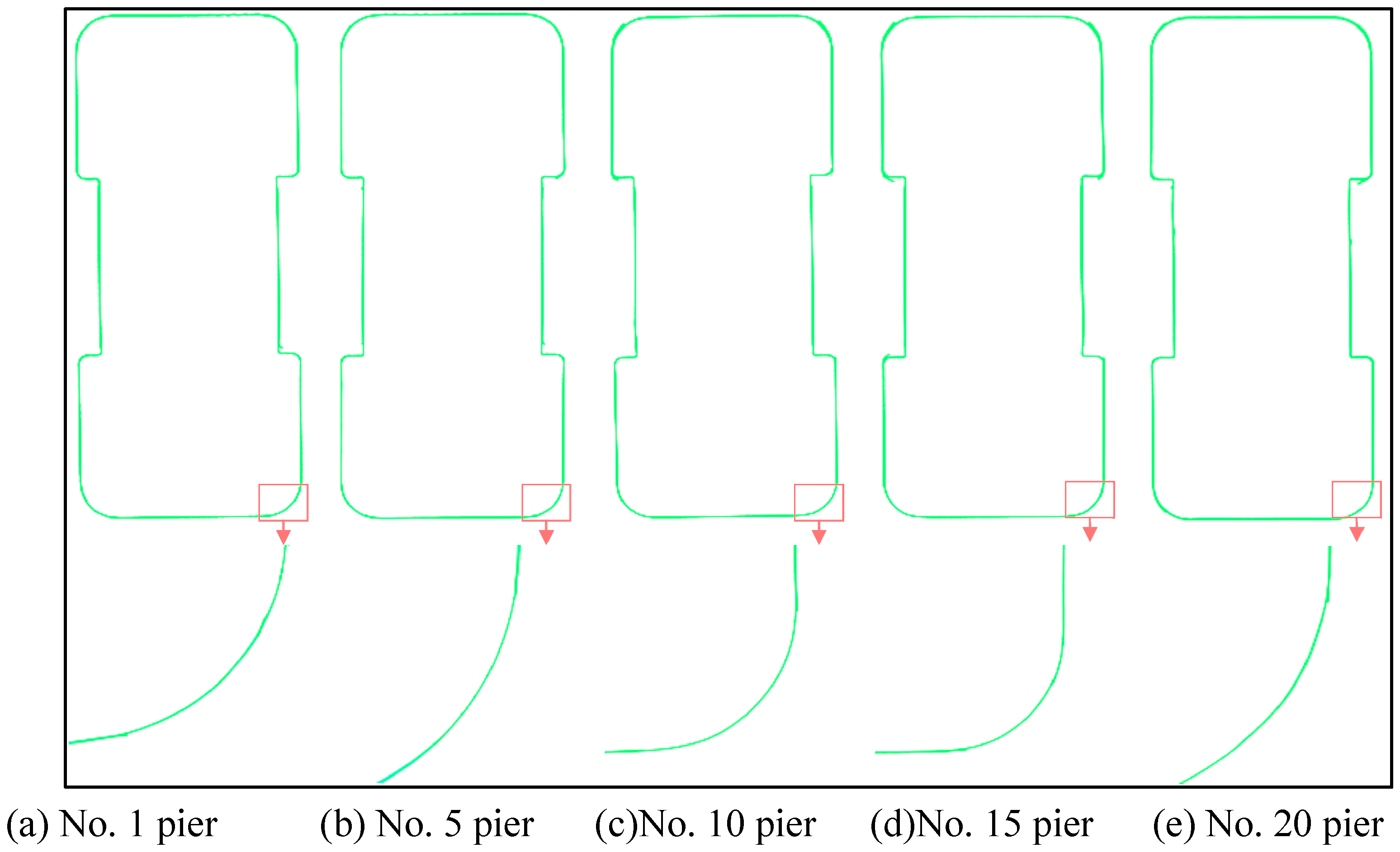
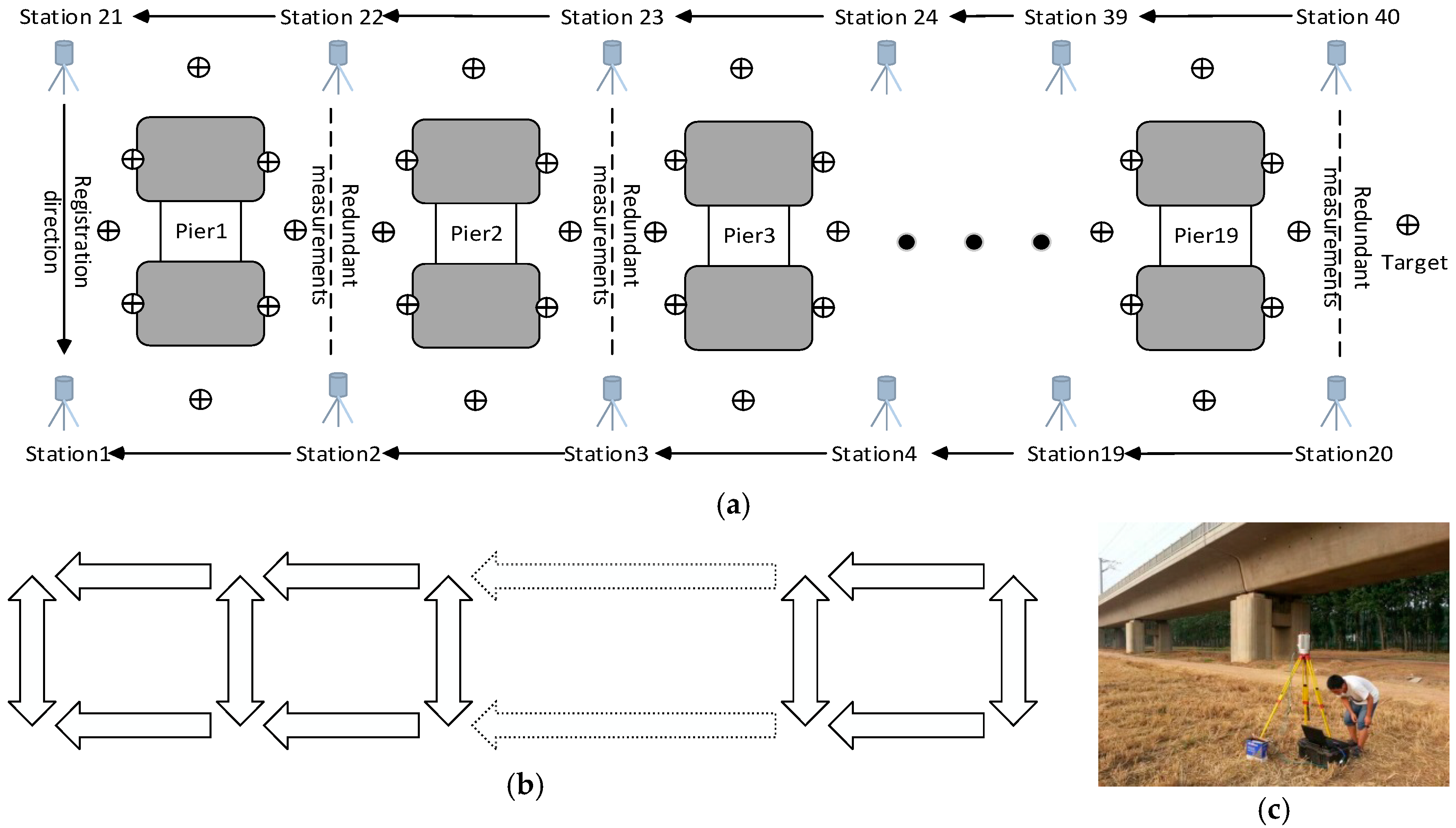
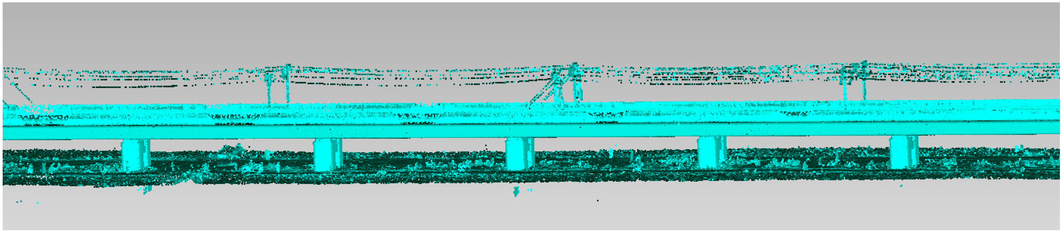
4.1. Experimental Scene and Device Description

The objective is to measure the high-speed rail bridge piers using TLS data. The TLS data facilitate the measurements of railway bridge piers in two aspects. First, multiple scans complete the overall high-speed rail measurements for the long ribbon distributed piers. Second, since the shape of each pier is consistent, analyzing the results of the final registration is useful and extendable. The scanning scene (Figure 2) shows the approximate distribution of scanners and piers. Normally the distance between piers is 30 to 50 m, and the scanner from the nearest pier is 10 to 30 m.
In the experimental scene design, the length of the high-speed rail is 700 m, and two scanning strips (lines of scanning position) are laid in parallel along both sides of the rail. Redundant observations are obtained on both sides of the pier through the piers. The specific conditions for the scanning positions and targets (Figure 2), illustrate the schematic diagram of the scanning positions and the locations of the targets (Figure 2a), the schematic diagram of registration (Figure 2b), and the pier of bridge for HSR (Figure 2c). In Figure 2b, the one-way arrows represents the necessary observations, and the bidirectional arrows represent the redundant observations. All scanning positions are eventually shown as the chain distribution, ensuring the greatest degree of reliability for the scanning position registration. To ensure the stability of the local scanning position registration, at least six target points (radius 5 cm) are laid between the two adjacent scanning positions. The spatial locations of the targets are evenly distributed and considered in the scanner angle of incidence in the layout process for the targets.
A RIEGL VZ-400 V-Line® 3D TLS system is used to scan the pier of HSR viaducts. The key specifications of the RIEGL VZ-400 are based on the product manual [33] as are the accuracy (5 mm) and precision (3 mm). Actual factors that affect the measurement result are the degree resolution of scanning and distance of scan positions. Considering the point density and time cost, the high-speed scan mode (125,000 points/s) was selected for the survey. The density is approximately 1 cm point at the distance of 10 m from scanning position.

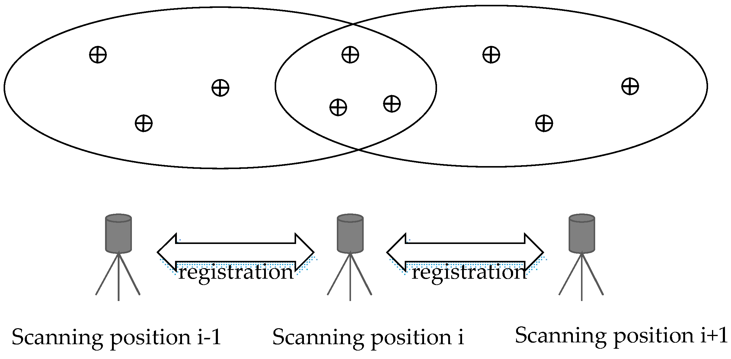
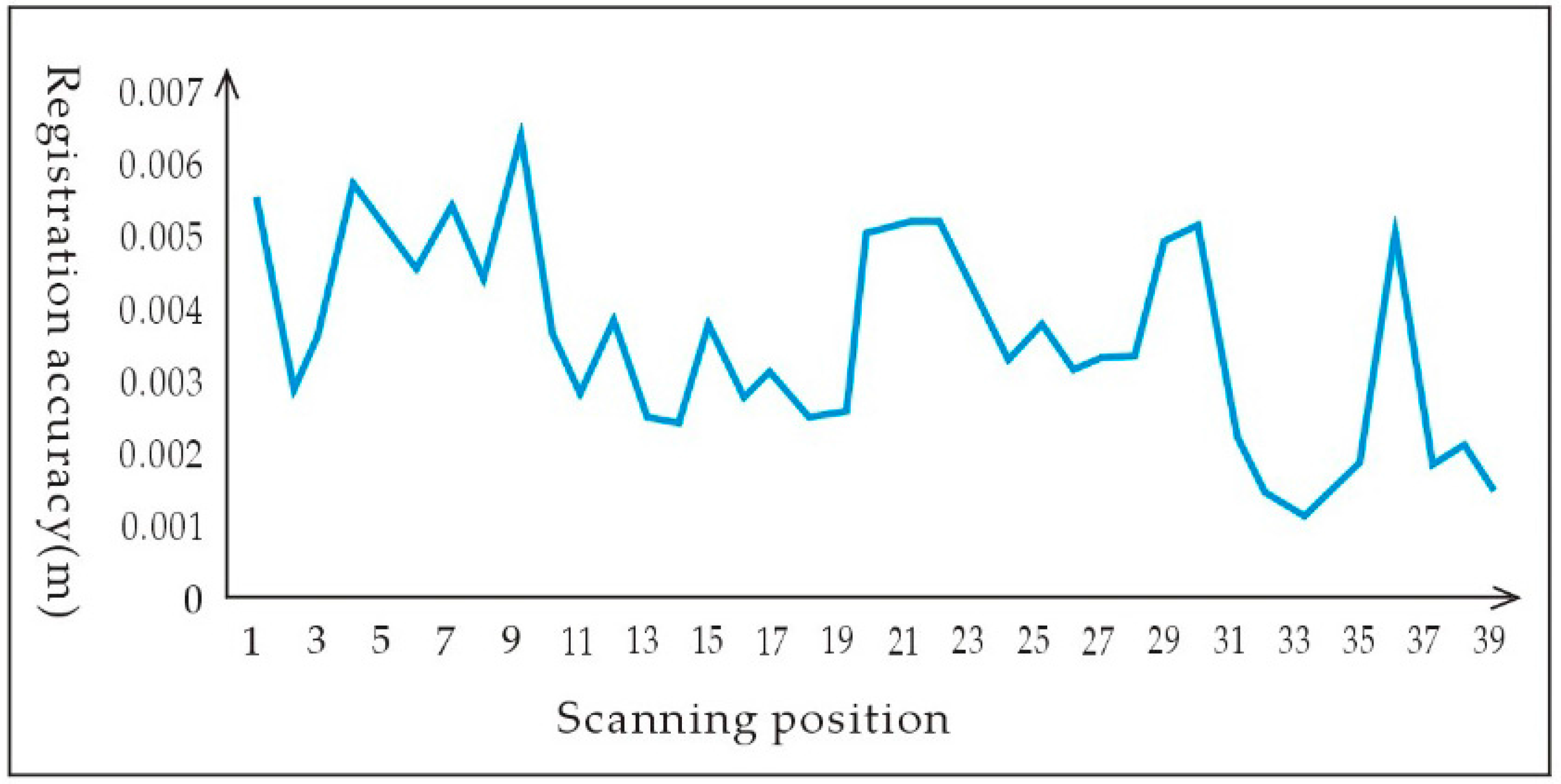
4.2. Registration Test between the Adjacent Scanning Positions

Registration between any two scanning positions (Figure 3) is linked between the scanning positions by the targets. According to the above-described RANSAC algorithm, corresponding points (target inside the ovals of Figure 3) are found between adjacent scanning positions. The adjustment principle solves the rotation and translation matrix to calculate all neighboring scanning positions along the registration line.
The higher precision and greater stable accuracy is achieved for registration of point cloud between the adjacent scanning positions in a small area by using RANSAC algorithm (Figure 4).

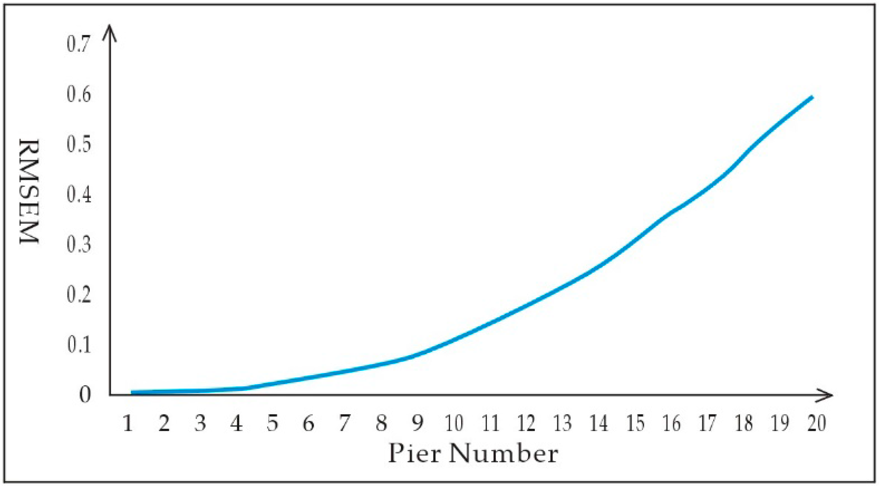
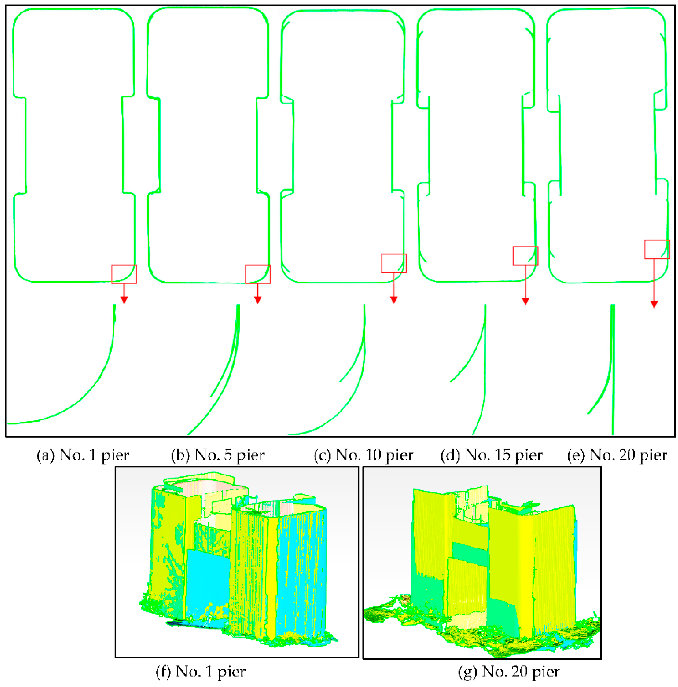
4.3. Registration Experiment for all Scanning Positions

4.3.1. Registration Experiment Using Adjustment Processing

The process of registration for all scanning positions includes three steps as follows: (1) calculating the rotation matrix and translation vector for all scanning positions; (2) incorporating the data of all scanning positions into the scanning coordinate system of the first scanning position by the Equation (7); and (3) calculating the coordinate system for all scanning positions.
In the experimental scene design, a number of targets are selected between each bridge opening (e.g., target of No. 20 scanning position and No. 40 scanning position) (Figure 2a). Since these target coordinates are registered along different routes to the base scanning positions, the coordinate values change after assigning them to the unified coordinate system. The difference of the coordinate value is the misclosure of three-dimensional scanning position, where these are referred to as “check points”. The tested equation for misclosure through these check points is shown in Equation (11):
[ V x V y V z ] = Q 1 Q 2 Q n [ X A Y A Z A ] Q 1 Q 2 Q m [ X B Y B Z B ]
where Q i is the rotation and translation matrix between No. i and No. ( i + 1 ) scanning positions, ( X A , Y A , Z A ) , ( X B , Y B , Z B ) are the coordinates in two scanning coordinate system for the same check point coordinates, and ( V X , V Y , V Z ) is the components of ( X , Y , Z ) for the misclosure of the point. The Root Mean Square Error of the Misclosure (RMSEM) is described in Equation (4).
The coordinates of the same check points put into the unified coordinate system should be the same. An obvious misclosure is formed at the “head-tail” positions due to the spread of registration errors. After calculating the errors for all the targets put into a unified coordinate system on all the bridge opening along the measuring direction, the RMSEM is calculated (Figure 5).
The RMSEM is accumulated rapidly with an increase in the number of scanning positions in the closed loop. The RMSEM growth and its impact on the scan data registration are illustrated in Figure 6a–e, followed by the sectional view of the piers of No. 1, No. 5, No. 10, No. 15, and No. 20. Since the surface of each pier is obtained by registering the scan data from different scanning positions, the best method to evaluate the registration results is to verify whether the pier surface is fusioned well. There are small misclosures on No. 1 and No. 5 piers (Figure 6), indicating that the scanning data are integrated well from different scanning positions. With the accumulation of errors, the scanning data cannot be merged, and the dislocation is increasingly serious. The overall screenshot of the No. 1 piers (Figure 6f), where different colors represent different points from the scanning positions shows that the registration precision is high, and the external surface of the pier is shown well. The overall shot of the No. 20 pier (Figure 6g) is a seriously distorted model.

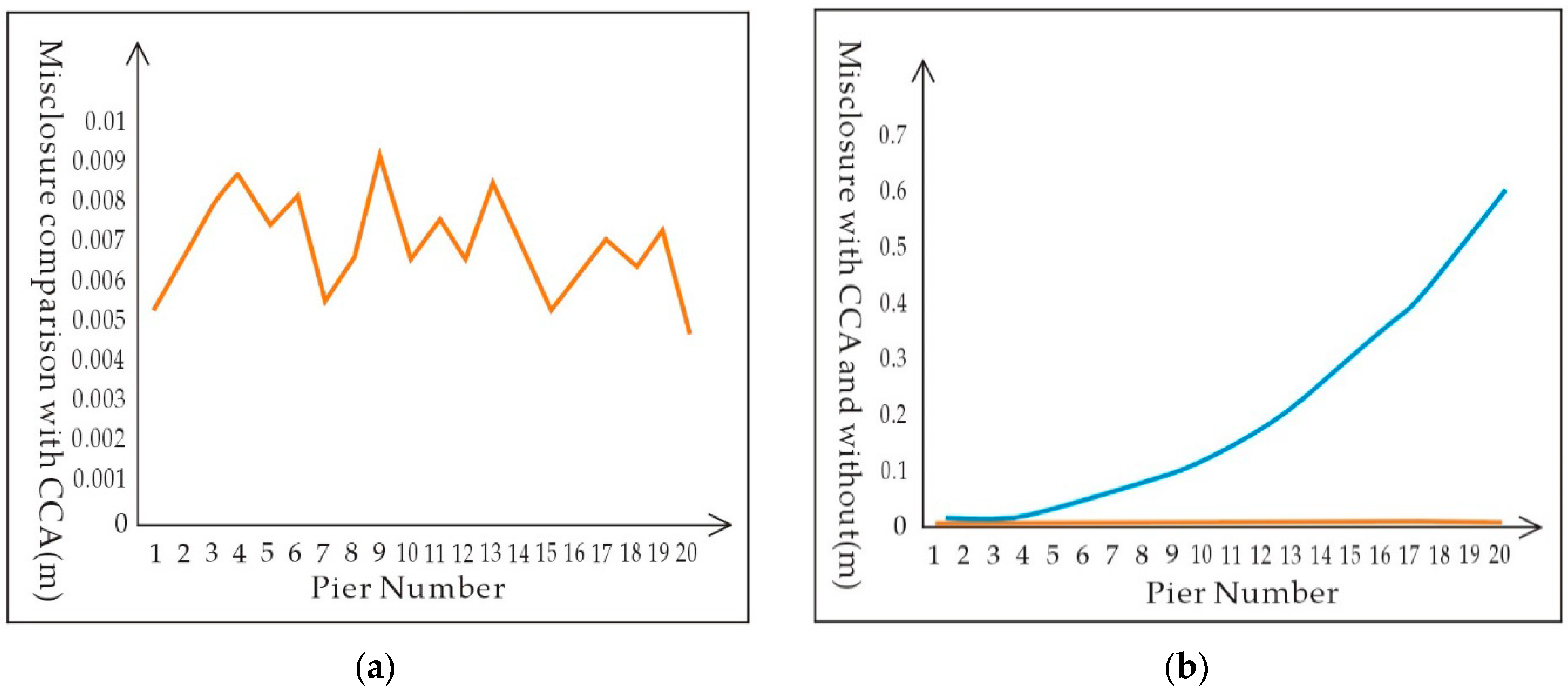
4.3.2. The CCA Experiment

In the above experiment, the ordinary registration method is not suitable for large-scale registration. In the most distant measurements, the pier model has serious deformities, which affect the use of data subsequently. Therefore, the integrity of the measurement object model is not guaranteed. In this experiment, the redundant observation conditions are integrated into the complete adjustment (Section 3.3). The rotation and translation matrix is recalculated for each station and used for registration again. The RMSEM changes, where (a) is the RMSEM value along the measuring direction with CCA and (b) is the comparison chart for the RMSEM between without and with CCA is illustrated (Figure 7). The effectiveness of the adjustment process shows that the RMSEM after adjustment is <0.01 m, far less than 0.59 m before adjustment.
For comparison, the registration results without CCA (Figure 8) is given to the sectional view of the pier of No. 1, No. 5, No. 10, No. 15, and No. 20 by using adjustment for registration. All the piers are well merged without rough surface or obvious dislocation (Figure 8). The result of 3D points cloud of piers of complete registration is illustrated (Figure 9).

5. Concluding Remarks

A RANSAC-based TLS registration algorithm and an indirect adjustment principle were presented to co-register scanned data. In large-scale target scanning position registration, the accumulation of errors has a significant impact on data usage and produces a distorted final registration result. For a pier feature in particular, a layout method for the target points is presented that is suitable for registration of long-strip pier data. The closing condition adjustment significantly reduces the accumulated error and produces useful results. In addition, a closing condition for the complete adjustment methodology was introduced and experiments were conducted to verify the method’s efficiency.
Using RANSAC to register point cloud generally meets the corresponding accuracy requirements. The registration precision for the adjacent scanning positions can achieve 1 mm–6.5 mm. Due to the spread of registration errors, the misclosure is accumulated rapidly up to 0.6 m with the increase of the number of measurement scanning positions in the closed loop, which hampers the merger of the scanning data and leads to dislocation. The pier model has major deformities at the start and end of the measurements, which affects the data’s utility. Here, the RANSAC-based registration, combined with CCA to eliminate the accumulated registration errors, is proposed. The effectiveness of the adjustment process by comparison experiments shows that the RMSEM with CCA is less than 0.01 m, far less than 0.59 m before adjustment. In addition, all cloud point data of the piers are merged without rough surface or obvious dislocation. The experimental registration shows that the method significantly improves the long-strip registration. This methodology is a better solution to eliminate accumulated error within a certain length. When it is longer (more than 30 scanning positions), this constraint is not strong enough and needs to be controlled by the external control points.
Future research issues that emerge from our approach include the fully automated high-precision registration without using artificial targets. Regarding this particular application of real-time online bridge monitoring, it is critical to reduce the time cost of the automatic registration process. Since laser-scanning instruments are often equipped with an additional image sensor, benefiting from this opportunity to improve registration is another emerging research direction.

Acknowledgments

The authors thank the anonymous reviewers and members of the editorial team for the comments and contributions. This work is supported by National High Technology Research and Development Program of China (2013AA063905) and by the National Natural Science Foundation of China (NSFC) under project number 41001309 and by National Science and Technology Support Program under Grant 2012BAJ23B03.

Author Contributions

Li Zheng originated the idea, conducted the experiments, and wrote the manuscript; Manzhu Yu edited and revised the manuscript. Mengxiao Song and Zheng Ji designed and performed the experiments. Anthony Stefanidis and Chaowei Yang co-designed the presentation, commented on content, and revised the manuscript.

Conflicts of Interest

The authors declare no conflict of interest.

References

  1. Krzyzanowski, M.; Apte, J.S.; Bonjour, S.P.; Brauer, M.; Cohen, A.J.; Prüss-Ustun, A.M. Air pollution in the mega-cities. Curr. Environ. Health Rep. 2014, 1, 185–191. [Google Scholar] [CrossRef]
  2. Xu, J.; Zhang, M. Status and development of terrestrial laser scanner. Bull. Surv. Mapp. 2007, 1, 47–50. [Google Scholar]
  3. Gikas, V. 3D Terrestrial laser scanning for geometry documentation and construction management of highway tunnels during excavation. Sensors 2012, 12, 11249–11270. [Google Scholar] [CrossRef] [PubMed]
  4. Liu, C.; Li, N.; Wu, H.; Meng, X. Detection of high-speed railway subsidence and geometry irregularity using terrestrial laser scanning. J. Surv. Eng. 2014, 140, 3. [Google Scholar] [CrossRef]
  5. Vezocnik, R.; Ambrozic, T.; Sterle, O.; Bilban, G.; Pfeifer, N.; Stopar, B. Use of Terrestrial laser scanning technology for long term high precision deformation monitoring. Sensors 2009, 9, 9873–9895. [Google Scholar]
  6. Wang, C.; Stefanidis, A.; Croitoru, A.; Agouris, P. Map registration of image sequences using linear features. Photogramm. Eng. Remot Sens. 2008, 74, 25–38. [Google Scholar] [CrossRef]
  7. Huising, E.J.; Pereira, L.M.G. Errors and accuracy estimates of laser data acquired by various laser scanning systems for topographic applications. ISPRS J. Photogramm. Remote Sens. 1998, 53, 245–261. [Google Scholar] [CrossRef]
  8. Zheng, D.; Shen, Y.; Liu, C. 3D laser scanner and its effect factor analysis of surveying error. Eng. Surv. Mapp. 2005, 14, 32–34. [Google Scholar]
  9. Fisher, M.; Bolles, R. Random sample consensus: A paradigm for model fitting with applications to image analysis and automated cartography. Commun. ACM 1981, 24, 381–395. [Google Scholar]
  10. Besl, P.J.; Makay, N.D. A method for registration of 3-d shapes. IEEE TPAMI 1992, 14, 239–256. [Google Scholar] [CrossRef]
  11. Habib, A.; Ghanma, M.; Morgan, M. Photogrammetric and LiDAR data registration using linear features. Photogramm. Eng. Remote Sens. 2005, 71, 699–707. [Google Scholar]
  12. Al-Durgham, M.; Detcheve, I.; Habib, A. Analysis of two triangle-based multi-surface registration algorithms of irregular point clouds. Int. Arch. Photogramm. Remote Sens. Spat. Inf. Sci. 2011, 38, 61–66. [Google Scholar] [CrossRef]
  13. Sequeira, V.; Ng, K.; Wolfart, E.; Goncalves, J.G.M.; Hogg, D. Automated reconstruction of 3D models from real environments. ISPRS J. Photogramm. Remote Sens. 2012, 54, 1–22. [Google Scholar] [CrossRef]
  14. Bae, K.; Lichti, D.D. A method for automated registration of unorganised point clouds. ISPRS J. Photogramm. Remote Sens. 2008, 63, 36–54. [Google Scholar] [CrossRef]
  15. Chen, Y.; Medioni, G. Object modeling by registration of multiple range images. Image Vis. Comput. 1992, 14, 145–155. [Google Scholar]
  16. Habib, A.F.; Detchev, I.; Bang, K.I. Comparative analysis of two approaches for multiple-surface registration of irregular point clouds. ISPRS Int. Arch. Photogramm. Remote Sens. Spat. Inf. Sci. 2010, 38, 61–66. [Google Scholar]
  17. Zheng, D.; Yue, D. Geometric feature constraint based algorithm for building scanning point cloud registration. J. Surv. Mapp. 2008, 37, 464–468. [Google Scholar]
  18. Ma, H.; Yao, C. Registration of LiDAR point clouds and high resolution images based on linear features. Geomat. Inf. Sci. Wuhan Univ. 2012, 37, 136–139. [Google Scholar]
  19. Rabbani, T.; Dijkman, S.; Heuvel, F.; Vosselman, G. An integrated approach for modelling and global registration of point clouds. ISPRS J. Photogramm. Remote Sens. 2007, 61, 355–370. [Google Scholar] [CrossRef]
  20. Eo, Y.D.; Pyeon, M.W.; Kim, S.W.; Kim, J.R.; Han, D.Y. Coregistration of terrestrial LiDAR points by adaptive scale-invariant feature transformation with constrained geometry. Autom. Constr. 2012, 25, 49–58. [Google Scholar] [CrossRef]
  21. Sibel, C. Planar and Linear Feature-Based Registration of Terrestrial Laser Scans with Minimum Overlap using Photogrammetric Data. Master’s Thesis, Department of Geomatics Engineering, Calgary University, Alberta, China, 2012. [Google Scholar]
  22. Brenner, C.; Dold, C.; Ripperda, N. Coarse orientation of terrestrial laser scans in urban environments. ISPRS J. Photogramm. Remote Sens. 2008, 63, 4–18. [Google Scholar] [CrossRef]
  23. Jaw, J.J.; Chuang, T.Y. Registration of ground‐based LiDAR point clouds by means of 3D line features. J. Chin. Instit. Eng. 2008, 31, 1031–1045. [Google Scholar]
  24. Huang, T.; Zhang, D.; Li, G.; Jiang, M. Registration method for terrestrial LiDAR point clouds using geometric features. Opt. Eng. 2012, 51, 21111–21114. [Google Scholar] [CrossRef]
  25. Cheng, X.; Shi, G. Research on point cloud registration error propagation. J. Tongji Univ. 2009, 37, 1668–1672. [Google Scholar]
  26. Xu, Y.; Gao, J. Research on point cloud registration error of terrestrial laser scanning. J. Geod. Geodyn. 2011, 32, 129–132. [Google Scholar]
  27. Zheng, M.; Zhang, Y.; Zhu, J.; Xiong, X. Self-Calibration adjustment of CBERS-02B long-strip imagery. IEEE Trans. Geosci. Remote Sens. 2015, 53, 3847–3854. [Google Scholar] [CrossRef]
  28. Ji, Z.; Song, M.; Guan, H.; Yu, Y. Accurate and robust registration of high-speed railway viaduct point clouds using closing conditions and external geometric constraints. ISPRS J. Photogramm. Remote Sens. 2015, 106, 55–67. [Google Scholar] [CrossRef]
  29. Anders, H.; Johan, N. Optimal RANSAC—Towards a repeatable algorithm for finding the optimal set. J. Wscg 2013, 21, 21–30. [Google Scholar]
  30. Hough, P.V.C. Method and Means for Recognizing Complex Patterns. U.S. Patent 3,069,654, 18 December 1962. [Google Scholar]
  31. Isack, H.; Boykov, Y. Energy-Based geometric multi-model fitting. Int. J. Comput. Vis. 2012, 97, 123–147. [Google Scholar] [CrossRef]
  32. Tao, B.; Qiu, W.; Yao, Y. The Base of Errors Theory and Surveying Adjustment; Wuhan University Press: Wuhan, China, 2009; pp. 106–111. [Google Scholar]
  33. RIEGL VZ-400 Data Sheet. Available online: http://www.riegl.com/uploads/tx_pxpriegldownloads/10_DataSheet_VZ-400_2014-09-19.pdf (accessed on 19 September 2014).
Figure 1. Registration flowchart based on RANSAC algorithm.
Remotesensing 08 00278 g001
Figure 2. Scanning scene of experimental data; (a) Schematic diagram of the scanning position and the location of the target; (b) Chain scanning position registration schematic; (c) Pier of bridge for HSR.
Remotesensing 08 00278 g002
Figure 3. A schematic diagram of the adjacent scanning position registration.
Remotesensing 08 00278 g003
Figure 4. Registration accuracy map adjacent scanning positions.
Remotesensing 08 00278 g004
Figure 5. The growth for the RMSEM along the measuring direction.
Remotesensing 08 00278 g005
Figure 6. Comparision of the registration results; (a) No.1 pier; (b) No.5 pier; (c) No.10 pier; (d) No.15 pier; (e) No.20 pier; (f) No.1 pier; (g) No.20 pier.
Remotesensing 08 00278 g006
Figure 7. The comparison of RMSEM. (a) RMSEM with CCA (b) The comparison of RMSEM with and without CCA.
Remotesensing 08 00278 g007
Figure 8. The sectional view of the pier registration by using the adjustment results.
Remotesensing 08 00278 g008
Figure 9. The complete registration results.
Remotesensing 08 00278 g009
Table 1. Comparison of these registration methods.
Initial ValueNeed External Control Using Point CloudUsing Target PointPrecision &Stability Depend on
ICPYesNoYesNo Feature
Geometric Primitive YesNoYesNoFeature
RANSAC & CCANoNo NoYesTarget point

