GLASS Daytime All-Wave Net Radiation Product: Algorithm Development and Preliminary Validation

Abstract

Mapping surface all-wave net radiation (R_n) is critically needed for various applications. Several existing R_n products from numerical models and satellite observations have coarse spatial resolutions and their accuracies may not meet the requirements of land applications. In this study, we develop the Global LAnd Surface Satellite (GLASS) daytime R_n product at a 5 km spatial resolution. Its algorithm for converting shortwave radiation to all-wave net radiation using the Multivariate Adaptive Regression Splines (MARS) model is determined after comparison with three other algorithms. The validation of the GLASS R_n product based on high-quality in situ measurements in the United States shows a coefficient of determination value of 0.879, an average root mean square error value of 31.61 Wm⁻², and an average bias of −17.59 Wm⁻². We also compare our product/algorithm with another satellite product (CERES-SYN) and two reanalysis products (MERRA and JRA55), and find that the accuracy of the much higher spatial resolution GLASS R_n product is satisfactory. The GLASS R_n product from 2000 to the present is operational and freely available to the public.

1. Introduction

Surface all-wave net radiation (R_n), characterizing the available radiative energy at the Earth’s surface that is usually called surface radiation budget, is the difference between total upward and total downward radiation. Mathematically, R_n consists of four components:

$$\begin{array}{l}{R}_n=R_{ns}+R_{nl},\\ R_{ns}=R_{si}-R_{so}=(1-\alpha )R_{si}\\ R_{nl}=R_{li}-R_{lo}\end{array}$$

(1)

where R_ns is the net shortwave radiation, R_nl is the net longwave radiation, R_si is the incident shortwave radiation, R_so is the reflected shortwave radiation calculated by R_so = α*R_si where α is shortwave broadband albedo, R_li is the downward longwave radiation, and R_lo is the outgoing longwave radiation.

R_n drives the processes of evapotranspiration and air and soil heat fluxes, as well as other smaller energy-consuming processes such as photosynthesis [1,2]. R_n is a critical parameter to estimate evapotranspiration [3,4,5]. The net surface radiation controls the energy and water exchanges between the biosphere and the atmosphere, and has major influences on the Earth’s weather and climate [6,7]. Thus, reliable spatial and temporal R_n information is required for many applications. However, in spite of its importance, directly measured R_n is available only from a very small number of standard radiometric observatories because of the expensive instrumentation and constant maintenance needed to guarantee that reliable measurements can be provided [8]; these in situ measurements are thus unable to characterize the spatial variation.

Alternative methods for obtaining R_n are meteorological reanalysis and satellite remote sensing [9].

Table 1. Characteristics of the commonly used R_n datasets.

Product	Spatial Resolution	Temporal Resolution	Period	Reference
Reanalysis products
NCEP/CFSR	T382 (38 km)	6 hourly	1979–2010	[10,12]
NASA/MERRA	$0.5°\times \frac{2}{3}°$	hourly	1979–present	[13]
ERA40	T159 (125 km)	6 hourly	1957–2002	[14]
ERA-Interim	T255 (80 km)	3 hourly	1980–present	[15]
JRA55	T319 (~55 km)	3 hourly	1958–present	[16]
NCEP/NCAR RII	T62 (200 km)	6 hourly	1979–present	[17]
remotely sensed products
CERES-SYN	1°	3 hourly	2000–present	[18]
GEWEX-SRB	1°	3 hourly	1983–2007	[19,20]
ISCCP-FD	280 km	3 hourly	1983–2011	[21]

gives detailed information about the commonly used R_n products. Reanalysis products are usually derived by merging available observations with an atmospheric model to obtain the best estimate of the states of the atmosphere and land surface [10], while existing remote sensing products are generated mostly based on a radiative transfer model with inputted atmospheric and surface parameters. From Table 1, we can see that the spatial resolutions of these products are too coarse for many land applications although they are temporally continuous and globally complete. Another issue is that the accuracies of these products vary considerably and may not meet the application requirements, such as the global change research [9,10,11]. Therefore, a new long-time high-resolution global R_n product with both high accuracy and fine temporal-spatial resolutions is urgently needed.

Many geostationary and polar-orbiting satellite data are at the kilometer spatial resolution and can be potentially used for estimating the individual components of Equation (1), such as incident shortwave radiation [22] and albedo [23,24]. If all components in Equation (1) are known, the calculation of R_n is straightforward [25]. The difficulty in generating the global R_n product using Equation (1) is the estimation of the thermal components under the cloudy conditions. This is the reason why many studies focus primarily only on shortwave [26,27,28] or clear-sky conditions [29]. If we know the exact atmospheric and surface properties, radiative transfer models enable us to calculate surface net radiation. However, it is extremely difficult to generate a complete set of atmosphere and surface products for model calculation at a high resolution. The most practical solution is to estimate incident shortwave radiation directly from satellite observations and then convert it into all-wave net radiation using either linear [30,31,32,33,34] or nonlinear [35,36] models. Jiang et al. [37] recently developed two artificial neuron networks models using comprehensive global in situ observations and found that the nonlinear models can produce better accuracy than the linear models.

The primary objective of this study is to generate the accurate long-term high-resolution Global LAnd Surface Satellite (GLASS) R_n product. The GLASS product suite is for the long-term environmental change studies [38,39] and continuously expanding. For generating such a global product, algorithm development is the key and we must therefore balance the accuracy and computational efficiency of the algorithm. To achieve this objective, we explore two new nonlinear models: Multivariate Adaptive Regression Splines (MARS) and Support Vector Regression (SVR). After comparing them with two models developed earlier [17,20], we select the MARS model to produce the GLASS R_n product at a 5 km spatial resolution. The resulting high-resolution GLASS R_n product is further validated, compared with one satellite product and two reanalysis products. The details are presented in the following sections.

2. Data and Models

2.1. Data

The data used in this study are comprised of in situ radiation measurements, remote sensing products, and meteorological reanalysis data. The remote sensing products and reanalysis data were used to map R_n on a global scale. Based on the characteristics of these data, multiple trial experiments and pre-processing with strict quality control were conducted, and data were aggregated to a daytime or diurnal scale. The variables considered in this study are shown in

Table 2. Variables explanation and source.

	Abbr.	Name	Unit	Source
Response variable	Rn	Daytime surface net radiation	Wm−2	In situ
Independent variables	Rsi	Daily surface incoming solar radiation	Wm−2	In situ
	Rsi*	Daily surface incoming solar radiation	Wm−2	Remotely Sensed data (GLASS products)
	ABD	Daily surface albedo
	NDVI	Daily Normalized Difference Vegetation Index
	Ta	Daytime air mean temperature	°C	Reanalysis product (MERRA)
	Tmin	Daytime air minimum temperature	°C
	Tmax	Daytime air maximum temperature	°C
	PS	Daytime surface air pressure	Pa
	W	Daytime wind speed	ms−1
	RH	Daytime mean relative humidity	%	Calculated
	ea	Daytime water vapor pressure	KPa
	dr	Inverse relative Earth−Sun distance
	CI	Clearness Index
	BI	Brightness Index

R_si* stands for the GLASS R_si product and was used for global GLASS daytime R_n production in this study.

. The readers are referred to Jiang et al. [37] for more information about these data.

As described above, more than 8000 validation samples were selected from the observations made in 2008, and most of them were from 25 sites.

Table 3. Information about the 25 validation sites.

Site	Lat, Lon	Land Cover	Height (m)	Project
Larned, Kansas: E01	$38.20°N,99.32°W$	Cropland	632	ARM
LeRoy, Kansas: E03	$38.20°N,95.60°W$	Cropland	338	ARM
Plevna, Kansas: E04	$37.95°N,98.33°W$	Rangeland	513	ARM
Halstead, Kansas: E05	$38.11°N,97.51°W$	Wheat	440	ARM
Towanda, Kansas: E06	$37.84°N,97.02°W$	Alfalfa	409	ARM
Elk Falls, Kansas: E07	$37.38°N,96.18°W$	Pasture	283	ARM
Coldwater, Kansas: E08	$37.33°N,99.31°W$	Rangeland	664	ARM
Tyro, Kansas: E10	$37.07°N,95.79°W$	Alfalfa	248	ARM
Byron, Oklahoma: E11	$36.88°N,98.29°W$	Alfalfa	360	ARM
Pawhuska, Oklahoma: E12	$36.84°N,96.43°W$	Prairie	331	ARM
Lamont, Oklahoma: E13	$36.61°N,97.49°W$	Pasture	318	ARM
Ringwood, Oklahoma: E15	$36.43°N,98.28°W$	Pasture	418	ARM
El Reno, Oklahoma: E19	$35.56°N,98.02°W$	Pasture	421	ARM
Meeker, Oklahoma: E20	$35.56°N,96.99°W$	Pasture	309	ARM
Okmulgee, Oklahoma: E21	$35.62°N,96.07°W$	Forest	240	ARM
Cordell, Oklahoma: E22	$35.35°N,98.98°W$	Rangeland	465	ARM
Cyril, Oklahoma: E24	$34.88°N,98.21°W$	Wheat	409	ARM
Earlsboro, Oklahoma: E27	$35.27°N,96.74°W$	Pasture	300	ARM
Bondville: SF_BND	$40.05°N,88.37°W$	Cropland	230	SURFRAD
Boulder: SF_TBL	$40.13°N,105.24°W$	Grassland	1689	SURFRAD
Desert Rock: SF_DRA	$36.63°N,116.02°W$	Desert	1007	SURFRAD
Fort Peck: SF_FPK	$48.31°N,105.10°W$	Grassland	634	SURFRAD
Goodwin Creek: SF_GCM	$34.25°N,89.87°W$	Grassland	98	SURFRAD
Penn. State: SF_PSU	$40.72°N,77.93°W$	Cropland	376	SURFRAD
Sioux Falls: SF_SXF	$43.73°N,96.62°W$	Shrubland	473	SURFRAD

gives detailed information about these sites, which were mainly from the ARM (http://www.arm.gov/) and SURFRAD (http://www.srrb.noaa.gov; [40]) observation networks. This ensures that the data are of the best quality currently available. The distribution of the 25 sites is shown in Figure 1. All ARM and SURFRAD data are carefully checked, and quality-control information is supplied with the data (ftp://aftp.cmdl.noaa.gov/data/radiation/surfrad/) and http://www.archive.arm.gov/; [41]).

2.2. Methods

The overall flowchart of this study is shown in Figure 2. First, the GLASS R_n algorithm was determined by comparing four R_n estimation models (Section 3), including the multivariate adaptive regression splines (MARS), the support vector regression (SVR) model, a linear regression model (LM) [21], and a general regression neural network (GRNN) model [20]. To the best of our knowledge, the first two models are the first to be applied for estimating surface net radiation. The details of the MARS model are introduced in this section, while the other three models are outlined in the Appendix. After validation and inter-comparison, the MARS model was determined to generate the GLASS daytime R_n product. Second, the MARS model was applied to the all-wave daytime R_n product by converting the GLASS R_si product using other satellite products (e.g., NDVI and albedo) and meteorological information from MERRA (Section 4.1). Finally, the accuracy of the new GLASS R_n product was evaluated by validating it against the site observations and comparing it with other R_n products: one remotely sensed product (CERES-SYN), and two reanalysis products (MERRA and JRA55) (Section 4.2).

MARS is a nonlinear and nonparametric regression model proposed by Friedman [42]. MARS is a generalization of the stepwise linear regression procedure for fitting an adaptive nonlinear regression to data. It is more flexible in modeling relationships that are nearly additive or involve interactions with variables. MARS uses expansions in piecewise linear basis functions of the form:

$$\begin{array}{l}{(x-t)}_{+}=\{\begin{array}{cc}x-t& x>t\\ 0& x\le t\end{array}\\ and\\ {(x-t)}_{-}=\{\begin{array}{cc}t-x& x<t\\ 0& x\ge t\end{array}\end{array}$$

(2)

with x = t being a knot (linear splines). The smoothing function f is a linear expansion of the basic functions,

$$f(x)={\displaystyle \sum _{j=1}{\theta }_j{h}_j(x_j)}$$

(3)

where $h_j(x_j)$ are the piecewise linear basis functions and ${\theta }_j$ are the coefficients that are estimated by minimizing the residual sum-of-squares using standard linear regression.

In this study, MARS was first applied for daytime R_n estimation. It was implemented on the R platform with the package “mda,” in which the input variables can be selected automatically. After extensive experiments, the maximum interaction degree between variables in MARS was set to 2, and the backward stepwise process was carried out to train the MARS model.

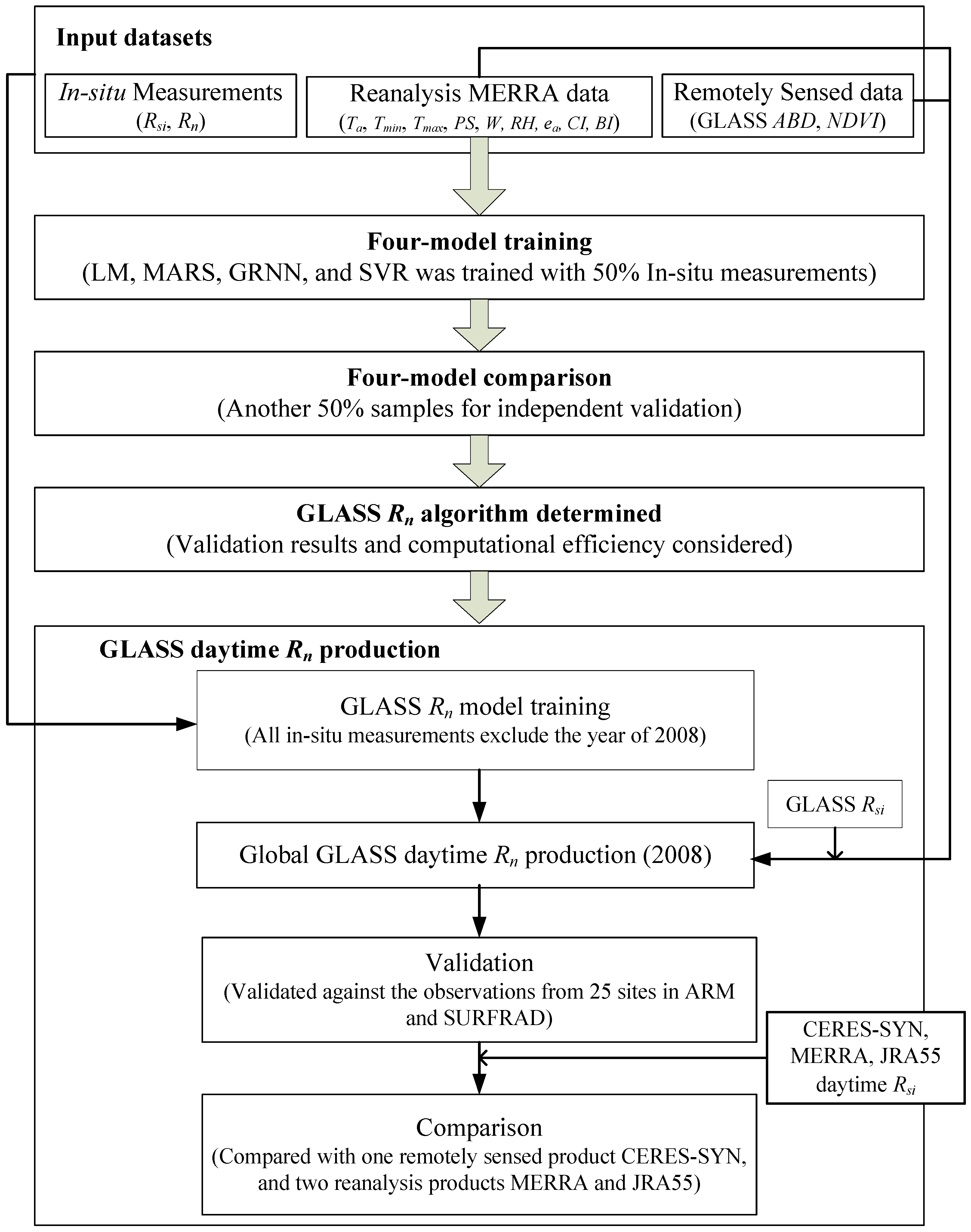
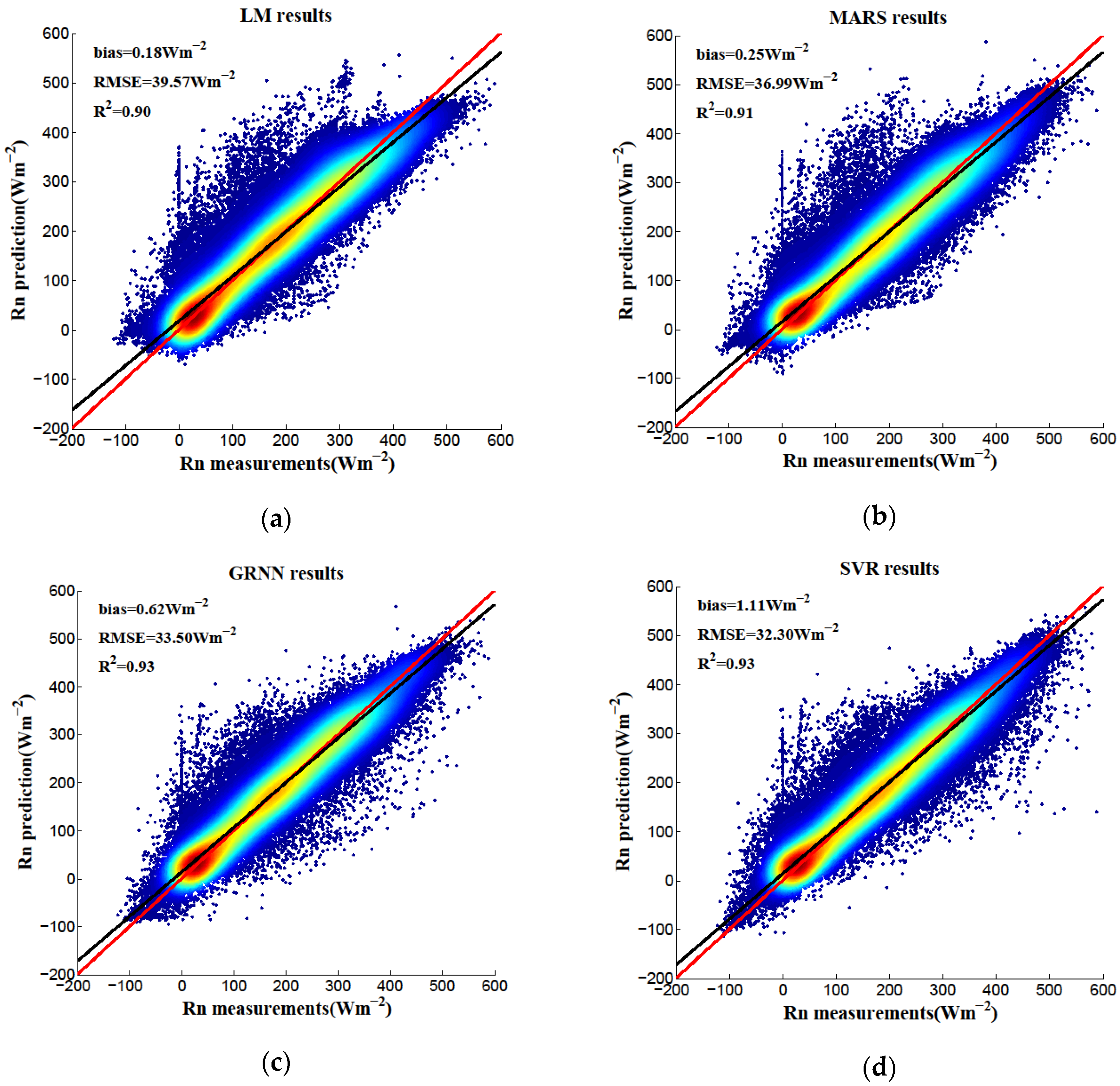
3. GLASS Daytime R_n Algorithm

The four models (LM, MARS, GRNN, and SVR) were trained one by one with half of the total number of in situ measurements and their corresponding reanalysis and satellite datasets (Figure 2). Four predictions were then produced by the other part of the independent validation dataset and compared. The results are shown in Figure 3 and summarized in

Table 4. The statistic results of the four models.

	R2	RMSE (Wm−2)	Bias (Wm−2)	Training Time	Fitting Time
LM	0.90	39.57	−0.18	<60 s	<60 s
MARS	0.91	36.98	−0.26	<60 s	<60 s
GRNN	0.93	33.49	−0.62	>72 h	>72 h
SVR	0.94	32.28	−1.11	>72 h	>48 h

. Three measurements of the fitting statistics were compared: R-square (R²), root mean square error (RMSE), and bias. The computational times are also given in Table 4 for better comparison. In the present study, all the models were implemented under the Microsoft Windows 7 system on a Intel Core 3.20 GHz PC with 8 GB memory.

Based on these comparison results (mainly R² and RMSE values since the bias values are relatively small), it is clear that the predictive abilities of the GRNN and SVR models were similar and also better than those of the other two models. The LM model performed the worst and the MARS model’s performance was intermediate. However, the computational times for model training and fitting differed considerably between the four models (see Table 4). In short, the computational efficiencies of the GRNN and SVR models were very low when large datasets were applied, and these two models are unsuitable for generating the long-term GLASS daytime R_n product. Extensive experiments were then performed to determine if the sample sizes could be reduced without decreasing the data fitting accuracy using these two machine learning models. Taking the SVR model as an example, it was found that the fitting accuracy linearly decreased when the training samples were reduced in size (

Table 5. Fitting accuracy in SVR with different sample sizes.

Sample Size	R2	RMSE (Wm−2)	Bias (Wm−2)
218,516	0.94	32.28	−1.11
22,298	0.93	34.22	−2.23
11,395	0.92	35.62	−2.73
7755	0.92	36.01	−2.06

), resulting in a data fitting accuracy very close to the result of the MARS model (Table 4) when the time for training and fitting was acceptable. The situation for the GRNN model was similar. Given the trade-off between computational time and prediction accuracy, the MARS model was accepted as the first option for GLASS daytime R_n production.

To achieve a better understanding of the applicability of the MARS model, all samples were grouped into four categories in accordance with Jiang et al. [43], and the prediction accuracy of the MARS model for these four categories was compared. Jiang et al. [43] found that NDVI = 0.2 can be used as the threshold to identify vegetated surfaces, and three more classes can be roughly divided based on albedo according to the different relations between R_si and R_n when NDVI < 0.2 (see

Table 6. Four classifications based on combinations of Normalized Difference Vegetation Index (NDVI) and albedo (see Table 2, with their corresponding numbers of samples.

Class	Classification Criteria	No. of Samples
S1	NDVI < 0.2 and albedo ≤ 0.25	8967
S2	NDVI < 0.2 and 0.25 < albedo < 0.7	8317
S3	NDVI < 0.2 and albedo ≥ 0.7	10,064
S4	NDVI ≥ 0.2	167,739

). The comparison fitting results are shown in

Table 7. Validation statistics for the MARS model for these four categories.

	S1	S2	S3	S4
R2	0.87	0.54	0.13	0.91
RMSE (Wm−2)	42.89	47.46	18.21	36.81
bias (Wm−2)	−0.13	0.51	−0.53	−0.28

. In general, the four categories correspond to the major land cover types found on Earth: S1–wetland; S2–desert or barren land with sparse vegetation; S3–snow/ice; and S4–the remaining vegetated surfaces. Furthermore, the seasonal information can also be represented by these categories. The results shown here were similar to our previous study [43] whereby the simulation accuracies are much better for S1 and S4, because the R_si is the dominant factor for R_n for these two categories. Keep in mind that the statistical values are considerably different for snow/ice surfaces (S3) due to the high albedo and clustering of all points. The results proved the robustness of the MARS model in R_n estimation.

4. GLASS R_n Daytime Product Generation

4.1. GLASS Daytime R_n Product

After the MARS model was chosen as the GLASS daytime R_n algorithm, the global GLASS daytime R_n product was generated and evaluated. For the global data production, the GLASS R_si product was applied as the input instead of the in situ R_si measurements. The GLASS R_si product was generated from multiple polar-orbiting and geostationary satellite datasets with a look-up table algorithm. The validation results demonstrated that this product was superior to other products [44]. The instantaneous 3-hourly GLASS R_si was first aggregated into a daytime temporal scale, then the climatic factors from the MERRA reanalysis product were resampled into 5 km spatial resolution to match the GLASS R_si. The GLASS NDVI and GLASS ABD products were also used as inputs. Their spatial resolution is 5 km but temporal resolution is eight-day; therefore, each day during the eight-day period was set to be the same, assuming little variation at the surface over the period.

More than 8000 samples from 25 sites in 2008 were extracted for independent validation of the GLASS daytime R_n product. All other samples from 251 sites were used for the MARS model training. The MARS model was then used to produce the GLASS daytime R_n product. Finally, the GLASS daytime R_n product from 2000 to the present with spatial resolution 0.05 deg (~5 km) in global coverage was generated in this study.

Figure 4b shows the GLASS daytime R_n in day 274 of 2008 (30 September 2008), a randomly selected date. The MERRA daytime R_n for the same day is also shown in Figure 4a for comparison. From the two plots, we concluded that the spatial distribution of R_n is visually similar between the two products, but large discrepancies occur over many regions, such as the northern part of South America and over the Chinese mainland. In addition, the GLASS daytime R_n product gives more details compared with the MERRA dataset because of its higher spatial resolution. To identify which product is more accurate, more validation results of the two products compared with the site observations will be provided in Section 4.2. Note the missing values over part of the Arctic region and the entire Antarctic region due to the missing inputs of the GLASS R_si product.

4.2. Validation and Comparison

For further evaluation, one remotely sensed product (CERES-SYN) and two model reanalysis products (MERRA and JRA55) were used for inter-comparison with the GLASS R_n product; spatio-temporal information about the datasets is given in Table 1. The CERES-SYN product is obtained by merging CERES observations aboard the NASA Terra and Aqua satellites with radiances observed from five geostationary satellites [18,45]. The MERRA product is provided by NASA’s Global Modeling and Assimilation Office (GAMO); it is designed to integrate with NASA’s Earth Observing System (EOS) satellite data for use in climate analysis [46]. JRA55 is offered by the Japan Meteorological Agency (JMA) by using the TL319 version of JMA’s operational data assimilation system in which several newly available and improved past observations were used. JRA55 is recognized as an upgrade to JRA 25 and is considerably better than JRA25 [16,47]. After transferring to the local time of each pixel, the three products were integrated into a daytime temporal scale according to the sunrise and sunset time, and then, along with the GLASS daytime R_n product, they were validated against the respective in situ measurements; the results are shown in Figure 5.

Based on the results, the GLASS and CERES-SYN daytime R_n products were superior to the other two reanalysis products, MERRA and JRA55. By comparing the average RMSE and bias values, it becomes clear that the GLASS daytime R_n product is better than the CERES-SYN product. The average RMSE of GLASS daytime R_n was 31.61 Wm⁻² and the average bias was −17.59 Wm⁻², compared to 35.58 Wm⁻² and −31.00 Wm⁻² for CERES-SYN’s average RMSE and average bias. Comparison also showed that the GLASS product had increased low values and decreased high values (Figure 5a), whereas the CERES-SYN product was larger overall than the measurements (Figure 5b). In addition, the validation accuracy of each site between GLASS and the measurements are shown in

Table 8. Validation results between GLASS daytime R_n and the observations of 25 validation sites.

Site	R2	RMSE (Wm−2)	Bias (Wm−2)	Site	R2	RMSE (Wm−2)	Bias (Wm−2)
E01	0.92	30.00	10.91	E21	0.88	36.24	6.11
E03	0.89	34.20	18.57	E22	0.89	28.62	16.01
E04	0.87	34.54	12.53	E24	0.91	28.52	6.41
E05	0.90	32.78	16.90	E27	0.90	30.51	21.88
E06	0.89	32.19	21.70	SF_BND	0.86	38.26	22.42
E07	0.91	32.16	28.34	SF_DRA	0.67	37.81	10.18
E11	0.92	29.10	17.12	SF_FPK	0.83	37.13	27.34
E12	0.89	32.39	2.74	SF_GCM	0.86	38.12	15.71
E13	0.92	27.42	15.61	SF_PSU	0.88	35.03	34.29
E15	0.92	28.07	18.15	SF_SXF	0.88	37.85	18.18
E19	0.91	27.36	16.48	SF_TBL	0.75	42.35	20.89
E20	0.91	28.65	22.32

. The R² values of most sites were larger than 0.85, the RMSE values were mostly around 30 Wm⁻², and the bias values were chiefly smaller than 25 Wm⁻², thereby demonstrating that the accuracy of the GLASS daytime R_n product is satisfactory with most applications.

Two site examples are also given in Figure 6. Here, the CERES-SYN product was selected because of its best performance among the three products. The two plots show that the GLASS daytime R_n matched the site observations very well and that the CERES-SYN product was larger than the measurements and the GLASS product although the variations were reasonable. Overall, the GLASS daytime R_n product has the potential to be one of the best R_n products available for future applications.

5. Summary

A new R_n product that offers high spatiotemporal resolution, high accuracy, and global coverage over long time periods is urgently needed for a variety of applications. To achieve this goal, we developed the GLASS daytime R_n product. To determine the GLASS daytime R_n production algorithm, four models (LM, MARS, GRNN, and SVR) that convert incident shortwave radiation to all-wave net radiation were trained for R_n estimation and validated with high-quality measurements made in the United States. The validation results indicate that the GRNN and SVR models had the best prediction accuracy over the other two empirical models, although it was unacceptably time consuming, and that the performance of the MARS model is promising. A further experiment also demonstrated that the MARS model is robust under various conditions. Therefore, as a result of the trade-off between the practical requirements of applications and data fitting accuracy requirements, the MARS model was selected as the final GLASS daytime R_n product algorithm. Finally, a global coverage GLASS daytime R_n product with a 5 km spatial resolution and daytime temporal resolution in 2008 was generated using the MARS model.

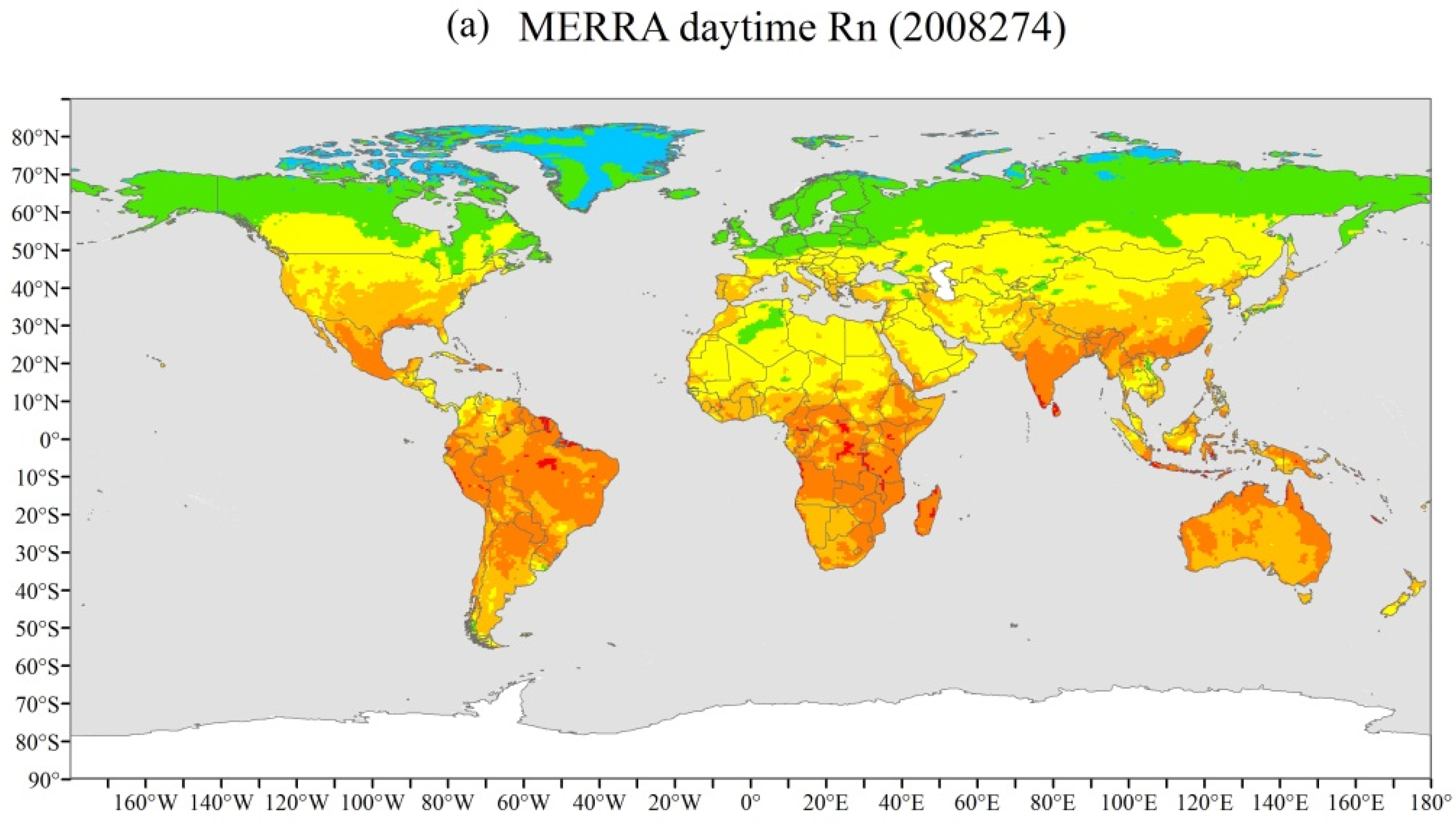
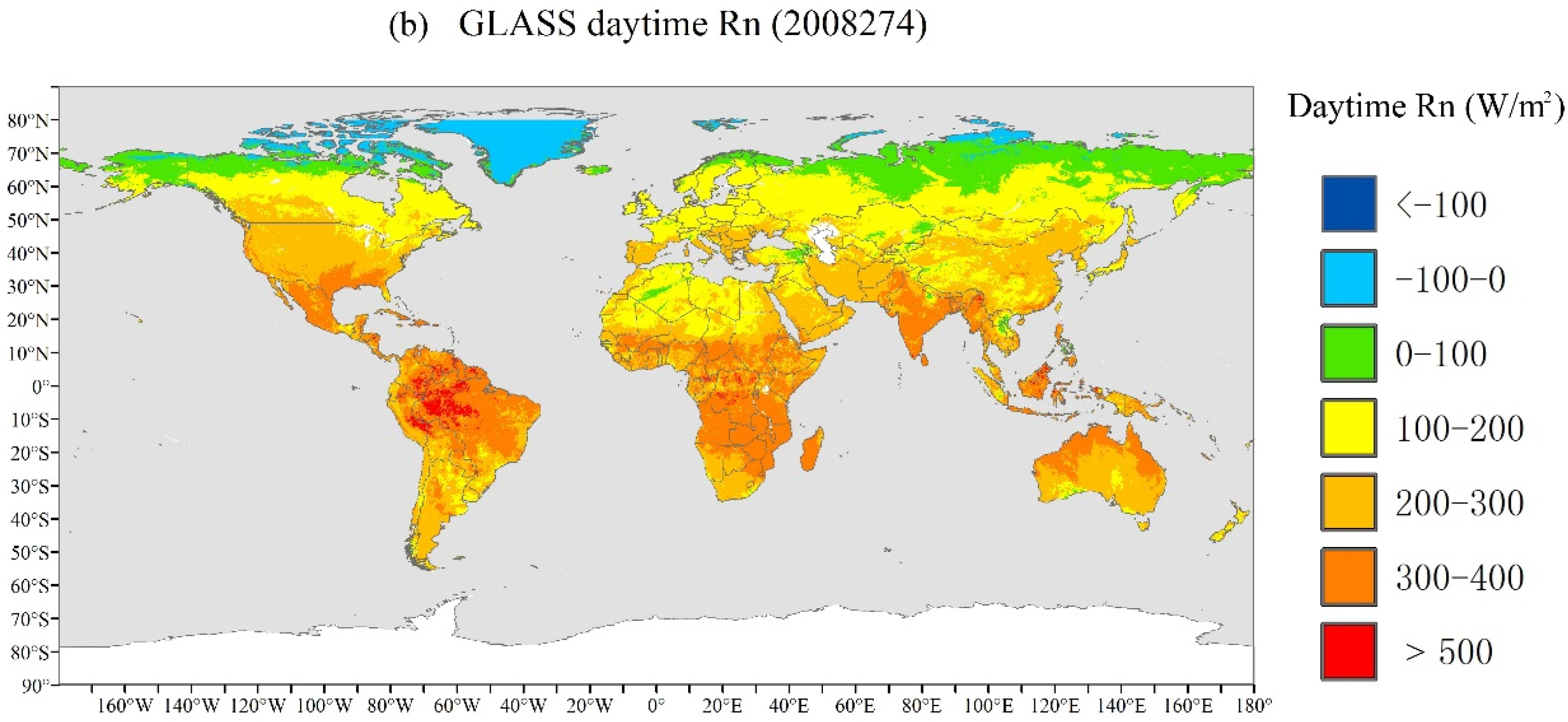
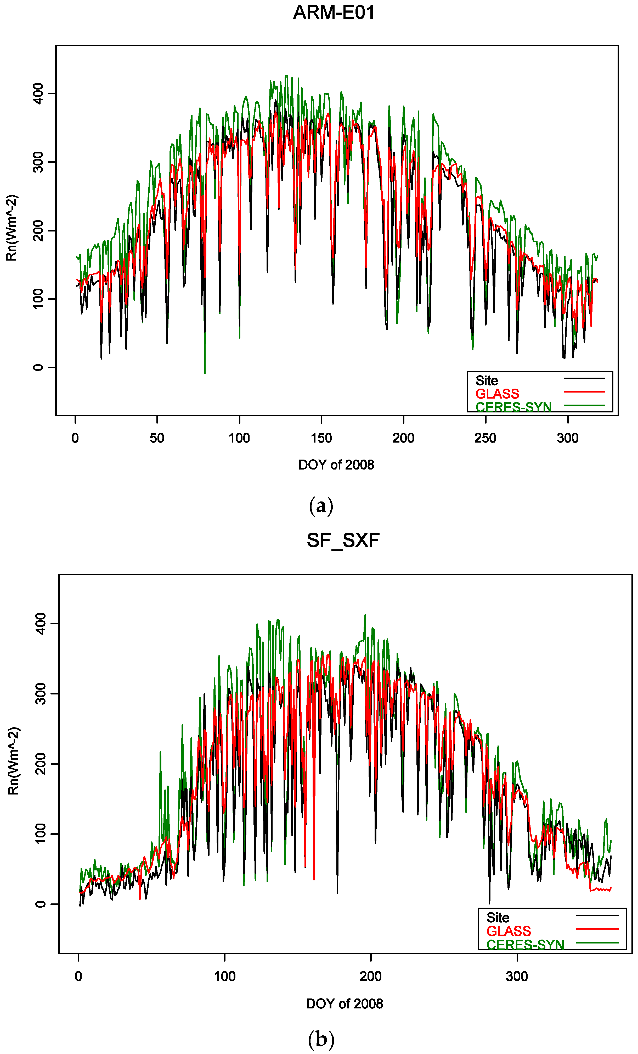
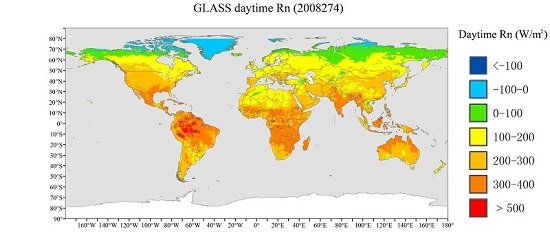
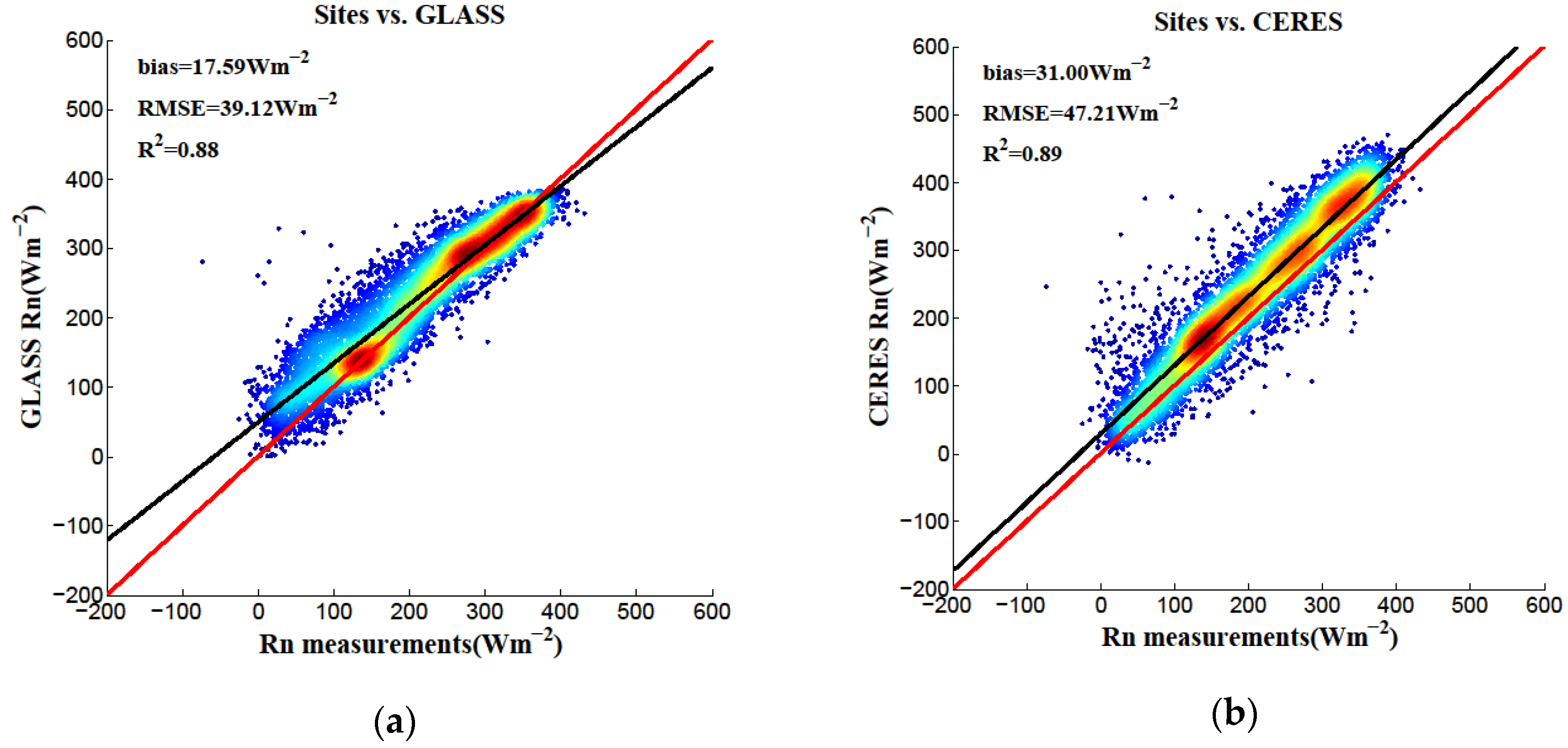
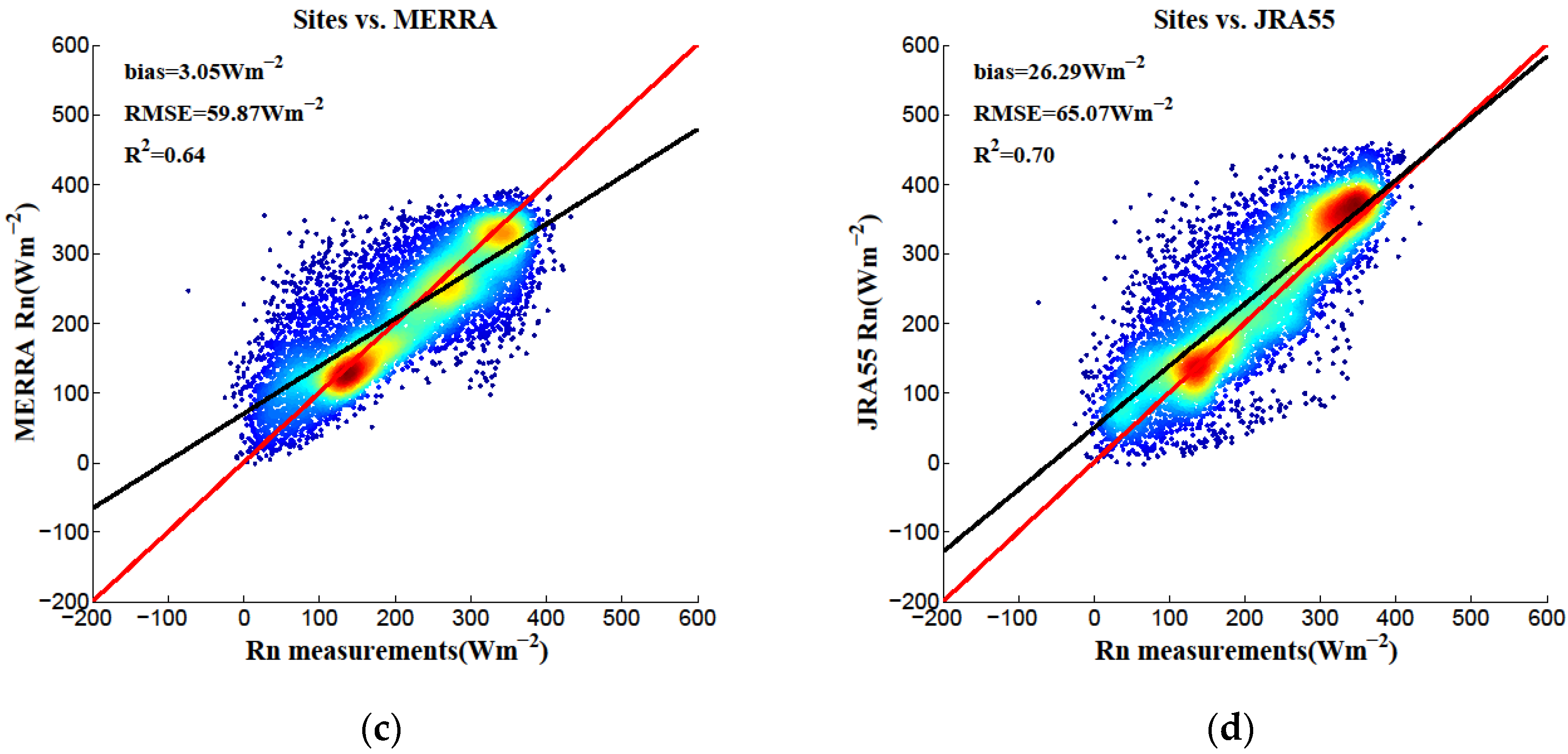
The new daytime R_n product was validated against measurements from 25 independent sites, and was also compared with one remotely sensed R_n product, CERES-SYN, and two reanalysis R_n products, MERRA and JRA55. The validation results illustrate that the new GLASS daytime R_n product delivers more detail at the global scale due to its relatively high spatial resolution and does so without spatial gaps, except for the Arctic and Antarctic regions, and that it has a continuous time series because the all-sky conditions were considered in the MARS algorithm and the GLASS incident shortwave radiation product. The validation results of the GLASS daytime R_n product at the 25 sites were very satisfactory with most applications, with an overall coefficient of determination of 0.88, an average RMSE of 31.61 Wm⁻², and an average bias of 17.59 Wm⁻². The results of comparing the GLASS with three other products also proved that this new daytime R_n product performed much better than the two reanalysis products and similar to CERES-SYN but with a much higher spatial resolution. Overall, the results in the present study show that the GLASS daytime R_n product generated by the MARS model is superior to other presently available products.

Although it is common practice in the literature, validating satellite products and reanalysis datasets at a spatial resolution scale from a few to hundreds of kilometers using “point” ground measurements directly provides questionable results. It is valid only if the atmospheric and surface conditions are homogeneous. An upscaling process using intermediate-resolution products is necessary for many heterogeneous landscapes and atmospheric conditions [48]. A further project conducted by us for addressing the scaling issue is underway, and the results will be presented in the near future.

References

1. Hurtado, E.; Sobrino, J.A. Daily net radiation estimated from air temperature and noaa-avhrr data: A case study for the iberian peninsula. Int. J. Remote Sens. 2001, 22, 1521–1533. [Google Scholar] [CrossRef]
2. Rosenberg, N.J.; Blad, B.L.; Verma, S.B. Microclimate—The Biological Environment; Wiley: New Yorker, NY, USA, 1983; pp. 44–45. [Google Scholar]
3. Allen, R.; Tasumi, M.; Trezza, R. Satellite-based energy balance for mapping evapotranspiration with internalized calibration (metric)—model. J. Irrig. Drain. Eng. 2007, 133, 380–394. [Google Scholar] [CrossRef]
4. Wang, K.C.; Dickinson, R.E.; Wild, M.; Liang, S.L. Evidence for decadal variation in global terrestrial evapotranspiration between 1982 and 2002: 1. Model development. J. Geophys. Res. Atmos. 2010, 115. [Google Scholar] [CrossRef]
5. Yao, Y.; Liang, S.; Li, X.; Chen, J.; Wang, K.; Jia, K.; Cheng, J.; Jiang, B.; Fisher, J.B.; Mu, Q.; et al. A satellite-based hybrid algorithm to determine the priestley-taylor parameter for global terrestrial latent heat flux estimation across multiple biomes. Remote Sens. Environ. 2015, 165, 216–233. [Google Scholar] [CrossRef]
6. Shi, Q.; Liang, S. Characterizing the surface radiation budget over the tibetan plateau with ground-measured, reanalysis, and remote sensing data sets: 1. Methodology. J. Geophys. Res. Atmos. 2013, 118, 9642–9657. [Google Scholar] [CrossRef]
7. Wild, M.; Folini, D.; Hakuba, M.Z.; Schar, C.; Seneviratne, S.I.; Kato, S.; Rutan, D.; Ammann, C.; Wood, E.F.; Konig-Langlo, G. The energy balance over land and oceans: An assessment based on direct observations and cmip5 climate models. Clim. Dyn. 2015, 44, 3393–3429. [Google Scholar] [CrossRef]
8. Monteith, J.L.; Unsworth, M.H. Principles of Environmental Physics; Edward Arnold: London, UK, 1990; p. 291. [Google Scholar]
9. Liang, S.L.; Wang, K.C.; Zhang, X.T.; Wild, M. Review on estimation of land surface radiation and energy budgets from ground measurement, remote sensing and model simulations. IEEE J. Sel. Top. Appl. Earth Obs. Remote Sens. 2010, 3, 225–240. [Google Scholar] [CrossRef]
10. Decker, M.; Brunke, M.A.; Wang, Z.; Sakaguchi, K.; Zeng, X.; Bosilovich, M.G. Evaluation of the reanalysis products from gsfc, ncep, and ecmwf using flux tower observations. J. Clim. 2011, 25, 1916–1944. [Google Scholar] [CrossRef]
11. Raschke, E.; Bakan, S.; Kinne, S. An assessment of radiation budget data provided by the isccp and gewex-srb. Geophys. Res. Lett. 2006, 33. [Google Scholar] [CrossRef]
12. Saha, S.; Moorthi, S.; Pan, H.-L.; Wu, X.; Wang, J.; Nadiga, S.; Tripp, P.; Kistler, R.; Woollen, J.; Behringer, D.; et al. The ncep climate forecast system reanalysis. Bull. Am. Meteorol. Soc. 2010, 91, 1015–1057. [Google Scholar] [CrossRef]
13. Bosilovich, M.G.; Robertson, F.R.; Chen, J. Global energy and water budgets in merra. J. Clim. 2011, 24, 5721–5739. [Google Scholar] [CrossRef]
14. Uppala, S.M.; KÅllberg, P.W.; Simmons, A.J.; Andrae, U.; Bechtold, V.D.C.; Fiorino, M.; Gibson, J.K.; Haseler, J.; Hernandez, A.; Kelly, G.A.; et al. The era-40 re-analysis. Q. J. R. Meteorol. Soc. 2005, 131, 2961–3012. [Google Scholar] [CrossRef]
15. Simmons, A.; Uppala, S.M.; Dee, D.P.; Kobayashi, S. New ecmwf reanalysis products from 1989 onwards. ECMWF Newslett. 2006, 110, 26–35. [Google Scholar]
16. Kobayashi, S.; Ota, Y.; Harada, Y.; Ebita, A.; Moriya, M.; Onoda, H.; Onogi, K.; Kamahori, H.; Kobayashi, C.; Endo, H.; et al. The jra-55 reanalysis: General specifications and basic characteristics. J. Meteor. Soc. Japan 2015, 93, 5–48. [Google Scholar] [CrossRef]
17. Kanamitsu, M.; Ebisuzaki, W.; Woollen, J.; Yang, S.; Hnilo, J.; Fiorino, M.; Potter, G. Ncep-doe amip-ii reanalysis (r-2). Bull. Am. Meteorol. Soc. 2002, 83, 1631–1644. [Google Scholar] [CrossRef]
18. Wielicki, B.A.; Barkstrom, B.R.; Baum, B.A.; Charlock, T.P.; Green, R.N.; Kratz, D.P.; Lee, R.B.; Minnis, P.; Smith, G.L.; Takmeng, W.; et al. Clouds and the earth’s radiant energy system (ceres): Algorithm overview. IEEE Trans. Geosci. Remote Sens. 1998, 36, 1127–1141. [Google Scholar] [CrossRef]
19. Pinker, R.T.; Laszlo, I. Modeling surface solar irradiance for satellite applications on a global scale. J. Appl. Meteorol. Climatol. 1992, 31, 194–211. [Google Scholar] [CrossRef]
20. Fu, Q.; Liou, K.N.; Cribb, M.C.; Charlock, T.P.; Grossman, A. Multiple scattering parameterization in thermal infrared radiative transfer. J. Atmos. Sci. 1997, 54, 2799–2812. [Google Scholar] [CrossRef]
21. Zhang, Y.; Rossow, W.B.; Lacis, A.A.; Oinas, V.; Mishchenko, M.I. Calculation of radiative fluxes from the surface to top of atmosphere based on isccp and other global data sets: Refinements of the radiative transfer model and the input data. J. Geophys. Res. Atmos. 2004, 109, D19105. [Google Scholar] [CrossRef]
22. Zhang, X.T.; Liang, S.L.; Wild, M.; Jiang, B. Analysis of surface incident shortwave radiation from four satellite products. Remote Sens. Environ. 2015, 165, 186–202. [Google Scholar] [CrossRef]
23. Wang, D.D.; Liang, S.L.; He, T.; Yu, Y.Y.; Schaaf, C.; Wang, Z.S. Estimating daily mean land surface albedo from modis data. J. Geophys. Res. Atmos. 2015, 120, 4825–4841. [Google Scholar] [CrossRef]
24. He, T.; Liang, S.L.; Wang, D.D.; Shuai, Y.M.; Yu, Y.Y. Fusion of satellite land surface albedo products across scales using a multiresolution tree method in the north central united states. IEEE Trans. Geosci. Remote Sens. 2014, 52, 3428–3439. [Google Scholar] [CrossRef]
25. Wang, D.D.; Liang, S.L.; He, T.; Shi, Q.Q. Estimating clear-sky all-wave net radiation from combined visible and shortwave infrared (vswir) and thermal infrared (tir) remote sensing data. Remote Sens. Environ. 2015, 167, 31–39. [Google Scholar] [CrossRef]
26. Inamdar, A.K.; Guillevic, P.C. Net surface shortwave radiation from goes imagery-product evaluation using ground-based measurements from surfrad. Remote Sens. 2015, 7, 10788–10814. [Google Scholar] [CrossRef]
27. Wang, D.D.; Liang, S.L.; He, T.; Cao, Y.F.; Jiang, B. Surface shortwave net radiation estimation from fengyun-3 mersi data. Remote Sens. 2015, 7, 6224–6239. [Google Scholar] [CrossRef]
28. Wang, D.; Liang, S.; He, T.; Shi, Q. Estimation of daily surface shortwave net radiation from the combined modis data. IEEE Trans. Geosci. Remote Sens. 2015, 53, 5519–5529. [Google Scholar] [CrossRef]
29. Carmona, F.; Rivas, R.; Caselles, V. Development of a general model to estimate the instantaneous, daily, and daytime net radiation with satellite data on clear-sky days. Remote Sens. Environ. 2015, 171, 1–13. [Google Scholar] [CrossRef]
30. Iziomon, M.G.; Mayer, H.; Matzarakis, A. Empirical models for estimating net radiative flux: A case study for three mid-latitude sites with orographic variability. Astrophys. Space Sci. 2000, 273, 313–330. [Google Scholar] [CrossRef]
31. Kjaersgaard, J.; Cuenca, R.; Plauborg, F.; Hansen, S. Long-term comparisons of net radiation calculation schemes. Bound.-Layer Meteorol. 2007, 123, 417–431. [Google Scholar] [CrossRef]
32. Kjaersgaard, J.H.; Cuenca, R.H.; Martinez-Cob, A.; Gavilan, P.; Plauborg, F.; Mollerup, M.; Hansen, S. Comparison of the performance of net radiation calculation models. Theor. Appl. Climatol. 2009, 98, 57–66. [Google Scholar] [CrossRef]
33. Sentelhas, P.C.; Gillespie, T.J. Estimating hourly net radiation for leaf wetness duration using the penman-monteith equation. Theor. Appl. Climatol. 2008, 91, 205–215. [Google Scholar] [CrossRef]
34. Jia, K.; Liang, S.; Wei, X.; Li, Q.; Du, X.; Jiang, B.; Yao, Y.; Zhao, X.; Li, Y. Fractional forest cover changes in northeast china from 1982 to 2011 and its relationship with climatic variations. IEEE J. Sel. Top. Appl. Earth Obs. Remote Sens. 2014, 8, 775–783. [Google Scholar] [CrossRef]
35. Ferreira, A.; Soria-Olivas, E.; López, A.; Lopez-Baeza, E. Estimating net radiation at surface using artificial neural networks: A new approach. Theor. Appl. Climatol. 2011, 106, 263–279. [Google Scholar] [CrossRef]
36. Geraldo-Ferreira, A.; Soria-Olivas, E.; Gomez-Sanchis, J.; Serrano-Lopez, A.J.; Velazquez-Blazquez, A.; Lopez-Baeza, E. Modelling net radiation at surface using “in situ” netpyrradiometer measurements with artificial neural networks. Expert Syst. Appl. 2011, 38, 14190–14195. [Google Scholar] [CrossRef]
37. Jiang, B.; Zhang, Y.; Liang, S.L.; Zhang, X.T.; Xiao, Z.Q. Surface daytime net radiation estimation using artificial neural networks. Remote Sens. 2014, 6, 11031–11050. [Google Scholar] [CrossRef]
38. Liang, S.L.; Zhang, X.T.; Xiao, Z.Q.; Cheng, J.; Liu, Q.; Zhao, X. Global Land Surface Satellite (Glass) Products: Algorithms, Validation and Analysis; Springer: Berlin, Germany, 2013; p. 167. [Google Scholar]
39. Liang, S.; Zhao, X.; Liu, S.; Yuan, W.; Cheng, X.; Xiao, Z.; Zhang, X.; Liu, Q.; Cheng, J.; Tang, H.; et al. A long-term global land surface satellite (glass) data-set for environmental studies. Int. J. Digit. Earth 2013, 6, 5–33. [Google Scholar] [CrossRef]
40. Augustine, J.A.; DeLuisi, J.J.; Long, C.N. Surfrad—A national surface radiation budget network for atmospheric research. Bull. Am. Meteorol. Soc. 2000, 81, 2341–2357. [Google Scholar] [CrossRef]
41. Wang, K.; Liang, S. Estimation of daytime net radiation from shortwave radiation measurements and meteorological observations. J. Appl. Meteorol. Climatol. 2009, 48, 634–643. [Google Scholar] [CrossRef]
42. Friedman, J.H. Multivariate adaptive regression splines. Ann. Stat. 1991, 19, 1–67. [Google Scholar] [CrossRef]
43. Jiang, B.; Zhang, Y.; Liang, S.L.; Yao, Y.J.; Jia, K.; Zhao, D. Empirical estimation of daytime net radiation from shortwave radiation and the other ancillary information. Agric. For. Meteorol. 2015, 211, 23–36. [Google Scholar]
44. Zhang, X.T.; Liang, S.L.; Zhou, G.Q.; Wu, H.R.; Zhao, X. Generating global land surface satellite (glass) incident shortwave radiation and photosynthetically active radiation products from multiple satellite data. Remote Sens. Environ. 2014, 152, 318–332. [Google Scholar] [CrossRef]
45. Doelling, D.R.; Loeb, N.G.; Keyes, D.F.; Nordeen, M.L.; Morstad, D.; Nguyen, C.; Wielicki, B.A.; Young, D.F.; Sun, M.G. Geostationary enhanced temporal interpolation for ceres flux products. J. Atmos. Ocean. Technol. 2013, 30, 1072–1090. [Google Scholar] [CrossRef]
46. Rienecker, M.M.; Suarez, M.J.; Gelaro, R.; Todling, R.; Bacmeister, J.; Liu, E.; Bosilovich, M.G.; Schubert, S.D.; Takacs, L.; Kim, G.K.; et al. Merra: Nasa’s modern-era retrospective analysis for research and applications. J. Clim. 2011, 24, 3624–3648. [Google Scholar] [CrossRef]
47. Onogi, K.; Tsutsui, J.; Koide, H.; Sakamoto, M.; Kobayashi, S.; Hatsushika, H.; Matsumoto, T.; Yamazaki, N.; Kamahori, H.; Takahashi, K.; et al. The jra-25 reanalysis. J. Meteorol. Soc. Jpn. Ser. II 2007, 85, 369–432. [Google Scholar] [CrossRef]
48. Liang, S.L.; Fang, H.L.; Chen, M.Z.; Shuey, C.J.; Walthall, C.; Daughtry, C.; Morisette, J.; Schaaf, C.; Strahler, A. Validating modis land surface reflectance and albedo products: Methods and preliminary results. Remote Sens. Environ. 2002, 83, 149–162. [Google Scholar] [CrossRef]
49. Holtslag, A.; Van Ulden, A. A simple scheme for daytime estimates of the surface fluxes from routine weather data. J. Clim. Appl. Meteorol. 1983, 22, 517–529. [Google Scholar] [CrossRef]
50. Swinbank, W.C. Longwave radiation from clear skies. QJR Meteorol. Soc. 1963, 89, 339–348. [Google Scholar] [CrossRef]
51. Specht, D.F. A general regression network. IEEE Trans. Neural Netw. 1991, 2, 568–576. [Google Scholar] [CrossRef] [PubMed]
52. Xiao, Z.Q.; Liang, S.L.; Wang, J.D.; Chen, P.; Yin, X.J.; Zhang, Z.Q.; Song, J.L. Use of general regression neural networks for generating the glass leaf area index product from time-series modis surface reflectance. IEEE Trans. Geosci. Remote Sens. 2014, 52, 209–223. [Google Scholar] [CrossRef]
53. Vapnik, V. The Nature of Statistical Learning Theory; Springer: New York, NY, USA, 1995. [Google Scholar]
54. Meyer, D.; Dimitriadou, E.; Hornik, K.; Weingessel, A.; Leisch, F. e1071: Misc Functions of the Department of Statistics (e1071); Tu Wien: Vienna, Austria, 2014. [Google Scholar]
Figure 1. Distribution of the 25 validation sites in the United States.
Remotesensing 08 00222 g001
Figure 2. Flowchart of this study, the explanations of the variables are given in Table 2.
Remotesensing 08 00222 g002
Figure 3. The scatterplots of the comparison results of the predictions from the four models: (a) LM; (b) MARS; (c) GRNN; (d) SVR.
Remotesensing 08 00222 g003
Figure 4. The MERRA (a) and GLASS (b) daytime Rn products in day 274 (30 September) of 2008. The white spaces indicate the missing data.
Remotesensing 08 00222 g004aRemotesensing 08 00222 g004b
Figure 5. Scatterplots of the four daytime Rn products (GLASS (a); CERES-SYN (b); MERRA (c); and JRA55 (d) against the in situ measurements.
Remotesensing 08 00222 g005aRemotesensing 08 00222 g005b
Figure 6. Temporal profiles of site measurements, GLASS, and CERES-SYN values of the ARM_E01 site (a) and SF_SXF site (b) for the year 2008.
Remotesensing 08 00222 g006