Abstract
Commonly used parameters to assess cyanobacteria blooms are chlorophyll a concentration and cyanobacterial cell counts. Chlorophyll a is contained in all phytoplankton groups and therefore it is not a good estimator when only detection of cyanobacteria is desired. Moreover, laboratory determination of cyanobacterial cell counts is difficult and it requires a well-trained specialist. Instead of that, cyanobacterial blooms can be assessed using phycocyanin, a marker pigment for cyanobacteria, which shows a strong correlation with the biomass of cyanobacteria. The objective of this research is to develop a simple, remote sensing reflectance-based spectral band ratio model for the estimation of phycocyanin concentration, optimized for the waters of the Baltic Sea. The study was performed using hyperspectral remote sensing reflectance data and reference pigment concentration obtained in the optically complex coastal waters of the Baltic Sea, where cyanobacteria bloom occur regularly every summer, often causing severe damages. The presented two-band model shows good estimation results, with root-mean-square error (RMSE) 0.26 and determination coefficient (R2) 0.73. Moreover, no correlation with chlorophyll a concentration is observed, which makes it accurate in predicting cyanobacterial abundance in the presence of other chlorophyll-containing phytoplankton groups as well as for the waters with high colored dissolved organic matter (CDOM) concentration. The developed model was also adapted to spectral bands of the recently launched Sentinel-3 Ocean and Land Color Imager (OLCI) radiometer, and the estimation accuracy was comparable (RMSE = 0.28 and R2 = 0.69). The presented model allows frequent, large-scale monitoring of cyanobacteria biomass and it can be an effective tool for the monitoring and management of coastal regions.
1. Introduction
Summer cyanobacteria blooms occur regularly in the Baltic Sea waters. The thick surface layer of cyanobacteria along the coast releases a bad odor and discourages people from recreation in water, which affects the incomes from tourism. Moreover, some cyanobacteria species produce toxins, which is a potential threat to human and animal health, especially when occurring in drinking and recreational waters. Numerous incidents have been reported where humans and animals have been poisoned by toxic cyanobacteria [1]. In addition, the thick layer of algae prevents sunlight penetration into the sea and decreases oxygenation of water, which causes the death of fish and other aquatic species [2].
A commonly used proxy for phytoplankton biomass is concentration of chlorophyll a (chl−a) [3,4,5,6]. However, chl−a is present in all phytoplankton species, not only in cyanobacteria, so it is difficult to separate biomass for cyanobacteria from phytoplankton biomass using only chl−a concentration. A better proxy for cyanobacteria biomass can be a pigment from phycobilins group. In the waters of the Baltic Sea, only cyanobacteria species contain significant amounts of these pigments [7]. The filamentous species of cyanobacteria from the Baltic Sea, e.g., Nodularia spumigena, Aphanizomenon flos−aquae, or Dolichospermum sp., which often occur in the toxic summer blooms in the Baltic Sea, are rich in phycocyanin, whereas phycoerythrin is known as a good indicator for the picoplankton species Synechococcus sp., which does not form cyanobacteria blooms in the Baltic Sea [8]. Phycocyanin (PC) has previously been found to be a marker pigment for filamentous cyanobacteria [8,9,10,11,12,13]. The occurrence of species from other phytoplankton groups in the taxonomic composition should not affect the assessment of phycocyanin concentration. However, in other seas, phycobilins can also be found in red algae, cryptomonads, prochlorophytes, and glaucocytophytes [14].
The peak of phycocyanin absorption is found around 620 nm, and the strongest fluorescence is observed around 650 nm. Both of these features allow indirect measurements of PC concentration with optical methods [8,9,10,11,15].
Currently, phycocyanin concentration is most often estimated in laboratory analysis, which gives the most accurate results, but on the other hand is expensive and time consuming [8]. Another tool for phycocyanin detection is in vivo fluorometry. It uses more rapid measurement of optical properties, e.g., from the deck of research vessel, but available data obtained for phycocyanin are usually expressed in terms of “relative fluorescence units” [16]. There is no continuous, regular, automatic monitoring of cyanobacteria for the whole Baltic Sea area. Besides the research cruises, the most regular measurements are carried out by the ferry box systems installed on commercial ferries, where phycocyanin fluorescence is determined along the ship route [17].
In this situation, a more cost-effective and quicker approach for the estimation of phycocyanin concentration in the Baltic Sea surface waters is desirable. The ratio of upwelling radiance Lu to downwelling irradiance Ed is the remote sensing reflectance Rrs (here simply referred to as “reflectance”), which can be measured from a research vessel or from satellites. Since the reflectance spectra (i.e., spectral distribution of the reflectance) are affected by both fluorescence and absorption of phycocyanin, they can be used to study the extent of algal blooms, as well as for the estimation of phycocyanin concentration [18,19,20,21].
Baltic Sea is a semi-enclosed shallow sea under a strong anthropogenic influence and optically classified as Case 2 water [22]. Limited exchange with the North Sea waters, large discharge from rivers, and a relatively shallow bottom influence amount and the composition of optically significant components in the Baltic Sea waters [23,24]. The optical properties of water in the Baltic Sea are mostly dominated by colored dissolved organic matter (CDOM), which, with relatively high content and significant impact on optical properties, are unique even for Case 2 waters [25,26]. Other optically significant components, such as suspended inorganic particles and dissolved organic matter are also present in high concentrations and modify optical properties of water.
In previous studies, monitoring of cyanobacteria blooms in the Baltic Sea with remote sensing was investigated by Kahru et al. [27], Kahru and Elmgren [28], Kutser et al. [29], and Reinart and Kutser [30], where chl−a concentration was used as a variable in their models to separate cyanobacteria from other phytoplankton groups. Previously, the attempt for cyanobacteria identification using phycocyanin concentration by means of remotely sensed reflectances in such optically complex waters like the Baltic Sea has been done by Riha and Krawczyk [17]. They trained neural networks to evaluate phycocyanin absorption from Medium Resolution Imaging Spectrometer (MERIS) data and implemented this solution to the BEAM−VISAT Software. However, this work was based on simulated data and verified only by comparison of satellite-derived phycocyanin absorption with measured phycocyanin fluorescence at the ship-of-opportunity, without any error estimation. Moreover, the presented solution has been designed for Envisat MERIS data. The Neural Network uses only its channels, and the authors did not analyze which of them are crucial to retrieve amount of phycocyanin with best accuracy.
A more common approach to construct models for the estimation of concentration of optically significant components in water are empirical or semi-empirical formulas relating reflectance band ratios (i.e., the reflectance ratios between different spectral bands) to the concentration of the desired component. Several band ratio models for remote estimation of phycocyanin concentration in Case 2 waters are available in the literature, but these models have primarily been developed for inland waters, e.g., [10,11,13,31], where phycocyanin concentration is even 10 times higher than in the Baltic Sea waters, and none of these models gives satisfactory results in the studied area [32]. There are currently no band-ratio algorithms for PC estimation designed for the waters of the Baltic Sea.
The main scope of this paper is to develop a simple remote sensing reflectance-based, spectral band ratio model for remote estimation of phycocyanin concentration in the optically complex waters of the Baltic Sea and evaluate its robustness. Two different versions of the model are presented: the first version of the model uses the spectral bands with the most optimal optical properties and requires hyperspectral data, whereas the second version of the model uses the spectral band adapted to existing multispectral data from satellite radiometer. The model is developed and evaluated using phycocyanin concentration from experimental data gathered during multiple research cruises onboard the research vessel Oceanograf−2, and it is also used to create sample maps of phycocyanin concentration over the entire Baltic Sea.
2. Materials and Methods
2.1. Area of Investigation
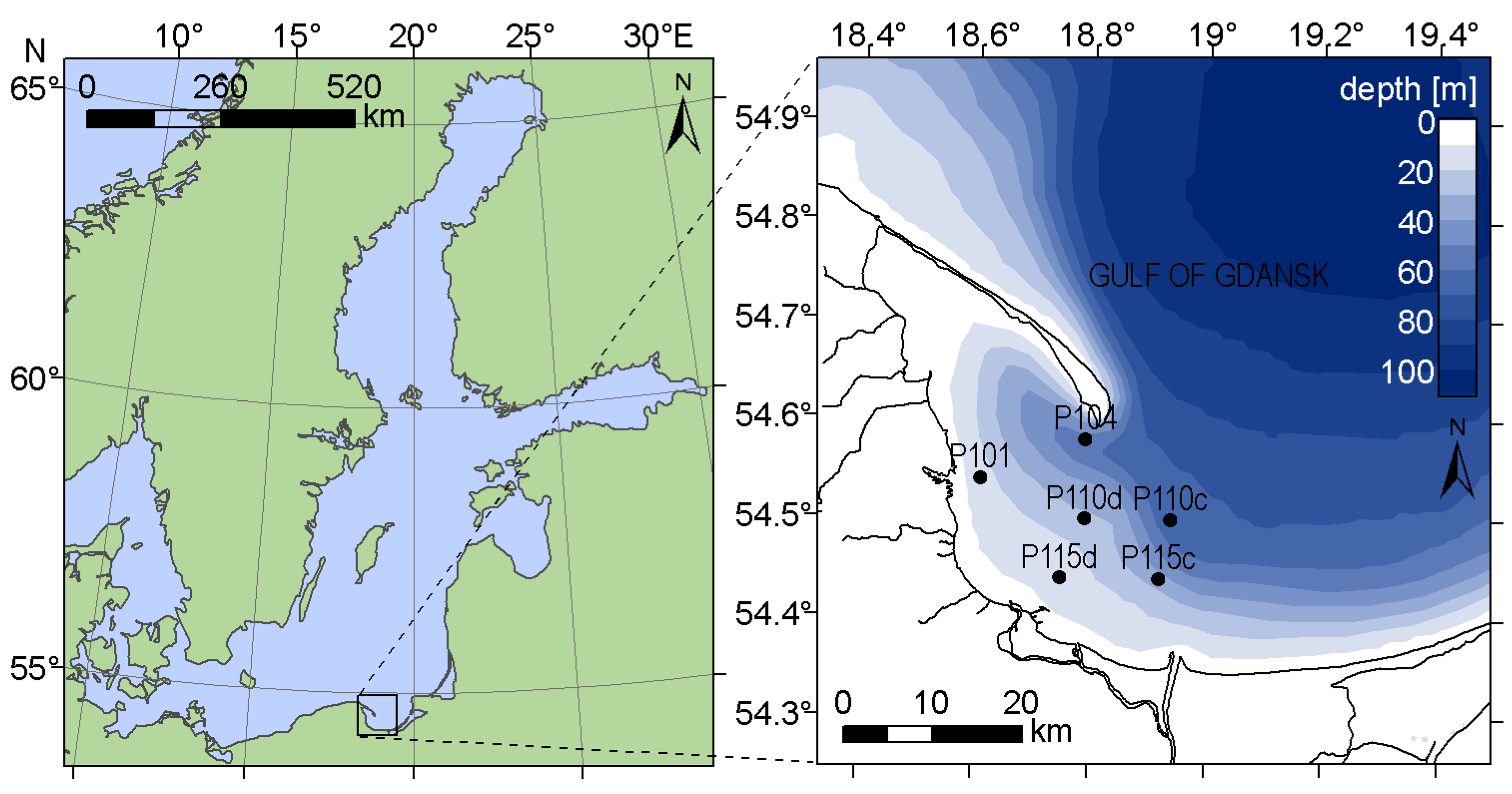
Experimental data were collected during nineteen field campaigns in the late springs and summers of 2012 and 2013 in the western part of the Gulf of Gdansk, southern Baltic Sea (Figure 1). Field campaigns consisted of cruises with the research vessel Oceanograf−2, during which radiometric parameters were measured to retrieve the remote sensing reflectance Rrs, and water samples were taken for laboratory analysis of pigment concentration and other parameters related to the optical properties of water (absorption coefficient of CDOM at 400 nm, Secchi depth and number of phytoplankton cells) using standard methods (described in [32]).
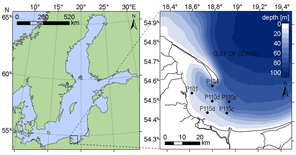
Figure 1.
Spatial distribution of sample stations in the Gulf of Gdansk, Baltic Sea.
The Gulf of Gdansk is a Case 2 water [22], characterized by wide ranges of non-covarying suspended particulate matter (SPM), CDOM and phytoplankton concentrations. The total absorption coefficient, especially for short wavelengths, is dominated by detritus and CDOM absorption, which causes a shift of the absorption minimum towards the red part of the spectra, sometimes even close to 600 nm [33]. These properties affect the shape of the remote sensing reflectance spectra by shifting the maximum towards longer wavelengths, as compared with the Rrs spectra in Case 1 waters [25]. The studied area is a wide and relatively shallow water body, connected with the open sea and strongly influenced by riverine waters (Figure 1). It features many different hydro-geomorphological regimes, including lagoons, river mouths, and sheltered and open coastal areas, and it experiences strong anthropogenic pressure [34]. In the Gulf of Gdansk, the vegetation season usually starts with the bloom of diatoms and dinoflagellates in late March [35]. Cyanobacteria species able to fix atmospheric nitrogen start to dominate in summer, when dissolved nitrogen resources decrease and water temperature is the highest. During the same period, dinoflagellates or green algae can still dominate blooms in regions with higher inflow of nutrients from land. Summer algal blooms in the Gulf of Gdansk are dominated by cyanobacteria [32,35], primarily by the two filamentous, nitrogen-fixing species: Nodularia spumigena and Aphanizomenon flos−aquae [36]. Dolichospermum spp. also occurs in the summer algal blooms, but it is not the dominating species [37]. All these species are rich in phycocyanin [8].
Research cruises usually take place twice per month in May and September (depending on weather conditions), and up to four times per month in June, July and August, when the likelihood of cyanobacteria bloom is the highest [35]. In total, 71 datasets were collected. Measurements were taken between 7:00 a.m. and 1:00 p.m. UTC (9:00 a.m. and 3:00 p.m. local time), which corresponds to solar elevation between 34 and 57 degree. Samples were taken at maximum six locations in the area between 18.4°E−20.0°E and 54.2°N−54.8°N (Figure 1), chosen to cover the wide diversity of hydrological, hydrochemical and optical properties in these waters. The stations P101, P110d and P115d are located in the western, shallow-water part of the Gulf of Gdansk, characterized by relatively high concentration of dissolved phosphate, associated with the municipal and industrial sewage discharged into the Gulf of Gdansk from urbanized coastal area [34]. During favorable wind direction (S, dominating in autumn-winter season), P115c and P110c can be under the influence of Vistula river inflow, which is usually associated with high content of CDOM, suspended matter and nutrients such as silicate, nitrate, nitrite and ammonia. This part of the Gulf is also characterized by lower salinity. However, in the case of the prevailing northeastwards Vistula flow (winds W, SW and NW), the concentration of optically significant constituents at these stations decreases. The northernmost station P104 can be influenced by both, the less transparent waters of the Gulf and the inflow of relatively clear waters from the open sea, coming from the northern side of the Hel Peninsula, where coastal upwellings often occur.
2.2. Radiometric Measurements
Upwelling radiance Lu(0−,λ) (W·m−2·nm−1·sr−1) just below the water surface was measured using the RAMSES−MRC TriOS hyperspectral radiance sensor. This radiometer is characterized by narrow detector and in-air nominal full-angle field-of-view of 20°, which helps to minimize the self-shading error during measurements. At the same time, downwelling irradiance Ed(0+,λ) (W·m−2·nm−1) above the water was measured using RAMSES−ACC−VIS TriOS hyperspectral irradiance sensor. In order to calculate the remote sensing reflectance, the upwelling radiance measured below the water surface Lu(0−,λ) was transferred into the air medium Lu(0+,λ) using the standard procedure, i.e., by applying the immersion factor If [38,39]. On the basis of the received spectra, the remote sensing reflectance Rrs(0+,λ) was calculated using equation:
Although hyperspectral radiometers, such as RAMSES TriOS are becoming increasingly popular in field measurements, satellite remote sensing still relies on multispectral radiometers. In order to explore the feasibility of the developed models with multispectral data available for satellite radiometers such as MERIS (Envisat) or OLCI (Sentinel-3), synthetic satellite data (RrsOLCI) were created from the hyperspectral Rrs data measured from the research vessel by averaging the data around the waveband centers used by the OLCI radiometer between 400 and 800 nm (400 nm, 412.5 nm, 442.5 nm, 490 nm, 510 nm, 560 nm, 620 nm, 665 nm, 673.75 nm, 681.25 nm, 708.75 nm, 753.75 nm, 761.25 nm, 764.375 nm, 767.5 nm, and 778.75 nm). A Gaussian curve was defined with a full width half maximum (FWHM) of the corresponding bandwidths and this was used to weigh Rrs values on either side of the band center during averaging.
2.3. Phycocyanin Measurement
During radiometric measurements, surface water samples were also collected, filtered through Whatman GF/F filters, and frozen until analysis. For each water sample, three filters were prepared for later analysis and the results were averaged to minimize the error. Phycocyanin concentrations were determined in Marine Biophysics Laboratory (Institute of Oceanology, Polish Academy of Science) with the spectroscopic method described in [8]. The mean accuracy of pigment measurement from water samples is 9.71% ± 6.44% (J. Stoń-Egiert, personal communication, 1 February 2016).
2.4. Model Development
The use of Rrs band ratio instead of singular Rrs bands is popular in remote sensing models. The reflectance of a singular band can be influenced by more than one component, whereas the use of band ratios gives enhanced spectral signatures of different water constituents and reduced illumination effects. It is also less sensitive to the atmospheric correction errors when applied to satellite data.
In aquatic environments, parameters such as pigment concentrations are usually log-normally distributed [40]. In [23] it was shown that models for chl−a concentration based on the logarithmic transformation of band ratios performed better for the waters of the Baltic Sea than their linear versions. Similarly, PC concentration appears to be log-normally distributed, and therefore logarithmic transformation has been applied to PC concentration.
The above-mentioned considerations resulted in the following model:
where PC is phycocyanin concentration, k and l are the best fit coefficients, , and Rrs (λi) and Rrs (λj) are the remote sensing reflectance at wavelengths λi and λj, respectively.
In order to find the band ratio with the maximal sensitivity to changes in PC concentration in the studied area, all band ratio combinations in the spectral range between 400 nm and 750 nm and with intervals of 5 nm were examined. This resulted in 5041 band ratios, which thereafter were used to estimate PC concentration using regression analysis and Equation (2).
Regression results were studied by both visual inspection of scatter plots and examination of the determination coefficient R2 and root-mean-square error (RMSE). The ten best band ratios were selected for further analysis.
We assume that estimation performance can be improved using a linear combination of few pre-selected band ratios. Linear combination of correlated variables results in a decreased significance of the corresponding regression parameters. Thus, in the next step, intercorrelation of the ten pre-selected band ratios was studied. In order to avoid overfitting from each group of highly correlated terms (|r| > 0.95, which means R2 > 0.9), only the most physically meaningful terms were selected.
The described procedures resulted in a set of band ratios that were used in the following multilinear model:
where M is the total number of selected band ratios, and , and k and lm are the best fit coefficients.
The aforementioned analysis was performed for hyperspectral data (“PChyp“ model). Next, the model was adapted to the multispectral case (“PCOLCI“ model) by selecting the nearest available OLCI bands. Then, multilinear regression was used to estimate model parameters. Both versions of the models were evaluated separately but in the same manner.
To show the potential usefulness of PCOLCI in case of phytoplankton blooms in the Baltic Sea, data registered by MERIS (Envisat) radiometer were used as an example. All spectral bands of the MERIS radiometer will also be available in the OLCI radiometer on-board the Sentinel-3 satellite, so the model PCOLCI can be used with the data acquired with both radiometers. Remote sensing reflectances from MERIS data, atmospherically corrected using the Case−2 Regional (C2R) processor [41] recommended for Case 2 waters, were used to estimate PC and chl−a concentration. Chl−a concentration was calculated with equation Ca(0)MD proposed in the DESAMBEM project (Equation AIII.3 in [42,43]) and evaluated as the most accurate model for chl−a surface concentration in the Baltic Sea [44]. The PC concentration was calculated with PCOLCI (described further in Section 3.4.2).
2.5. Model Assessment
Since the models presented in this paper were developed in log10 space, all statistics reported are based on log10 transformed data [21,40]. These statistics are determination coefficient R2, systematic error (bias, log10 (mg·m−3)), and statistical error in terms of root-mean-square error (RMSE, log10 (mg·m−3)). Bias and RMSE were calculated using equations:
where is the ith observation, is ith modeled value, and N is the total number of compared pairs.
These statistics quantify regression results for log-normally distributed variables, which are often observed for the datasets like pigments concentration or number of phytoplankton cells. RMSE error was also normalized to the range of observed values (in log10 space) and expressed in percent:
where is the maximal observed value, and is the minimal observed value.
The units of both bias and RMSE are in decades of log10 space and not easily translated into absolute terms. Therefore, following [45,46], we calculated a dimensionless inverse transformed value for bias using:
Thus, Fmed is the median value of ratio /. For instance if Fmed is 1, there is no model bias, if Fmed is 2, the model overestimates by a factor of 2; if Fmed is 0.5, the model underestimates by factor of 2. Median percent difference (MPD), a relative error was calculated using the formula:
Models were built using all data points (N = 71). Collected dataset showed a variety of PC concentration as well as its ratio to chl−a concentration and other optically significant components (see Section 3.1). The dataset covers many common situations in the Baltic Sea coastal waters but it is not big enough to split it into fixed training and validation subsets. Therefore, the presented model errors characterize the residuals, not the prediction performance.
To confirm the robustness of the models, cross-validation was performed for each model. The data were split into training and validation sets. Model parameters and R2 were estimated using 70%, randomly chosen observations, using the MATLAB function randsample. The remaining 30% observations were used for validation, i.e., estimation of prediction bias and RMSE. Randsample function selects each data point with equal probability, and it is therefore expected that the test data typically included points spread uniformly in time. This makes it unlikely that the training dataset consisted entirely of points from one season. The procedure of randomly selecting training and validation subsets was repeated 5000 times to capture the distribution of the prediction errors, both in terms of the mean and standard deviation. For a robust and generalizable to other datasets model, cross-validation model skill should be reduced only slightly compared with the model derived from the full dataset.
3. Results and Discussion
3.1. Field Measurements
During field measurements, water transparency by means of Secchi depth varied between 1.5 m and 7 m and CDOM absorption (at 400 nm) varied between 0.72 m−1 and 2.1 m−1 (Table 1). In terms of the total number of phytoplankton cells, cyanobacteria contributed to at least 50% from the middle of June until the end of August [32,35]. The chl−a concentration measured in the Gulf of Gdansk varied between 0.93 mg·m−3 and 30.91 mg·m−3 (in log10 space: −0.03 and 1.49, respectively), with a mean value of 7.3 mg·m−3 (0.71 in log10 space) and a median value of 4.6 mg·m−3 (0.66 in log10 space), see Figure 2. The measured values are in the range of chl−a concentration typical for the southern Baltic Sea with skewed distribution, where most values are low and around 2−3 mg·m−3, while high chl−a concentrations, even up to 100 mg·m−3, can occur during algal blooms [23,36]. Due to the occurrence of upwellings, riverine inflows, and the effect of algal blooms, the water composition in the Gulf of Gdansk shows high variability, which can cover the typical situation for the whole Baltic Sea waters.

Table 1.
Water transparency (Secchi depth) during sampling and statistical characteristics of environmental parameters measured in the same water samples: aCDOM(400 nm): CDOM absorption at 400 nm, PC: phycocyanin concentration, chl−a: chlorophyll a concentration, PC/chl−a: ratio of phycocyanin to chlorophyll a concentration, phytoplankton biomass, cyanobacteria biomass content: content of cyanobacteria in total mass of phytoplankton, phytoplankton cells number, cyanobacteria cells content: content of cyanobacteria cells in total number of phytoplankton cells. Min.: minimum, Max.: maximum values; Q: quantiles.
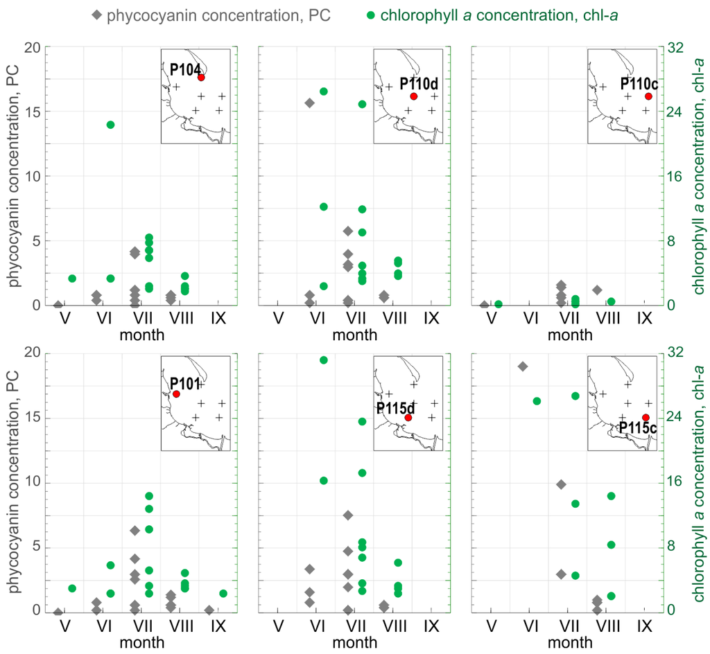
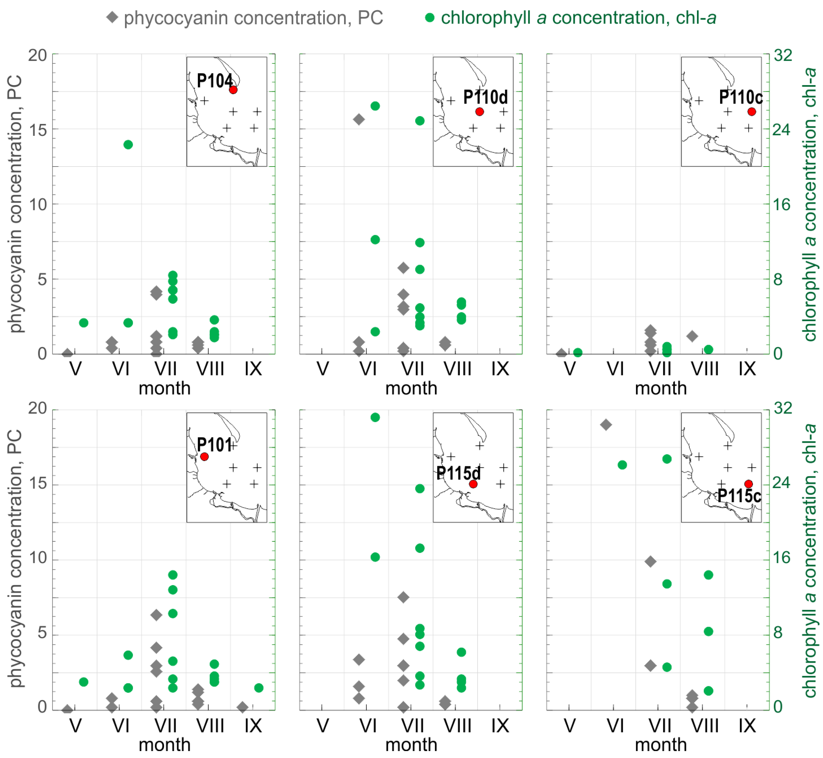
Figure 2.
Spatial and temporal distribution of PC (left axis, gray) and chl−a (right axis, green) measured during our studies (in mg·m−3). The same scale is used for each type of axis in all six diagrams. Red points on simplified maps show location of sampling stations in relation to the coastline and rivers.
PC concentration varied during the same period from 0.05 mg·m−3 to 18.95 mg·m−3 (in log10 space: −1.29 and 1.28, respectively), with a mean value of 2.14 mg·m−3 (0.02 in log10 space) and a median value of 0.84 mg·m−3 (−0.07 in log10 space), see Figure 2. The minimal value was observed at the beginning of May, when the taxonomic composition of phytoplankton is typically dominated by diatoms and dinoflagellates, whereas the maximal value of PC concentration was observed in the last week of June, when cyanobacteria species typically start to dominate the phytoplankton composition [35].
Data collected in June at stations P104 and P115d show typical situation for the waters of the Gulf of Gdansk during early summer (Figure 2). During that time, the concentration of nutrients is still high, which promotes and supports the growth of dinoflagellates and green algae. Chlorophyll concentration was over 10 mg·m−3 and concentration of phycocyanin was generally below 2.5 mg·m−3, which indicated relatively high biomass of phytoplankton but low contribution of cyanobacteria. In the later summer, when dissolved nitrogen resources decrease, cyanobacteria species able to fix atmospheric nitrogen start to dominate. For the same reason, the regions located further from the nutrient sources are more affected by cyanobacteria blooms. In such situation, high concentration of chlorophyll is expected to be accompanied by high concentration of phycocyanin, as observed in June at P110d and P115c (chl−a > 25 mg·m−3, PC > 15 mg·m−3). Samples from station P110c from each cruise represented waters relatively poor in phytoplankton (Figure 2).
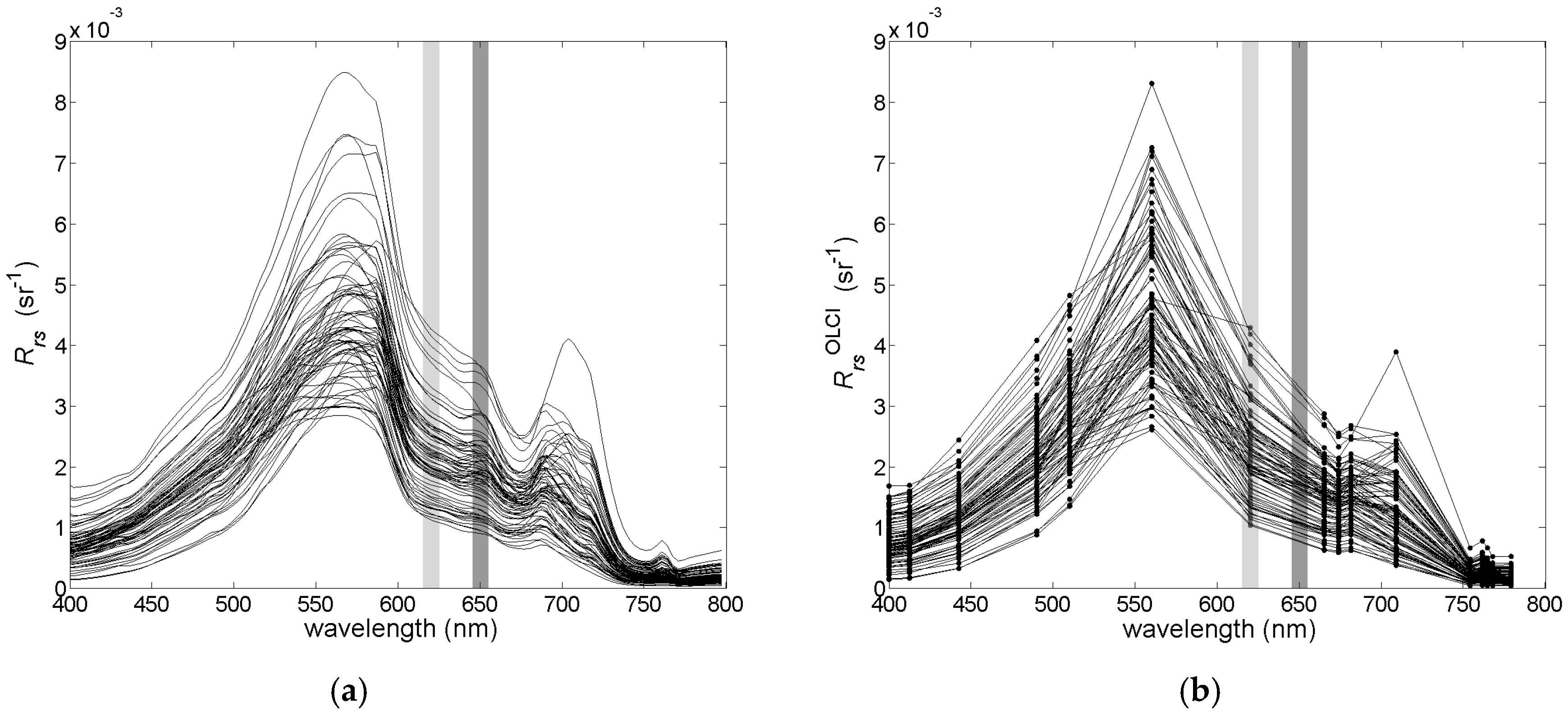
Variability of the optically significant water components influences the shape and magnitude of remote sensing reflectance (Rrs) spectra collected in the field campaigns (Figure 3a). The collected Rrs spectra represent quite typical spectral features consistent within optically complex waters [25]. The maximal value of Rrs is found between 550 nm and 560 nm, and it shifts into the longer wavelength with increasing magnitude of the reflectance. There is a strong decrease and a small variability of the Rrs values in the blue part of the spectrum due to high absorption of yellow substances and detritus in the studied area. The local minimum, near 660 nm, and the maximum, near 680 nm, correspond to the maximal absorption and fluorescence, respectively, of chl−a. In Figure 3a,b, two spectral bands are highlighted, one around 620 nm, where the maximal absorption of phycocyanin is observed, and one around 650 nm, where the maximum fluorescence of phycocyanin is observed. These features are clearly visible in the hyperspectral data in Figure 3a, but after converting the hyperspectral Rrs data to the multispectral cases of the MERIS and OLCI sensors, they become less distinct (Figure 3b).

Figure 3.
The variance of the studied Rrs spectra for the (a) hyperspectral and (b) multispectral cases. Narrow spectral bands around the maximum of absorption and fluorescence of phycocyanin are highlighted in light and dark grey, respectively.
3.2. Assessment of Known Models
Several empirical or semi-empirical models for phycocyanin estimation with remote sensing methods have been published in the past [10,11,13,15,31,47]. The models use different predictors, mostly a combination of Rrs measured for different wavelengths, but also inherent optical properties. However, none of the models are developed to Baltic Sea waters. In our studies, we have examined the predictors used in those of the published models, which only use Rrs spectra for PC concentration estimation, without any prior knowledge of inherent optical properties. Each one of the predictors summarized in Table 2 was used to estimate PC concentration for our dataset. The following linear model was used:
where XREF is one of the predictors summarized in Table 2, and k and l are model parameters, estimated using linear regression.
Table 2.
A summary of the predictors used in some previous studies.
In general, PC estimation using Equation (9) and the predictors summarized in Table 2 showed very poor results, in all cases with R2 below 0.5 and RMSE higher than 0.4. One major reason for the poor performance may be differences in the used data. The predictors in Table 2 were selected for datasets with PC concentration much higher than in the Baltic Sea waters. For example, the average value of PC was 419 mg·m−3 in [48] and 68.9 mg·m−3 in [31], whereas for the Gulf of Gdansk, it was 2.14 mg·m−3, and the maximum was 18.95 mg·m−3.
Typically, PC concentration is characterized by a log-normal distribution [40]. Following the form of the models for chl−a concentration, which has the same distribution in the waters of Baltic Sea [23], Equation (9) was modified to the form of Equation (2), where variable XREF was used in place of X. The use of logarithms instead of linear values improved the results. The greatest improvement was noted for SY00 and SP05, resulting in R2 = 0.66, and RMSE = 0.29 for SY00 and R2 = 0.63, and RMSE = 0.31 for SP05. MM09 and MS12 also showed significant improvement of R2 to around 0.6 and RMSE to around 0.33, while the results for DA93 and HP10 were still poor, with R2 below 0.3 and RMSE around 0.4. This analysis gave us motivation and suggestions for further model development for our study area.
3.3. Optimal Band Ratio Selection
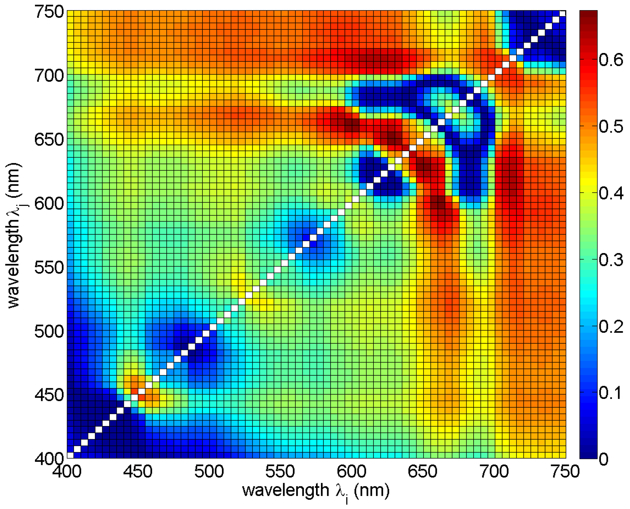
In the first analysis, the correlation between single band ratios and phycocyanin concentrations was studied by fitting Equation (2) to the reference data for all band ratios in the range between 400 nm and 750 nm, with a step of 5 nm. The scatter plots (not shown) and the values of determination coefficients R2 (Figure 4) were studied. It was observed that band ratios involving data from the two spectral ranges 640−660 nm and 600−620 nm show the highest R2 values, over 0.6. Meanwhile, the values of R2 for the band ratios commonly used in optical remote sensing methods (e.g., 440/555, 490/555 or 510/555) were low, around 0.3.
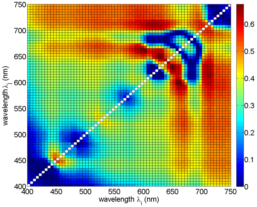
Figure 4.
Determination coefficient R2 for Equation (2) for all possible band ratios Rrs(λi)/Rrs(λj) in the spectral range 400–750 nm.
The wavelengths for the best ten band ratios (all with RMSE < 0.3, R2 ≥ 0.6, and p-value << 0.0001) are in the spectral range from 590 nm to 710 nm (Table 3 and Figure 4). Normalized RMSE for all chosen band ratios was around 11%, while bias was around 0 (Fmed was around 1), so on average the model was unbiased. The relative error MPD was around 45% for most of the models, with a minimum of 40% (for model #7) and a maximum of 59% (for model #1). In this spectral range, Rrs values are influenced by absorption and fluorescence of phycocyanin and chlorophyll a, whereas the absorption of yellow substances has minimal effect on the Rrs [49]. This is important in the waters of the Baltic Sea, where CDOM dominates the total absorption coefficient in the blue and green part of the spectrum [25,50]. For most of the ten chosen band ratios, the values of phycocyanin concentration decrease with increasing value of reflectance ratio (coefficient l < 0), see Table 3.
Table 3.
Estimated coefficients and basic regression statistics for the ten best band ratios used with one-term model (Equation (2)).
The best results of fitting of the single band ratio model (Equation (2)) were achieved for the band ratio (595/660), see Figure 5, which represents the fraction of the minimal absorption coefficient of the optically significant components in Baltic Sea waters [49] to the maximal absorption of chl−a. Therefore, it has a certain physical explanation and can be selected for further consideration within the multilinear model (Equation (3)). Another three pre-selected band ratios (#3, #6 and #7 in Table 3) are highly correlated with band ratio #1 (Table 4). A linear combination of such variables results in a decreased significance of the corresponding regression parameters, and they were therefore rejected from further considerations.
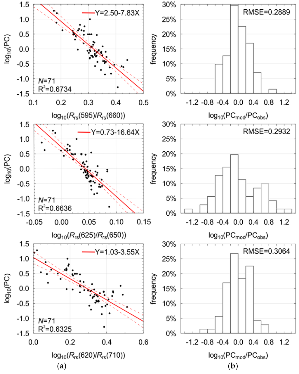
Figure 5.
The dependence between the logarithm of PC concentration and the logarithm of the selected remote sensing reflectance band ratio (a) and distribution of the regression residuals (b). Also shown are: regression line with 95% confidence interval, best fit coefficients, the number of observations (N), the coefficient of determination (R2), and the root-mean-square error (RMSE).
Table 4.
Correlation matrix for logarithmic transformation of the ten best band ratios used with one-term model (Equation (2)). #x is a number of model from Table 3; correlation coefficients over 0.95 are highlighted (all correlations are statistically significant at the p-level < 0.01).
From the rest of pre-selected band ratios, those for which the coefficient l shows the highest absolute values (#2, #4, and #5 in Table 3) seem to be the most sensitive for estimation of PC concentration. However, their values are 2−3 times lower than these discussed above. The intercorrelatation between them is also very high (Table 4). These three band ratios make use of wavelengths around 625 nm and 650 nm, which are the closest to the absorption and fluorescence maxima for phycocyanin [8,51]. Taking into account the optical properties of PC, the Rrs spectrum close to 650 nm has stronger correlation with fluorescence of phycocyanin than 645 nm [8], while 625 nm has stronger correlation with absorption of phycocyanin than 630 nm [51]. Thus, as the second variable for further analysis, band ratio (625/650) was chosen. Studies presented by Schalles and Yacobi [47] also show the usefulness of this band ratio. The remaining three of the ten pre-selected band ratios use the band 710 nm, where the absorption coefficient is strongly dominated by water particles and the magnitude of Rrs is increasing together with suspended particulate matter concentration. Thus, in the model created for Case 2 waters, where the magnitude of Rrs spectra is increasing together with the concentration of suspended particulate matter due to high scattering, the inclusion of bands from the far red is reasonable and could help to minimize influence of suspended particles on model results. Taking into account their very high intercorrelation, only band ratio (620/710) was selected for the multilinear regression, as it also incorporates band of the maximal absorption of phycocyanin (620 nm), whereas in the range of 610−615 nm the optical properties of water in the Baltic Sea do not show any other characteristic features. Simis et al. [13] also used a similar band ratio in their semi-empirical model. All band ratios selected for multilinear model (Equation (3)) in relation to the phycocyanin concentration are shown in Figure 5.
3.4. Multilinear Model for PC Estimation
3.4.1. Hyperspectral Data
The three selected band ratios (Figure 5) were used as phycocycanin predictors in the multilinear model (Equation (3)), further briefly referred to as PC3term, with , , , and the regression coefficients were estimated by fitting model to the data using multilinear regression (Table 5). The three-term model allows PC estimation with RMSE = 0.26 (NRMSE = 10%), MPD = 39% and R2 = 0.74 (adjusted R2 = 0.73, ANOVA statistic F = 63.19, significance level p-value << 0.0001, standard error of estimation: 0.27). Results of regression (Figure 6a,b) show improvement compared with the models with only one band ratio (Figure 5). For 73% of the cases, residuals of regression were in the range of ±0.26 (RMSE in log10 space). This means that the three-term model biases the estimated PC by a factor between 0.55 and 1.82 in the most cases. Such range of residuals for single band ratio models were observed for less than 65% of cases.
Table 5.
Statistical characteristics of multilinear regression coefficients for multilinear model shown in Equation (3) utilizing three or two predictors (coefficients marked by * refer to factors after standardization).
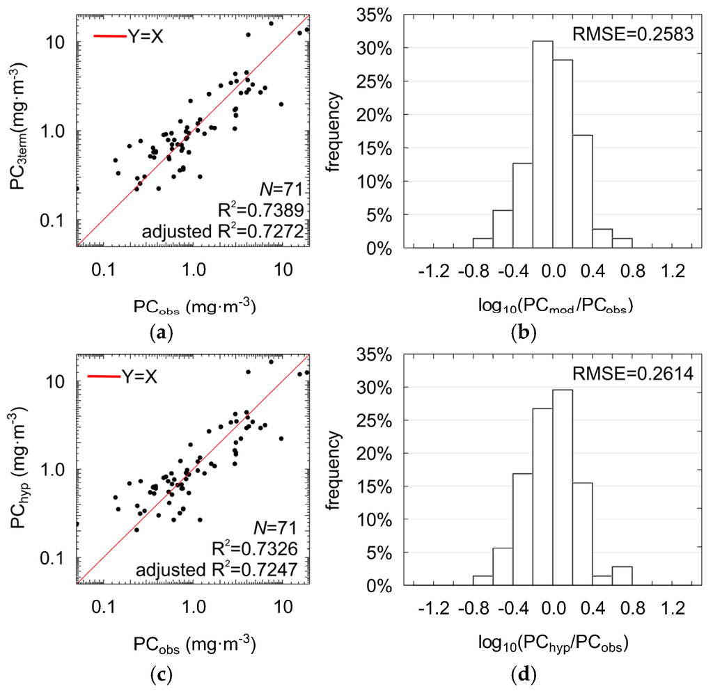
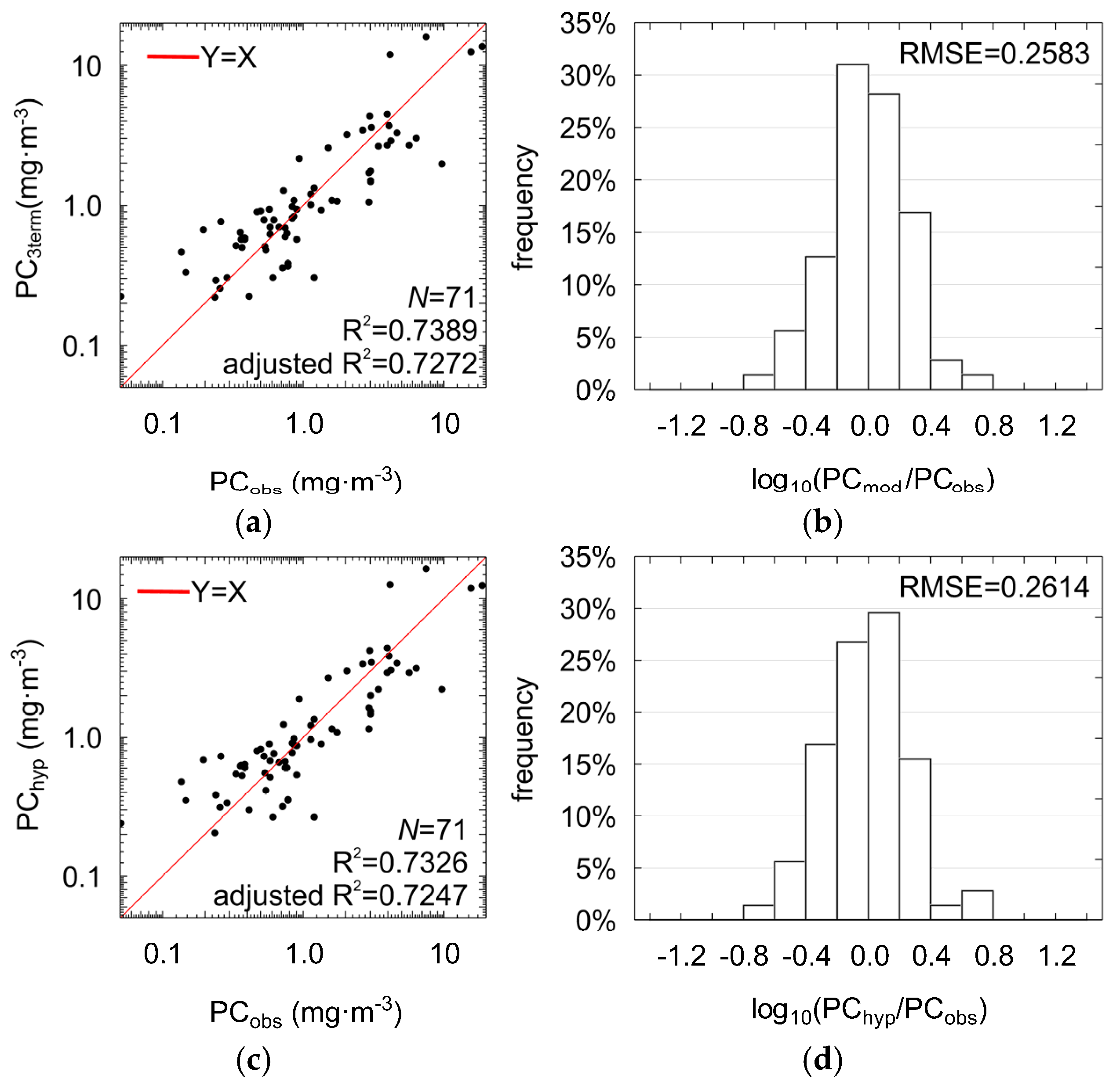
Figure 6.
Scatter plots showing comparison between the PC concentrations measured in situ and estimated using the three-term model (PC3term) shown in Equation (3) with: X1 = Rrs(595)/Rrs(660), X2 = Rrs(625)/Rrs(650), X3 = Rrs(620)/Rrs(710) (a); distribution of the PC3term regression residuals (b); two-term model (PChyp) with: X1 = Rrs(625)/Rrs(650), X2 = Rrs(620)/Rrs(710) (c); and distribution of the PChyp regression residuals (d).
The core part of the multilinear three-term model (PC3term) is the component Rrs(625)/Rrs(650), which consists of a reflectance ratio for wavebands with the maximal absorption (625 nm) and maximal fluorescence (650 nm) of light by phycocyanin. Values of this band ratio vary in a relatively narrow range (Figure 5). However, the corresponding coefficient has an absolute value large enough to make the model sensitive to even small changes in the shape of Rrs at this part of spectrum, reflecting changes in PC concentration, see Table 5. Similarly high contribution to PC estimation is given by the band ratio (620/710). The first term (595/660), despite its highest correlation with PC, is the least significant (p-value close to 0.2). Moreover, it is highly correlated with the two other band ratios (Table 4), which increases the risk of overfitting. Although the removal of the least significant band ratio gives a model with somewhat worse performance (R2 = 0.73, adjusted R2 = 0.72, RMSE = 0.2614, NRMSE = 10%, MPD = 38%), we chose to use the two-term model in the subsequent analysis, further briefly referred to as PChyp (Table 5, Figure 6c,d):
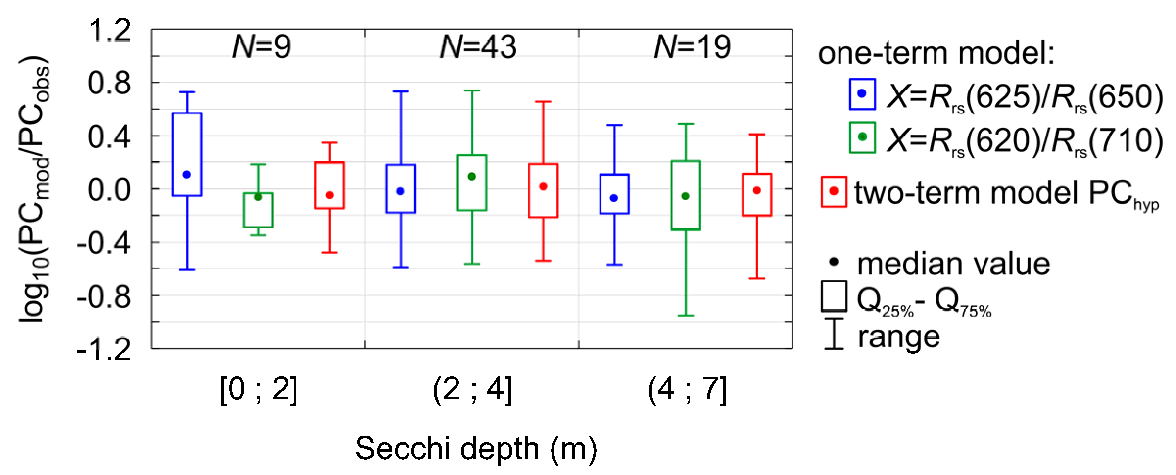
where , (ANOVA statistic F = 93.15, significance level p-value << 0.0001, standard error of estimation 0.27). This combination of two components gives somewhat narrower distribution of residuals (Figure 6d) in comparison to the one-term models (Figure 5) and, what is more important, PChyp model seems to be more stable in different conditions of water transparency (Figure 7). In the Baltic Sea, during cyanobacterial blooms Secchi depth can decrease to less than 4 m in the open sea and even to less than 2 m in coastal areas [52]. The coastal area is more problematic since the input of nutrients from rivers promotes and supports the growth of other phytoplankton groups, i.e., dinoflagellates and green algae. Thus, relatively high biomass of phytoplankton and chlorophyll a concentration occurs together with low contribution of cyanobacteria. In water with such low transparency, the one-term model overestimates PC if X = Rrs(625)/Rrs(650) and underestimated if X = Rrs(620)/Rrs(710) (Figure 7).

Figure 7.
Distribution of regression residuals for different PC models (two one-term models according to Equation (2) and one two-term model PChyp according to Equation (10)) for different water transparency conditions (Secchi depth as an indicator for transparency).
3.4.2. Multispectral Data
When multispectral data with bands characteristic for MERIS and OLCI radiometers are considered, model PChyp (Equation (10)) can be adapted by using the nearest bands available for these spaceborne sensors, further briefly referred to as PCOLCI:
where , the best fit coefficients are given in Table 6.
Table 6.
Statistical characteristics of multilinear regression coefficients for PCOLCI model shown in Equation (11) (coefficients marked by * refers to factors after standardization).
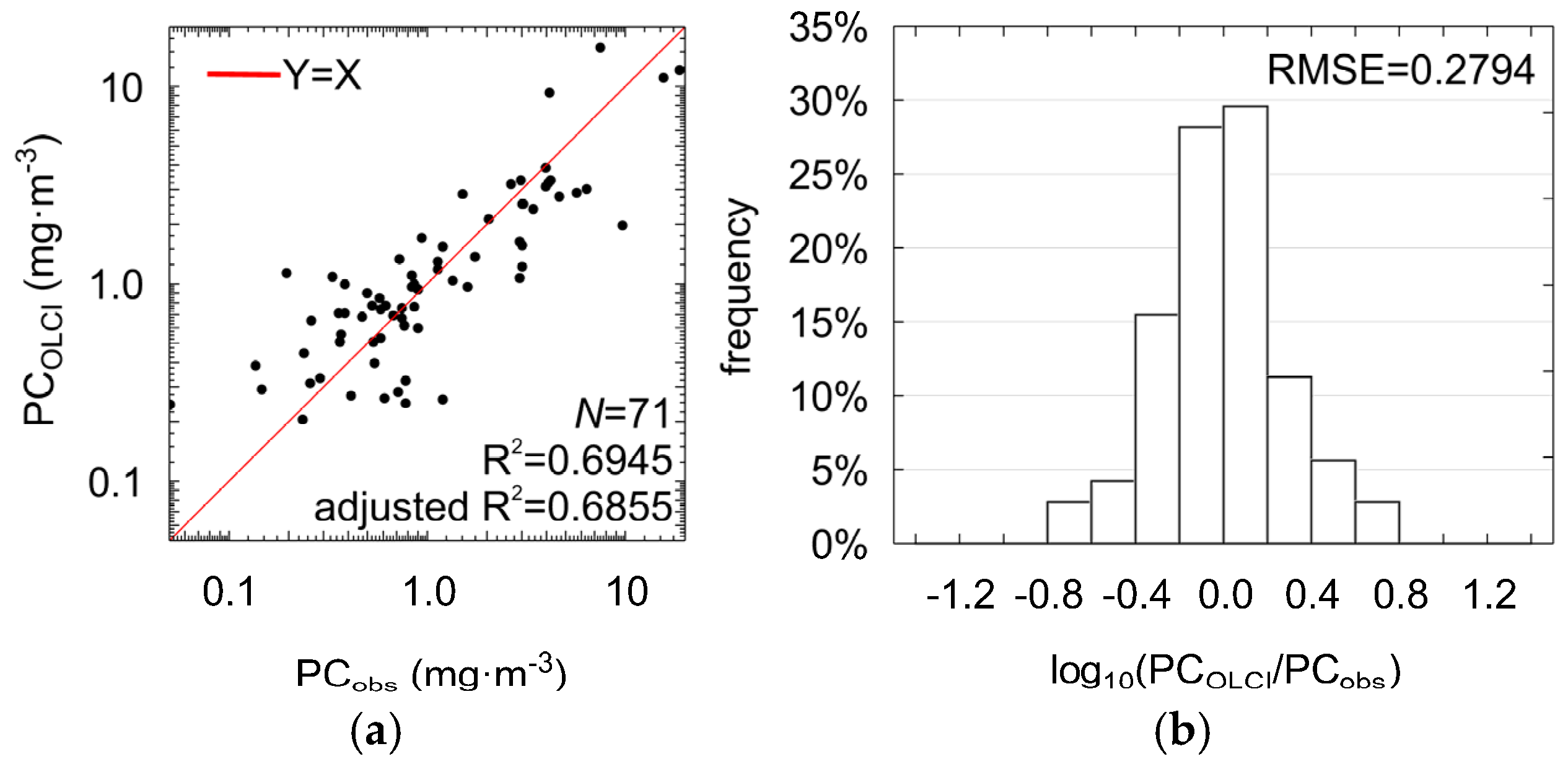
This modification did not significantly influence the accuracy of estimation of PC concentration (R2 = 0.69, adjusted R2 = 0.69, RMSE = 0.28, MPD = 37% NRMSE = 11%, ANOVA statistic F = 77.31, significance level p-value << 0.0001, standard error of estimation = 0.29, see Figure 8 and Table 6). For 70% of the cases, residuals of regression were in the range of ±0.28 (RMSE in log10 space). This means that the estimated PC can be higher or lower in relation to measured value by a factor between 0.52 and 1.91. Therefore, PCOLCI (Equation (11)) can be used together with data acquired with the previous satellite radiometer MERIS, as well as the OLCI radiometer onboard the Sentinel-3 satellite, to monitor large-scale changes in PC concentration in the surface waters.
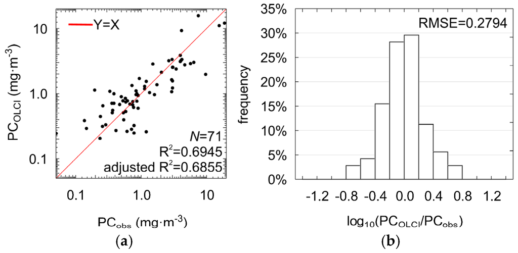
Figure 8.
Scatter plots showing the correlation between the PC concentrations measured in situ and estimated using the PCOLCI model shown in Equation (11) (a) and distribution of the regression residuals (b).
Figure 9 shows sample maps of PC concentrations derived from data registered by MERIS (Envisat) radiometer on three different occasions, together with maps of chl−a and RGB images of the Baltic Sea. In April (Figure 9a), high chl−a concentration (up to 17 mg·m−3 in the eastern part of the sea) explains green patches which can be seen on RGB composite. However, temperature in spring is too low to trigger cyanobacteria bloom; instead, other species form the bloom. Therefore, phycocyanin concentration is expected to be below, or close to the limit of detection. Estimation using PCOLCI provides phycocyanin concentration less than 1 mg·m−3 in the whole Baltic Sea, which is within the margin of the estimation error of this model.
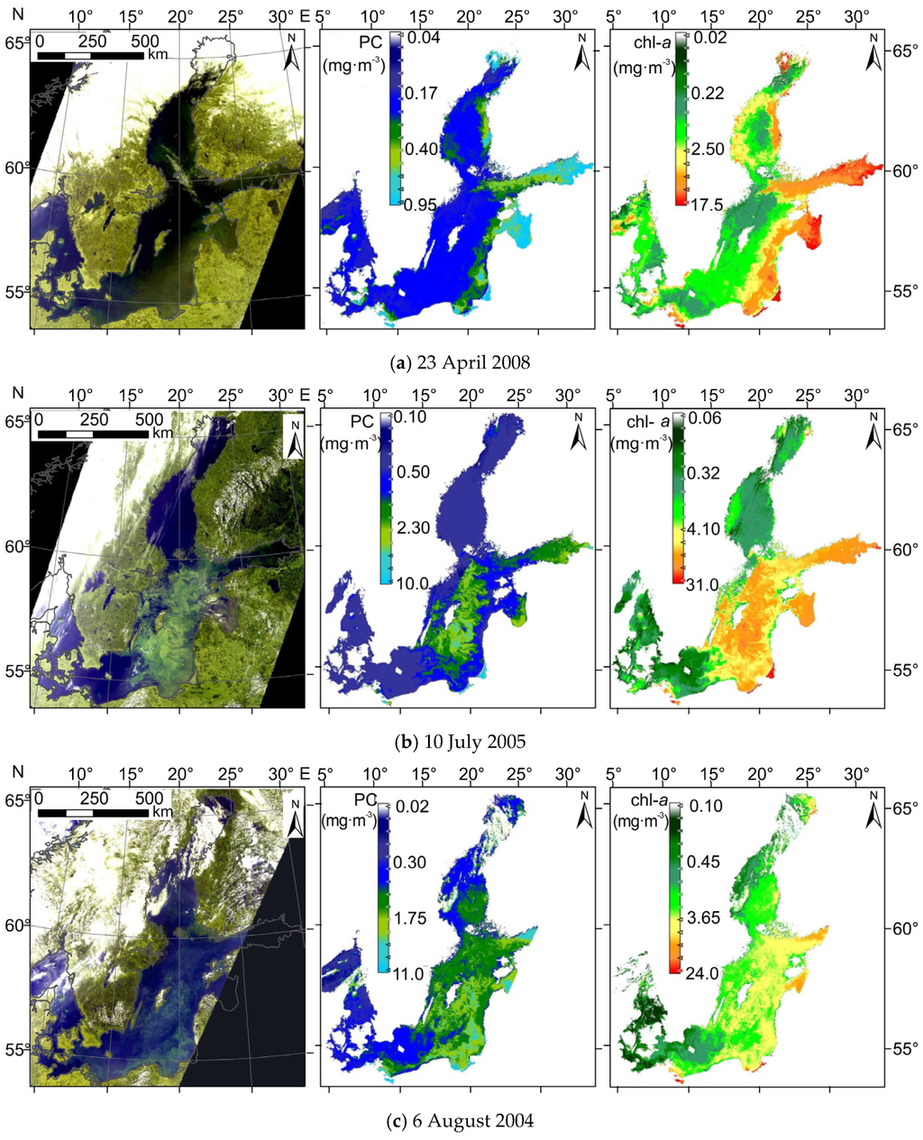
Figure 9.
(Left) RGB image; (center) spatial distribution of PC concentration; and (right) spatial distribution of chl−a concentration for sample scenes from spring (a) and summer (b,c), recorded during blooms of different phytoplankton composition. Satellite data were acquired by the MERIS sensor onboard the Envisat satellite.
The main advantage of the presented model can clearly be seen on the satellite images acquired during summer, especially in July (Figure 9b), when cyanobacteria blooms usually are observed in the central part of the sea [53]. The differences between the spatial distribution of retrieved chl−a and PC concentration inform whether the phytoplankton biomass is or is not dominated by cyanobacteria. Maps derived from the MERIS data show that in the central area of the sea, there are many regions with high concentrations of both chl−a and PC, whereas this is not observed in the coastal areas. This may suggest that phytoplankton biomass in the coastal area does not contain cyanobacteria species or contains it to a much smaller degree. The opposite situation can be seen on the processed satellite images from August (Figure 9c), where spatial distribution of PC shows similar pattern as chl−a. According to the HELCOM (Helsinki Commission) Baltic Sea Environment Fact Sheets [53,54], in August 2004 phytoplankton composition in the whole Baltic Sea was dominated by cyanobacteria, which has also been confirmed on processed satellite image presented in Figure 9c.
3.5. Model Robustness
The development of models PChyp (Equation (10)) and PCOLCI (Equation (11)) was based on all available data. To evaluate the robustness of the models, cross-validation was used. Table 7 and Figure 10 show the results of cross-validation analysis.
Table 7.
The results of the cross-validation analysis of models PChyp and PCOLCI.
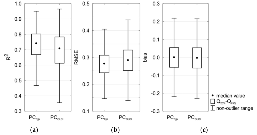
Figure 10.
Box plots showing statistics of: the coefficient of determination (a); RMSE (b); and bias (c) obtained during cross-validation of the selected models.
The mean value of the calculated error statistics (R2, RMSE and bias) in cross-validation analysis did not change significantly compared to the analysis based on the entire dataset, which suggests that both PChyp and PCOLCI seem to be robust and stable. The regression coefficients did not change significantly either. For all statistical metrics, the range of the values from cross-validation was smaller for PChyp than for PCOLCI, except for bias (Figure 10). For both models, average of bias is close to 0.0 (it means Fmed close to 1.0).
3.6. Sensitivity for High chl−a Concentration
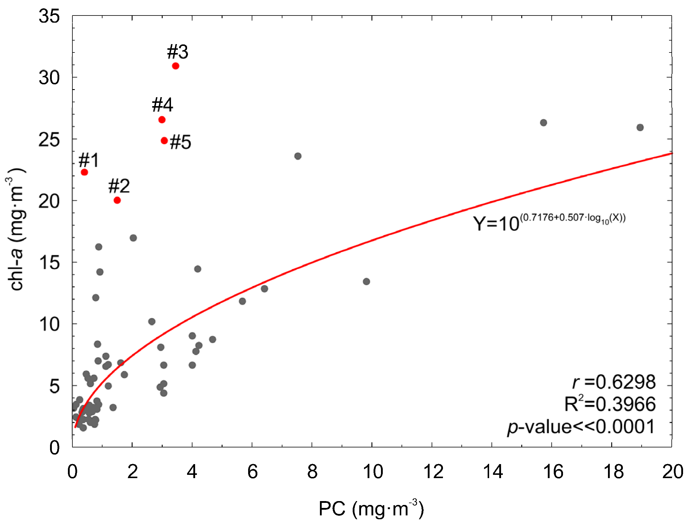
Although it is obvious that chl−a concentration will increase with an increased PC concentration, the opposite does not always occur. When the phytoplankton biomass is high but its taxonomic composition does not contain cyanobacteria species, chl−a concentration can be high while PC concentration is low. Such situation was observed for data from June acquired at stations P104 and P115d (Figure 2 and Figure 11). For these cases, PC concentration was estimated using the PChyp and PCOLCI models in order to verify that the models are robust and not biased by high chl−a concentration. Additionally, PC concentration was estimated from the empirical relation between PC and chl−a, derived from the analyzed dataset (Figure 11):

Figure 11.
PC versus chl−a concentration, both measured in situ. Cases (#1–#5, red dots) when chl−a concentration was high and PC was low, are marked in red.
The results are shown in Table 8. It can be noted that model PChyp is robust and does not overestimate PC concentration when chl−a concentration is high and cyanobacteria biomass is low. This is due to the fact that model PChyp uses the spectral bands related to the maximum of phycocyanin absorption and to fluorescence, which determine the shapes of the reflectance spectra (Figure 3a). In addition, PChyp utilizes band 710 nm, which is outside the range of spectrum influenced by chlorophyll a and other pigments. Such combination makes residuals of PChyp model not correlated with chl-a concentration (correlation coefficient for PChyp residuals vs. log10(chl-a) is r = 0.15, p-value = 0.21). Absolute estimation errors for PCOLCI are similar to the absolute estimation errors for PChyp, but its residuals are slightly correlated with chl-a concentration (correlation coefficient for PCOLCI residuals vs. log10(chl-a) is r = 0.25, p-value = 0.035). This is because the spectral bands of MERIS and OLCI radiometers do not exactly fit to the spectral band responsive to the phycocyanin fluorescence (650 nm) and the nearest channel used in the PCOLCI model was more related to chl−a absorption (665 nm). The model PCOLCI works well for situations when cyanobacteria are dominant (both PC and chl−a concentration are high) but it is less accurate in cases when other species form blooms. It can explain why the spatial distribution of PC concentration evaluated on the basis of MERIS data for April (Figure 9a) shows similar spatial distribution like chl−a concentration.
Table 8.
PC concentration (mg·m−3) calculated using the two models PChyp and PCOLCI for the cases when chl−a concentration (mg·m−3) was high (points #1–#5 highlighted in the Figure 11).
The maps from August (Figure 9c) show also similar spatial distribution of PC and chl−a, however, at this time of year, such correlation is expected and PCOLCI values are more reliable. When different dominating groups of phytoplankton can occur in different regions of the bloom, like in the example from July (Figure 9b), PCOLCI helps to distinguish these regions.
4. Summary and Conclusions
The presented work was focused on the development of a remote sensing reflectance-based model for estimation of phycocyanin concentration (PC) in the optically complex waters of the Baltic Sea. The model has been developed and its robustness confirmed using in situ measurements of reflectance spectra and phycocyanin concentration. The measurements cover the typical range of optical properties that can occur in the Baltic Sea coastal waters. The proposed model is based on linear combination of two variables that are logarithmic transformation of reflectance band ratios. The model has been developed for the optimal spectral bands of reflectance (PChyp version) and later adapted to existing multispectral data from satellite radiometer (PCOLCI version). Depending on version, it uses four (PChyp) or three (PCOLCI) different spectral bands that cover ranges of spectrum related to: the maximal absorption (620–625 nm) and the maximal fluorescence (close to 650 nm) of phycocyanin, and the absorption strongly dominated by water particles where the magnitude of Rrs is increasing together with suspended particulate matter concentration (close to 710 nm).
Despite the challenge of optically complex water with large concentration of CDOM and SPM influencing remotely sensed reflectance spectra in the Baltic Sea, the proposed model estimates the cyanobacteria marker pigment in the Gulf of Gdansk with RMSE values of 0.26 and 0.28, respectively, for the version developed for hyperspectral sensors and the version adapted for the spaceborne, MERIS- and OLCI-type sensors. All spectral bands of the MERIS radiometer will also be available in the OLCI radiometer onboard the Sentinel-3 satellite, so the model PCOLCI can be used with the data acquired from both radiometers. This allows frequent, large-scale monitoring of cyanobacteria biomass, which may find its applications in both climate related research, weather forecasting, coastal management, and risk assessment. Archived MERIS data acquired during its 10 years of operation can also be used in such monitoring for long-term analysis.
Similar empirical or semi-empirical models based on reflectance band ratios have been used in the past [10,11,15,31,47,48]. However, it was shown in this paper that they perform poorly for the waters of the Baltic Sea (RMSE from 0.41 to 0.54) and, even after recalibration using the experimental data used in this paper, the results are poorer than for the model PChyp (Equation (10)) proposed here. The advantage of the presented solution is that it takes into account the statistical distribution of PC concentration characteristic for the Baltic Sea (e.g., through the use of logarithmic transformation). Moreover, it uses a combination of band ratios, which both emphasizes the response of reflectance spectra to changes in phycocyanin concentration and minimizes their response to uncorrelated changes related to other optically significant constituents.
The predictors of PChyp model were chosen based on both statistical analysis and interpretation of physical properties of the selected bands, which makes PC estimation robust and gives an effective tool for monitoring of the occurrence of cyanobacteria filamentous species. As was expected, the best results were achieved using expressions utilizing spectral bands of reflectance determined by the optical properties of phycocyanin (625 and 650 nm). Schalles and Yacobi [47] present a model with a single band ratio (650/625) which is also used in the PChyp model (Equation (10)) proposed in this work. However, as shown in our analysis, the additional (620/710) band ratio of model PChyp increases accuracy and stability of the model, as they also account for the influence of other optically significant components in water. Moreover, in water with low transparency, the one-term models overestimate or underestimate phycocyanin concentration.
The PC3term model showed somewhat better results of estimation than the PChyp model. However, statistical analysis leads us to exclude the band ratio 595/660 as redundant. In the future, additional analysis of a larger dataset from different areas of the Baltic Sea could confirm or totally reject the importance of the 595/660 band ratio.
Comparison of PCOLCI and PChyp models shows that worse performance for PC concentration estimation is obtained if fluorescence of PC is neglected. If replaced by nearest channel of MERIS or OLCI radiometer, results are more dependent on spatial distribution of chl−a concentration, which can be associated with other phytoplankton groups besides cyanobacteria. It suggests the need for new spectral bands in satellite radiometers.
The development of model PChyp was based on Rrs spectra typical for Case 2 waters of the Baltic Sea, which covered wide range of situations. For the other areas, characterized by similar optical properties and similar range of phycocyanin concentration (up to 20 mg·m−3), the model parameters may need to be estimated from reference data. In the future, model PCOLCI also needs to be validated against satellite data and atmospheric corrections should be taken into account in such validation as well.
Acknowledgements
The authors would like to thank Bożena Wojtasiewicz for the participation in field campaigns and laboratory analysis, Joanna Stoń−Egiert and Monika Sobiechowska−Sasim for the laboratory analysis of phycocyanin concentration, as well as Maciej Soja for comments that greatly improved the manuscript. The Project was carried out within the framework of the SatBałtyk project funded by the European Union through European Regional Development Fund (contract No. POIG.01.01.02−22−011/09 entitled “The Satellite Monitoring of the Baltic Sea Environment”) and also as a part of IO UG statutory research (DS/530−G210−D425).
Additionally, the authors would like to thank the anonymous reviewers whose valuable input significantly increased the quality of this paper.
Author Contributions
Monika Woźniak collected the data (radiometric measurements and water sample for laboratory analysis), was involved in the design of the study, analyzed the reflectance spectra, and wrote most of the manuscript. Katarzyna M. Bradtke was involved in the design of the study and contributed with some text and analysis of the reflectance spectra. Miroslaw Darecki and Adam Krężel supervised the work, helped with editing of the manuscript, and provided scientific consultation.
Conflicts of Interest
The authors declare no conflict of interest. The founding sponsors had no role in the design of the study; in the collection, analyses, or interpretation of data; in the writing of the manuscript, and in the decision to publish the results.
References
- Blaha, L.; Babica, P.; Marsalek, B. Toxins produced in cyanobacterial water blooms-toxicity and risks. Interdiscip. Toxicol. 2009, 2, 36–41. [Google Scholar] [CrossRef]
- Landsberg, J.H. The effects of harmful algal blooms on aquatic organisms. Rev. Fish. Sci. 2002, 10, 113–390. [Google Scholar] [CrossRef]
- Boyer, J.N.; Kelbe, C.R.; Ortner, P.B.; Rudnick, D.T. Phytoplankton bloom status: Chlorophyll a biomass as an indicator of water quality condition in the southern estuaries of Florida, USA. Ecol. Indic. 2009, 9, 1188–1197. [Google Scholar] [CrossRef]
- Randolph, K.; Wilson, J.; Tedesco, L.; Li, L.; Pascual, D.L.; Soyeux, E. Hyperspectral remote sensing of cyanobacteria in turbid productive water using optically active pigments, chlorophyll a and phycocyanin. Remote Sens. Environ. 2008, 112, 4009–4019. [Google Scholar] [CrossRef]
- Ahn, C.-Y.; Joung, S.-H.; Yoon, S.-K.; Oh, H.-M. Alternative alert system for cyanobacterial bloom, using phycocyanin as a level determinant. J. Microbiol. 2007, 98–104. [Google Scholar]
- Gons, H.J.; Rijkeboear, M.; Ruddick, K.G. A chlorophyll-retrieval algorithm for satellite imagery (Medium Resolution Imaging Spectrometer) of inland and coastal waters. J. Plankton Res. 2002, 24, 947–951. [Google Scholar] [CrossRef]
- Seppälä, J.; Ylöstalo, P.; Kuosa, H. Spectral absorption and fluorescence characteristics of phytoplankton in different size fractions across a salinity gradient in the Baltic Sea. Int. J. Remote Sens. 2005, 26, 387–414. [Google Scholar] [CrossRef]
- Sobiechowska-Sasim, M.; Stoń-Egiert, J.; Kosakowska, A. Quantitative analysis of extracted phycobilin pigments in cyanobacteria—An assessment of spectrophotometric and spectrofulorometric methods. J. Appl. Phycol. 2014, 26, 2065–2074. [Google Scholar] [CrossRef] [PubMed]
- Song, K.; Li, L.; Li, Z.; Tedesco, L.; Hall, B.; Shi, K. Remote detection of cyanobacteria through phycocyanin for water supply source using three-band model. Ecol. Inform. 2013, 15, 22–33. [Google Scholar] [CrossRef]
- Ogashawara, I.; Mishra, D.R.; Mishra, S.; Curtarelli, M.P.; Stech, J.L. A Performance review of reflectance based algorithms for predicting phycocyanin concentrations in inland waters. Remote Sens. 2013, 5, 4774–4798. [Google Scholar] [CrossRef]
- Mishra, S.; Mishra, D.R.; Schluchter, W.M. A novel algorithm for predicting phycocyanin concentrations in cyanobacteria: A proximal hyperspectral remote sensing approach. Remote Sens. 2009, 1, 758–775. [Google Scholar] [CrossRef]
- Ruiz-Verdú, A.; Simis, S.G.; de Hoyos, C.; Gons, H.J.; Pena-Martinez, R. An evaluation of algorithms for the remote sensing of cyanobacterial biomass. Remote Sens. Environ. 2008, 112, 3996–4008. [Google Scholar] [CrossRef]
- Simis, S.G.H.; Peters, S.W.M.; Gons, H.J. Remote sensing of the cyanobacterial pigment phycocyanin in turbid inland water. Limnol. Oceanogr. 2005, 50, 237–245. [Google Scholar] [CrossRef]
- Larkum, A.W.D. Light harvesting systems in algae. In Photosynthesis in Algae; Springer: Dordrecht, The Netherlands, 2003; pp. 277–289. [Google Scholar]
- Dekker, A.G. Detection of Optical Water Quality Parameters for Eutrophic Waters by High Resolution Remote Sensing. Ph.D. Thesis, Vrije Universiteit, Amsterdam, The Netherlands, 1993. [Google Scholar]
- Seppälä, J.; Ylöstalo, P.; Kaitala, S.; Hällfors, S.; Raateoja, M.; Maunula, P. Ship-of-opportunity based phycocyanin fluorescence monitoring of the filamentous cyanobacteria bloom dynamics in the Baltic Sea. Estuar. Coast. Shelf Sci. 2007, 73, 489–500. [Google Scholar] [CrossRef]
- Riha, S.; Krawczyk, H. Development of remote sensing algorithm for cyanobacterial phycocyanin pigment in the Baltic Sea using neural network approach. Proc. SPIE 2011, 8175. [Google Scholar] [CrossRef]
- Moore, T.S.; Dowell, M.D.; Franz, B.A. Detection of coccolithophore blooms in ocean color satellite imagery: A generalized approach for use with multiple sensors. Remote Sens. Environ. 2012, 117, 249–263. [Google Scholar] [CrossRef]
- Kahru, M.; Michell, B.G.; Diaz, A.; Miura, M. MODIS detects a devastating algal bloom in Paracas Bay, Peru. Eos Trans. Am. Geophys. Union 2004, 85, 465. [Google Scholar] [CrossRef]
- Craig, S.E.; Lohrenz, S.E.; Lee, Z.P.; Mahoney, K.L.; Kirkpatrick, G.J.; Schofield, O.M. Use of hyperspectral remote sensing reflectance for detection and assessment of the harmful alga, Karenia brevis. Appl. Opt. 2006, 45, 5414–5425. [Google Scholar] [CrossRef] [PubMed]
- O’Reilly, J.E.; Maritorena, S.; Mitchell, B.G.; Siegel, D.A.; Carder, K.L.; Garver, S.A. Ocean color chlorophyll algorithms for SeaWiFS. J. Geophys. Res. 1998, 103, 24937–24953. [Google Scholar] [CrossRef]
- Morel, A.; Prieur, L. Analysis of variations in ocean color. Limnol. Oceanogr. 1977, 22, 709–722. [Google Scholar] [CrossRef]
- Darecki, M.; Stramski, D. An evaluation of MODIS and SeaWiFS bio-optical algorithms in the Baltic Sea. Remote Sens. Environ. 2004, 89, 326–350. [Google Scholar] [CrossRef]
- Kotta, J.; Remm, K.; Vahtmäe, E.; Kutser, T.; Orav-Kotta, H. In-air spectral signatures of the Baltic Sea macrophytes and their statistical separability. J. Appl. Remote Sens. 2014, 8, 083634. [Google Scholar] [CrossRef]
- Darecki, M.; Weeks, A.; Sagan, S.; Kowalczuk, P.; Kaczmarek, S. Optical characteristic of two contrasting case 2 waters and their influence on remote sensing algorithms. Cont. Shelf Res. 2003, 23, 237–250. [Google Scholar] [CrossRef]
- Kowalczuk, P. The absorption of yellow substance in the Baltic Sea. Oceanologia 2002, 22, 287–288. [Google Scholar]
- Kahru, M.; Savchuk, O.; Elmgren, R. Satellite measurements of cyanobacterial bloom frequency in the Baltic Sea: interannual and spatial variability. Mar. Ecol. Prog. Ser. 2007, 343, 15–23. [Google Scholar] [CrossRef]
- Kahru, M.; Elmgren, R. Multidecadal time series of satellite-detected accumulations of cyanobacteria in the Baltic Sea. Biogeosciences 2014, 11, 3619–3633. [Google Scholar] [CrossRef]
- Kutser, T.; Metsamaa, L.; Strombeck, N.; Vahtmae, E. Monitoring cyanobacterial blooms by satellite remote sensing. Estuar. Coast. Shelf Sci. 2006, 67, 303–312. [Google Scholar] [CrossRef]
- Reinart, A.; Kutser, T. Comparison of different satellite sensors in detecting cyanobacterial bloom events in the Baltic Sea. Remote Sens. Environ. 2006, 102, 74–85. [Google Scholar] [CrossRef]
- Hunter, P.D.; Tyler, A.N.; Carvalho, L.; Codd, G.A.; Maberly, S.C. Hyperspectral remote sensing of cyanobacterial pigments as indicators for cell populations and toxins in eutrophic lakes. Remote Sens. Environ. 2010, 114, 2705–2718. [Google Scholar] [CrossRef]
- Woźniak, M. Identification of the Dominant Phytoplankton Groups in the Algal Blooms in the Waters of the Baltic Sea using Remote Sensing Methods. Ph.D. Thesis, University of Gdansk, Gdynia, Poland, 2014. [Google Scholar]
- Barale, V.; Gade, M. Remote Sensing of the European Seas; Springer: London, UK, 2008. [Google Scholar]
- Nowacki, J.; Jarosz, E. The hydrological and hydrochemical division of the surface waters in the Gulf of Gdańsk. Oceanologia 1998, 40, 261–272. [Google Scholar]
- Pliński, M.; Jóźwiak, T. Harmful and Toxic Algal Blooms; Yasumoto, T., Oshima, Y., Fukuyo, Y., Eds.; IOC UNESCO: Paris, France, 1996. [Google Scholar]
- Mazur-Marzec, H.; Krężel, A.; Kobos, J.; Pliński, M. Toxic Nodularia spumigena blooms in the coastal waters of the Gulf of Gdańsk: A ten-year survey. Oceanologia 2006, 48, 255–273. [Google Scholar]
- Błaszczyk, A.; Toruńska, A.; Kobos, J.; Browarczyk-Matusiak, G.; Mazur-Marzec, H. Ekologia toksycznych sinic. Zakwity sinic (cyjanobakterii). Kosmos 2010, 59, 173–198. [Google Scholar]
- Mueller, J.L.; Austin, R.W. Ocean Optics Protocols. NASA Tech Memo; NASA Goddard Space Flight Center: Greenbelt, ML, USA, 1992. [Google Scholar]
- Zibordi, G.; Darecki, M. Immersion factor for the RAMSES series of hyperspectral underwater radiometers. J. Opt. Pure Appl. Opt. 2006, 8, 252–258. [Google Scholar] [CrossRef]
- Campbell, J.W. The lognormal-distribution as a model for bio-optical variability in the sea. J. Geophys. Res. Oceans 1995, 100, 13237–13254. [Google Scholar] [CrossRef]
- Doerffer, R.; Schiller, H. MERIS Regional Coastal and Lake Case 2 Water Project Atmospheric Correction ATBD; GKSS Research Center: Geesthacht, Germany, 2008. [Google Scholar]
- Darecki, M.; Ficek, D.; Krężel, A.; Ostrowska, M.; Majchrowski, R.; Woźniak, S.B.; Bradtke, K.; Dera, J.; Woźniak, B. Algorithms for the remote sensing of the Baltic ecosystem (DESAMBEM). Part 2: Empirical validation. Oceanologia 2008, 50, 509–538. [Google Scholar]
- Woźniak, B.; Krężel, A.; Darecki, M.; Woźniak, S.B.; Majchrowski, R.; Ostrowska, M.; Kozłowski, L.; Ficek, D.; Olszewski, J.; Dera, J. Algorithms for the remote sensing of the Baltic ecosystem (DESAMBEM). Part 1: Mathematical apparatus. Oceanologia 2008, 50, 451–508. [Google Scholar]
- Woźniak, M.; Bradtke, K.M.; Krężel, A. Comparison of satellite chlorophyll a algorithms for the Baltic Sea. J. Appl. Remote Sens. 2014, 8. [Google Scholar] [CrossRef]
- Campbell, J.W.; Anotine, D.; Armstrong, R.; Arrigo, K.; Balch, W.; Barber, R. Comparison of algorithms for estimating ocean primary production from surface chlorophyll, temperature, and irradiance. Glob. Biogeochem. Cycles 2002, 16. [Google Scholar] [CrossRef]
- Friedrichs, M.A.M.; Carr, M.-E.; Barber, R.T.; Scardi, M.; Antoine, D.; Armstrong, R.A. Assessing the uncertainties of model estimates of primary productivity in the tropical Pacific Ocean. J. Mar. Syst. 2009, 76, 113–133. [Google Scholar] [CrossRef]
- Schalles, J.F.; Yacobi, Y.Z. Remote detection and seasonal patterns of phycocyanin, carotenoid, and clorophyll pigments in eutrophic waters. Arch. Hydrobiol. 2000, 55, 153–168. [Google Scholar]
- Mishra, S. Remote Sensing of Harmful Algal Bloom. Ph.D. Thesis, Mississippi State University, Mississippi State, MS, USA, 2012. [Google Scholar]
- Berthon, J.-F.; Melin, F.; Zibordi, G. Ocean colour remote sensing of the optically complex European seas. In Remote Sensing of the European Seas; Barale, V., Gade, M., Eds.; Springer: Dordrecht, The Netherlands, 2008; pp. 35–52. [Google Scholar]
- Kowalczuk, P.; Olszewski, J.; Darecki, M.; Kaczmarek, S. Empirical relationships between Coloured Dissolved Organic Matter (CDOM) absorption and apparent optical properties in Baltic Sea waters. Int. J. Remote Sens. 2005, 26, 345–370. [Google Scholar]
- Roy, S.; Llewellyn, C.A.; Skarstad-Egeland, E.; Johnsen, G. Phytoplankton Pigments Characterization, Chemotaxonomy and Applications in Oceanography; Cambridge Environmental Chemistry Series: New York, NY, USA, 2011. [Google Scholar]
- Fleming-Lehtinen, V.; Laamanen, M. Long-term changes in Secchi depth and the role of phytoplankton in explaining light attenuation in the Baltic Sea. Estuar. Coast. Shelf Sci. 2012, 102–103, 1–10. [Google Scholar] [CrossRef]
- Hansson, M. Cyanobacterial blooms in the Baltic Sea; SMHI: Norrköping, Sweden, 2005. [Google Scholar]
- Raateoja, M.; Hällfors, S.; Rantajärvi, E. Phytoplankton Biomass and Species Succession in the Gulf of Finland, Northern Baltic Proper and Arkona Basin in 2004; FIMR: Helsinki, Finland, 2004. [Google Scholar]


© 2016 by the authors; licensee MDPI, Basel, Switzerland. This article is an open access article distributed under the terms and conditions of the Creative Commons by Attribution (CC-BY) license (http://creativecommons.org/licenses/by/4.0/).