Article

Estimating the Exposure of Coral Reefs and Seagrass Meadows to Land-Sourced Contaminants in River Flood Plumes of the Great Barrier Reef: Validating a Simple Satellite Risk Framework with Environmental Data

by
Caroline Petus
1,*,
Michelle Devlin
1,2,†,
Angus Thompson
3,†,
Len McKenzie
4,†,
Eduardo Teixeira da Silva
1,†,
Catherine Collier
4,†,
Dieter Tracey
1,† and
Katherine Martin
5,†
1
Centre for Tropical Water and Aquatic Ecosystem Research, Catchment to Reef Research Group, James Cook University, Townsville QLD 4811, Australia
2
Centre for Environment, Fisheries and Aquaculture Science (Cefas), Lowestoft Laboratory, Pakefield Road, Lowestoft, Suffolk NR33 0HT, UK
3
Australian Institute of Marine Sciences, PMB No3, Townsville Mail Centre Q 4810, Australia
4
Centre for Tropical Water & Aquatic Ecosystem Research (Trop WATER), Seagrass Futures Group, James Cook University, Cairns QLD 4870, Australia
5
Great Barrier Reef Marine Park Authority, Townsville head office, 2-68 Flinders Street, P.O. Box 1379, Townsville QLD 4810, Australia
*
Author to whom correspondence should be addressed.
These authors contributed equally to this work.
Remote Sens. 2016, 8(3), 210; https://doi.org/10.3390/rs8030210
Submission received: 25 September 2015 / Revised: 11 February 2016 / Accepted: 19 February 2016 / Published: 5 March 2016
(This article belongs to the Special Issue Remote Sensing for Coral Reef Monitoring)

Abstract

:
River runoff and associated flood plumes (hereafter river plumes) are a major source of land-sourced contaminants to the marine environment, and are a significant threat to coastal and marine ecosystems worldwide. Remote sensing monitoring products have been developed to map the spatial extent, composition and frequency of occurrence of river plumes in the Great Barrier Reef (GBR), Australia. There is, however, a need to incorporate these monitoring products into Risk Assessment Frameworks as management decision tools. A simple Satellite Risk Framework has been recently proposed to generate maps of potential risk to seagrass and coral reef ecosystems in the GBR focusing on the Austral tropical wet season. This framework was based on a “magnitude × likelihood” risk management approach and GBR plume water types mapped from satellite imagery. The GBR plume water types (so called “Primary” for the inshore plume waters, “Secondary” for the midshelf-plume waters and “Tertiary” for the offshore plume waters) represent distinct concentrations and combinations of land-sourced and marine contaminants. The current study aimed to test and refine the methods of the Satellite Risk Framework. It compared predicted pollutant concentrations in plume water types (multi-annual average from 2005–2014) to published ecological thresholds, and combined this information with similarly long-term measures of seagrass and coral ecosystem health. The Satellite Risk Framework and newly-introduced multi-annual risk scores were successful in demonstrating where water conditions were, on average, correlated to adverse biological responses. Seagrass meadow abundance (multi-annual change in % cover) was negatively correlated to the multi-annual risk score at the site level (R2 = 0.47, p < 0.05). Relationships between multi-annual risk scores and multi-annual changes in proportional macroalgae cover (as an index for coral reef health) were more complex (R2 = 0.04, p > 0.05), though reefs incurring higher risk scores showed relatively higher proportional macroalgae cover. Multi-annual risk score thresholds associated with loss of seagrass cover were defined, with lower risk scores (≤0.2) associated with a gain or little loss in seagrass cover (gain/−12%), medium risk scores (0.2–0.4) associated with moderate loss (−12/−30%) and higher risk scores (>0.4) with the greatest loss in cover (>−30%). These thresholds were used to generate an intermediate river plume risk map specifically for seagrass meadows of the GBR. An intermediate river plume risk map for coral reefs was also developed by considering a multi-annual risk score threshold of 0.2—above which a higher proportion of macroalgae within the algal communities can be expected. These findings contribute to a long-term and adaptive approach to set relevant risk framework and thresholds for adverse biological responses in the GBR. The ecological thresholds and risk scores used in this study will be refined and validated through ongoing monitoring and assessment. As uncertainties are reduced, these risk metrics will provide important information for the development of strategies to manage water quality and ecosystem health.

Graphical Abstract

1. Introduction

The rapid development of coastal areas has resulted in a substantial increase in land-sourced contaminants entering the marine environment [1,2,3], with a “contaminant” defined in this study as “a substance that occurs at above ‘natural’ concentrations” [3]. For instance, clearing and grazing of land, in conjunction with extensive use of fertilizers and herbicides in the agricultural sector, result in increased loads of sediments, nutrients and herbicides in river runoff and associated flood plumes (hereafter river plumes) [4,5]. Acute impacts from river plume discharges and chronic declines in water quality contribute to localised impacts that threaten coastal and marine ecosystems and increase vulnerability to climate change stress (e.g., [6]). Identifying the movement, duration, frequency and composition of river plumes and associated coastal water quality is critical in measuring the exposure and risk to marine ecosystems of land-sourced contaminants.
Stretching more than 2000 km along the Queensland coast, Australia, the Great Barrier Reef Marine Park (hereafter GBR; Figure 1) was inscribed on the World Heritage List in October, 1981. It is the most extensive reef system in the world, and shelters over 2900 coral reefs and 35,000 km2 of seagrass meadows [7,8]. More than 30 rivers drain into the GBR and are a major source of land-sourced contaminants delivered to the marine environment [9]. The sediments, nutrients and herbicides discharged as agricultural runoff through river plumes have been identified as the contaminants of greatest concern with regards to their potential impacts on GBR key ecosystems, including coral reefs and seagrass meadows (e.g., [9,10]). Different river plume water types (hereafter plume water types), so called “Primary” for the inshore plume waters, “Secondary” for the midshelf-plume waters and “Tertiary” for the offshore plume waters, have been described in the GBR. They represent a gradient from the inshore to the offshore boundaries of river plumes. Each plume water type is associated with characteristic optical properties, light levels and colours, as well as different concentrations and proportions of land-sourced contaminants (e.g., [11,12,13,14,15,16]).
Table 1 gives examples of remote sensing monitoring products developed through the GBR Marine Monitoring Program (MMP) to improve our understanding of the relationships between coastal water quality in river plumes and its effects on marine ecosystems [15]. River plume maps have been developed to document the spatial extent and frequency of occurrence of the GBR plume water types (Table 1A). Coupled with in situ data, river plume maps have been used to document water quality conditions associated with river plumes (Table 1B) (e.g., [12,13,14,15]). The remote sensing outputs are produced as single-week and multi-week (seasonal and multi-annual, see Table 1) composite maps and provide an aggregated approach to reporting contaminant concentrations in the GBR marine environment. Several water quality parameters are monitored, including salinity, temperature, particulate and dissolved nutrients, phytoplankton, total suspended solids (TSS), diffuse attenuation coefficient of photosynthetically active radiation (Kd(PAR)), coloured dissolved organic matters (CDOM), chlorophyll-a (Chl-a) and herbicides [15]. Other remote sensing products (not used in this study) developed to monitor river plumes and water quality in the GBR were outlined in a recent review [15].
The river plume and contaminant maps help cluster and identify areas and ecosystems which may experience acute or chronic high exposure to river plumes and associated contaminants. By overlaying maps of contaminants with maps of the presence or distribution of key ecosystems susceptible to the land-sourced contaminants, a greater understanding of the adverse biological responses of GBR ecosystems to land-sourced contaminants can be achieved. River plume maps have thus been used as an interpretative tool for understanding changes in seagrass meadow health [18] and, in a case study in Cleveland Bay (north Queensland), the decline in seagrass meadow area and cover was positively linked to a high occurrence of primary plume water masses mapped through Moderate Resolution Imaging Spectroradiometer (MODIS) imagery [19]. There is, however, a need to improve these remote sensing monitoring products and incorporate them into unique Risk Assessment Frameworks focusing on the GBR-wide scale and incorporating the potential of cumulative impacts from multiple contaminants in river plume waters [13,16]. The assessment of risk in this study is defined as “the methods by which the likely adverse effect of combined contaminants on ecosystems is estimated with a known degree of certainty using scientific methodology” [20]. Risk management approaches are becoming increasingly more common [21] in a range of applications including fisheries science [22,23], marine spatial planning [24] and ecosystem management [25,26].
A simple risk framework has been recently proposed to generate maps of potential risk of seagrass and coral reef ecosystems in the GBR to river plumes using MODIS imagery ([16], Table 1C and Figure 2). This framework (hereafter Satellite Risk Framework) was based on a “magnitude × likelihood” approach that assumed there would be increased adverse biological responses from GBR seagrass and coral ecosystems if contaminant concentrations and frequency of exposure to river plumes were increased. The Satellite Risk Framework used MODIS data to delineate the spatial extent and frequency of exposure to GBR plume water types and assumed that the magnitude of the river plume risk for seagrass meadows and coral reefs from combined water quality stressors decreased from the Primary to the Tertiary waters of river plumes [16]. The assumptions and outputs of the Satellite Risk Framework were, however, not validated against ecosystem health data.
The Satellite Risk Framework used MODIS satellite data processed using the SeaWiFS Data Analysis System (SeaDAS, [27]) [16]. The SeaDAS program incorporates various operational bio-optical algorithms and has become the standard for processing MODIS imagery [28]. MODIS data were used to characterise water types within GBR river plumes using a supervised classification based on threshold values for CDOM, Chl-a and TSS estimated from two remote sensing proxies [16] (see the supplementary material (Table S1) for a description of the bio-optical algorithms used). Regional parameterisation helps to increase accuracies of these operational algorithms in the optically complex coastal waters [29,30,31], with a regionally calibrated inversion algorithm for the GBR coastal waters developed to achieve more accurate retrieval of water quality constituents in the GBR (hereafter GBR Algorithm) [32,33,34,35,36,37]. The GBR algorithm will be instrumental in more accurate mapping of river plume waters; however, it still requires further validation in the Austral tropical wet season (hereafter wet season: December–April inclusive), and particularly in the optically complex river plume waters of the GBR [34]; however, this is out of the scope of this paper. To map river plumes and plume water types in the GBR, “alternative” remote sensing methods based on MODIS true colour data instead of satellite water quality estimates, have been established (e.g., [12,15]).
The current study aimed to test and refine the methods of the Satellite Risk Framework using MODIS true colour imagery [16]. It focused on the land-sourced contaminants that pose the greatest risk to seagrasses and coral reefs, i.e., the suspended sediments, nutrients and herbicides [26]. It built on methods and remote sensing products developed for routine monitoring and reporting (Table 1), as well as recent case studies undertaken in the GBR [16,19], but focused on broader spatial and temporal scales (GBR-wide and decadal). In order to produce ecologically-significant risk maps, contaminant concentrations in river plumes must be compared to published ecological threshold values for consequences and effects [38], i.e., for “adverse ecosystem responses”. Furthermore, bio-indicators for regional risk assessments must be related to the long-term survival of ecosystems, i.e., for example, to the death, immobilisation, growth, abundance and reproductive impairment of the local ecosystems [39]. The bio-indicator should also be a measurement for which there is an existing time series of data so that background levels, variability and trends can be estimated [40].
This study compared predicted pollutant concentrations in river plumes to published thresholds for adverse biological responses, and combined this information with long-term measures of seagrass and coral ecosystem health. The assumptions of the Satellite Risk Framework [16] were tested: i.e., that (i) levels of contaminants in plume waters exceed published ecological thresholds and decrease from the inshore to offshore plume water types; and (ii) the ecosystem responses are linked to the local water quality conditions, i.e., adverse biological responses are correlated to increased contaminant concentrations (magnitude of the risk) and frequency of exposure to the contaminant concentrations (likelihood of the risk). This study allowed the definition of a set of multi-annual risk thresholds associated with loss of seagrass cover and higher proportion of macroalgae within the algal communities at reef sites. It also allowed the generation of river plume risk maps specifically for seagrass meadows and coral reefs of the GBR.

2. The Great Barrier Reef as a Case Study Area

2.1. The Great Barrier Reef

In the GBR, river plumes are driven by high river flow conditions, which occur in the monsoonal (wet) season, typically associated with the passage of cyclones or low pressure systems, i.e., from about December–April [14]. The GBR catchment has been divided into six large areas defined as Natural Resource Management (NRM) regions (Figure 1), each defined by a set of land use/cover, biophysical and socio-economic characteristics. Wet Tropics catchments (Wet Tropics and Cape York NRM regions) have frequent storm and runoff events and, having generally short and steep catchments, there is more direct and frequent runoff to coastal environments. In the largest (Burdekin, Mackay Whitsunday, Fitzroy and Burnett-Mary) NRM regions, the major flood events can occur at intervals of years, with long lag times for the transport of material from the catchments to the coastal ecosystems [41]. The Cape York region is largely undeveloped and is considered to have the least impact on GBR ecosystems from existing land based activities. In contrast, the Wet Tropics, Burdekin, Mackay Whitsunday, Fitzroy and Burnett-Mary regions are characterised by diverse land uses, including horticulture, cropping, mining and urban development, which contribute to discharge of varying land-sourced contaminants to the GBR during the wet season. Occurrence of coastal waters with elevated concentrations of Dissolved Inorganic Nitrogen (DIN) is linked to fertiliser in agriculture (predominantly sugarcane) in the Wet Tropics region, high TSS concentrations are mainly linked to grazing activities in the Dry Tropics and, in particular, the Burdekin and Fitzroy catchments, and higher occurrence of herbicides is linked to agriculture in the Mackay Whitsunday and Burdekin catchments (e.g., [8,9,26,39,42,43]).

2.2. Link between Contaminants and Reef and Seagrass Health

Widespread decline of seagrass and coral cover in the GBR over the last decade [44,45] has been linked to reduced water quality, with susceptibility varying greatly between ecosystems, species and habitats (see review [46]). Elevated levels of suspended sediments, which increase turbidity (or TSS concentrations) and reduce the amount of light available for seagrass photosynthesis, are described as one of the main causes of seagrass loss [45,47]. Macroalgal cover on GBR coral reefs is correlated with increased turbidity [48] and reef development ceases at depths where light is below 6%–8% of surface irradiance [49,50]. Both seagrasses and corals are also vulnerable to elevated rates of sedimentation [50].
Nutrient enrichment can stimulate seagrass growth [51,52,53] if other factors, such as light availability, are not limiting; but nutrient over-enrichment can favour the growth of plankton, macroalgae and epiphytic algae, all of which attenuate light to seagrass leaves and corals and compete for space [47,54,55,56,57]. DIN enrichment can also lead to significant physiological changes in coral [3,58]. Photosystem II herbicides (hereafter PSII), the herbicides most commonly found in the GBR [59,60], inhibit electron transport and reduce efficiency of photosynthetic energy acquisition of seagrasses and corals [61,62,63]. Finally, both the amount (concentration or load) and duration of exposure to a contaminant often co-determines the severity of an ecosystem response to the contaminant exposure [57,62,64,65,66,67]. For example, a coral that is exposed to a high concentration of a contaminant for a short period of time can be similarly affected as one that is exposed to lower concentrations for longer periods [67]. A “magnitude × likelihood” Risk Assessment approach is thus particularly well suited to the study of the ecological impacts of land-sourced contaminants in river plume waters.

2.3. Published Ecological Thresholds for Land-Sourced Contaminants

Relatively few studies have quantified thresholds for land-sourced contaminant concentrations or the duration of exposure that leads to seagrass and coral ecosystems health decline. A Risk Assessment Framework (hereafter GBR Risk Framework) was recently developed and applied to the GBR to provide information for policy makers and catchment managers on the key land-sourced contaminants of greatest risk to the health of coral reefs and seagrass meadows [26]. The GBR Risk Framework developed a set of ecologically-relevant thresholds (hereafter ecological thresholds) for concentrations and frequency of occurrence of TSS, Chl-a and PSII during flood conditions [26] (supplementary material (Table S2)). A TSS threshold of 7 mg·L−1(equivalent to a turbidity of 5 NTU) was identified for various ecosystem effects, including coral reef stress and declines in seagrass cover. A Chl-a threshold of 0.45 μg·L−1 was identified as an important ecological threshold for macroalgal cover, hard coral species richness and octocoral species richness. Finally, photosynthesis was reduced by up to 10% in corals, seagrass and microalgae at PSII concentrations of >0.1 μg L−1 (see references in the supplementary material (Table S2)).

3. Material and Methods

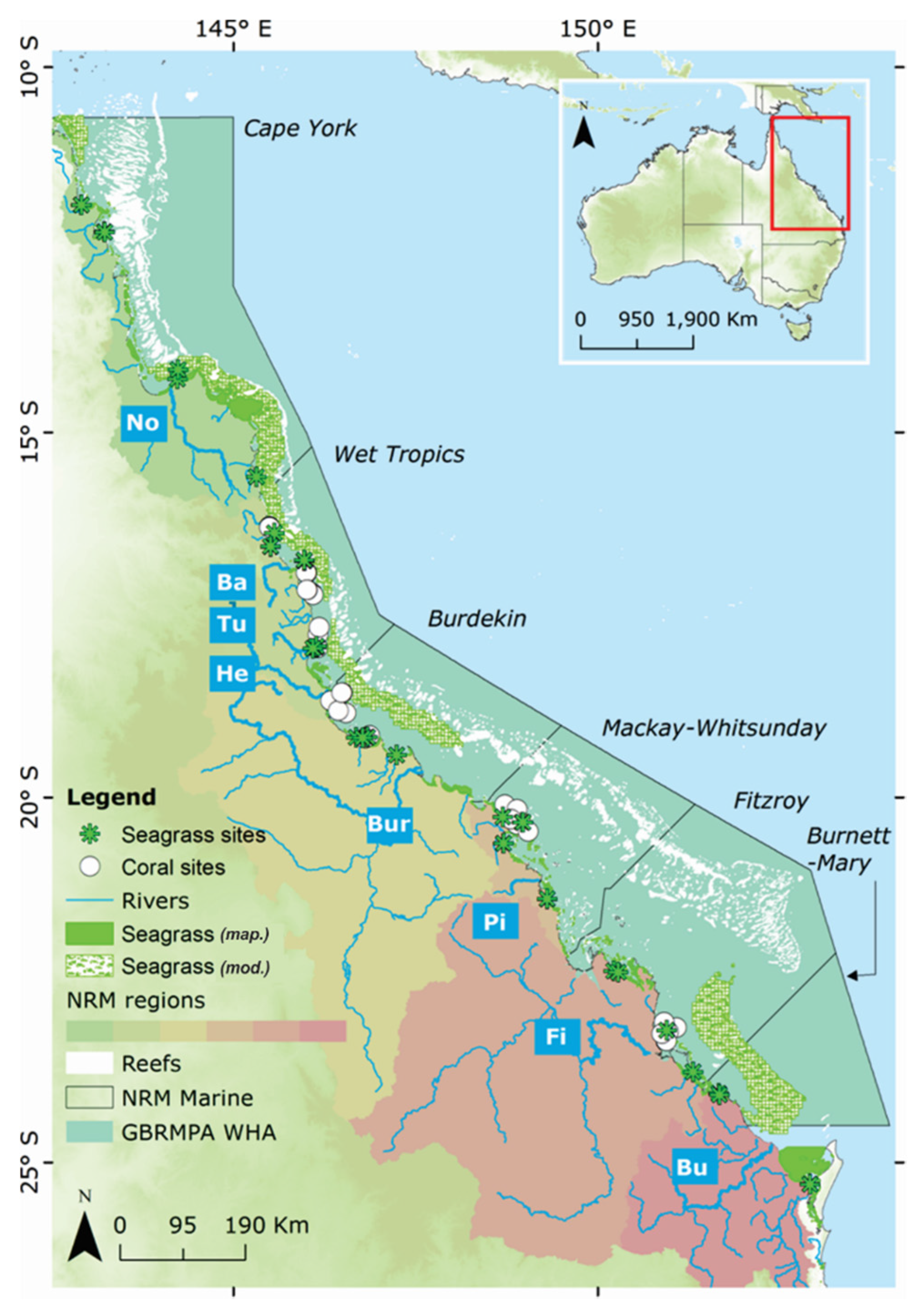
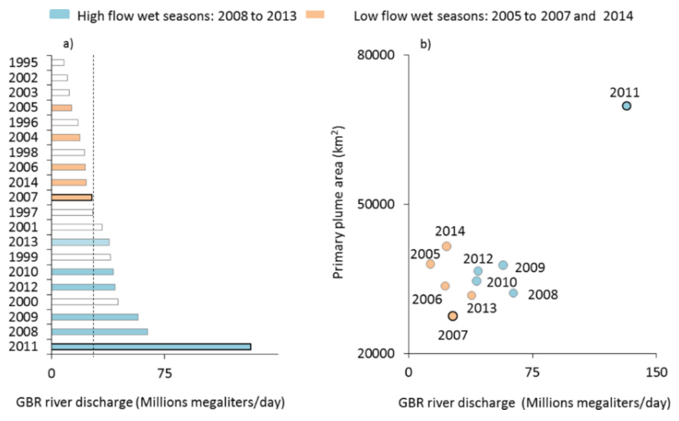
3.1. Mapping of the GBR Plume Water Types over 10 Wet Seasons

River plumes were mapped in this work using MODIS true colour imagery and the method of Álvarez-Romero et al. ([12] and the supplementary material (Material and Method section)). In this method, daily MODIS data focused on the wet season are classified into six colour classes corresponding to a gradient of six distinct plume water types. The six plume water types are hereafter referred to as plume colour classes 1 (CC1) to 6 (CC6). CC1–CC4 correspond to the Primary plume water type, CC5 to the Secondary plume water type and CC6 to the Tertiary plume water type of Petus et al. [16]. The method of Álvarez-Romero et al. [12] was used to classify 10 years of GBR MODIS images and to produce daily plume water type maps for the wet season 2005 (i.e., December, 2004–April, 2005) to the wet season 2014 (i.e., December, 2013–April, 2014). Coral reefs and land areas were masked out and weekly water type composite maps (22 composites per wet season) were created to minimize the amount of area without data per image, due to masking of dense cloud cover, common during the wet season [68] and intense sun glint [12].
Weekly composites were thus overlaid (i.e., presence/absence of each plume water type) and normalised (i.e., number of weeks divided by 22 wet season weeks) to compute seasonal normalised maps of frequency of occurrence for each plume water type (hereafter plume or water type frequency maps). Frequency values were extracted along a notional transect from the mouth of the Herbert River to illustrate that the extent and frequency of occurrence of the river plumes and water types was variable with distance from the coast and across wet seasons. Multi-annual composite maps were finally created by overlaying the seasonal composites in ArcGIS®10 and calculating the average frequency values of each cell/dry season. The Cape York region was removed from this analysis as it is a shallow environment where the remote sensing methods have not been fully validated [12].

3.2. Environmental Data: The Marine Monitoring Program (MMP)

The MMP undertaken in the GBR lagoon assesses the effectiveness of the Australian and Queensland Governments’ Reef Water Quality Protection Plan and the Australian Government’s Reef Rescue initiative. The MMP was established in 2005 to help assess the long-term status and health of GBR ecosystems, focusing on seagrass meadows and coral reefs. The current program includes the monitoring of ambient [69] and wet season [70] water quality and of seagrass [71] and coral reef [72] conditions.

3.2.1. Wet Season Monitoring of Water Quality

Water quality monitoring during the wet season characterises the acute and chronic influence of terrestrial runoff on water quality conditions that can, in turn, be used to assess effects on coral and seagrass health [15]. The design of the wet season monitoring program is detailed in, e.g., Devlin et al. [14,70] with documented QA/QC procedures [73]. Surface water samples are collected inside the visible extent of river plumes, in a series of transects away from the river mouths. Flood plumes originating from the major rivers between 10 and 27 degrees S are targeted. Water quality parameters collected in river plumes include nutrients and organic carbon (particulates and dissolved), Chl-a, TSS, herbicides, CDOM and Secchi depth. Depth profiling by CTD-casts, including Kd(PAR), temperature, dissolved oxygen and salinity, accompany each surface sample.
In this study, the Wet Tropics herbicide data was used as the surrogate for the GBR, as this was the most data-rich site throughout the sampled wet seasons. Herbicide measurements in this region were collected sporadically during the wet seasons 2010–2011 to 2012–2013 and more extensively during the wet season 2013–2014, but numbers of samples were limited, with a total of 86 key herbicides measurements collected. The key PSII herbicides measured in the Wet Tropics include Ametryn, Atrazine, desethyl-atrazine (DE Atrazine), desisopropyl-atrazine (DI Atrazine), Diuron, Fluometuron, Hexazinone, Prometryn, Simazine and Tebuthiuron residues (in ng·L−1). The key concentrations of these herbicides were normalised to an herbicide-equivalent concentration (PSII, μg·L−1), which is based on the relative toxicity of Diuron [74]. Each herbicide is attributed a toxicity factor relative to the Diuron toxicity (TF), where a TF equal to 1 indicates the same toxicity as Diuron at the same concentration. PSII concentration of any given grab sample was calculated as indicated in Equation (1), assuming these herbicides act additively [75,76,77].
P S I I =   i = 1 n ( H i × T F i )
where Hi stands for each sampled herbicide and TFi is the corresponding toxicity factor in relation to Diuron. TfAmetryn = 1.31, TfAtrazine = 0.16, TfDE_Atrazine = 0.11, TfDI_Atrazine = 0.003, TfDiuron = 1.00, TfFluometuron = 0.04, TfHexazinone = 0.38, TfPrometryn = 1.05, TfSimazine = 0.07, TfTebuthiuron = 0.08.

3.2.2. Seagrass Monitoring Programs

Seagrass monitoring undertaken under the MMP and Seagrass-Watch occurred from 2005 to 2014 at 23 locations inside the marine park boundary (Figure 1) and has been thoroughly described [45,71]. Meadows chosen for monitoring were lower littoral (rarely exposed to air) and subtidal (~2 m depth). Field survey methodology followed Seagrass-Watch standard protocols [78]. Sites were defined as a 50 m × 50 m or 50 m × 6 m area, for lower littoral and subtidal, respectively, within a relatively homogenous section of a representative seagrass community/meadow. Sites were monitored for seagrass abundance (% cover, hereafter: cover) and species composition. As the major period of runoff from catchments and agricultural lands is the wet season, monitoring was focused on the late wet season (March–April) and on the late dry season (October–November) during peak growth and expansion. Data were collected 3–4 times per site per year, and as flood-related losses of seagrass can occur during the 6 months following the flood [79], the late dry season cover data were selected in this study to capture the status of seagrass in relation to the previous wet season.

3.2.3. Coral Monitoring Programs

The cover of macroalgae is one of the bio-indicators used in the MMP to assess the current condition of the coral reef community [72]. The reefs monitored are typically fringing reefs of high islands located between 2 and 25 km from the mainland coast and so span the gradient of river plume exposure and turbidity associated with wind driven resuspension of shallow coastal waters (Figure 1). The proportion of total cover of benthic algae consisting of large fleshy species was derived from photo point intercept transects in which the percent cover of the substrate cover was estimated by identifying organisms beneath five points on each of 320 digital images (adapted from [80]) distributed over 10 × 20 m transects at 2 m depth below the lowest astronomic tide. Sites have been monitored annually or biannually in winter (May through August) since 2005. Recruitment, growth and biomass of macroalgae are controlled in part by nutrient availability [81]. In addition, a high abundance of macroalgae suppresses coral resilience (e.g., [82,83,84]) by increased competition for space or by changing the microenvironment into which corals settle and grow (e.g., [57,85]). A high macroalgal cover is widely accepted as an indicator of reef degradation and the macroalgae data were accordingly used here as an indicator of the likelihood of increased coral-algal space competition [72]. We considered the proportion of the total cover of algae on a reef that is comprised of macroalgae (hereafter referred to as proportional macroalgae cover or MAp in %), as opposed to the cover of macroalgae per se, as this allows the standardisation of macroalgae cover for space occupied by corals, loose sediments and other reef biota.

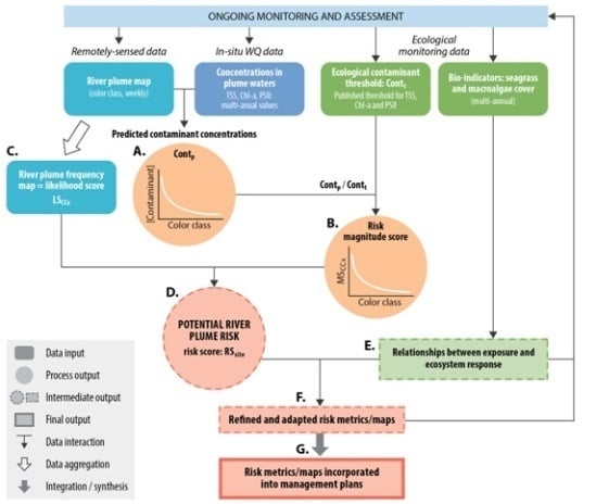
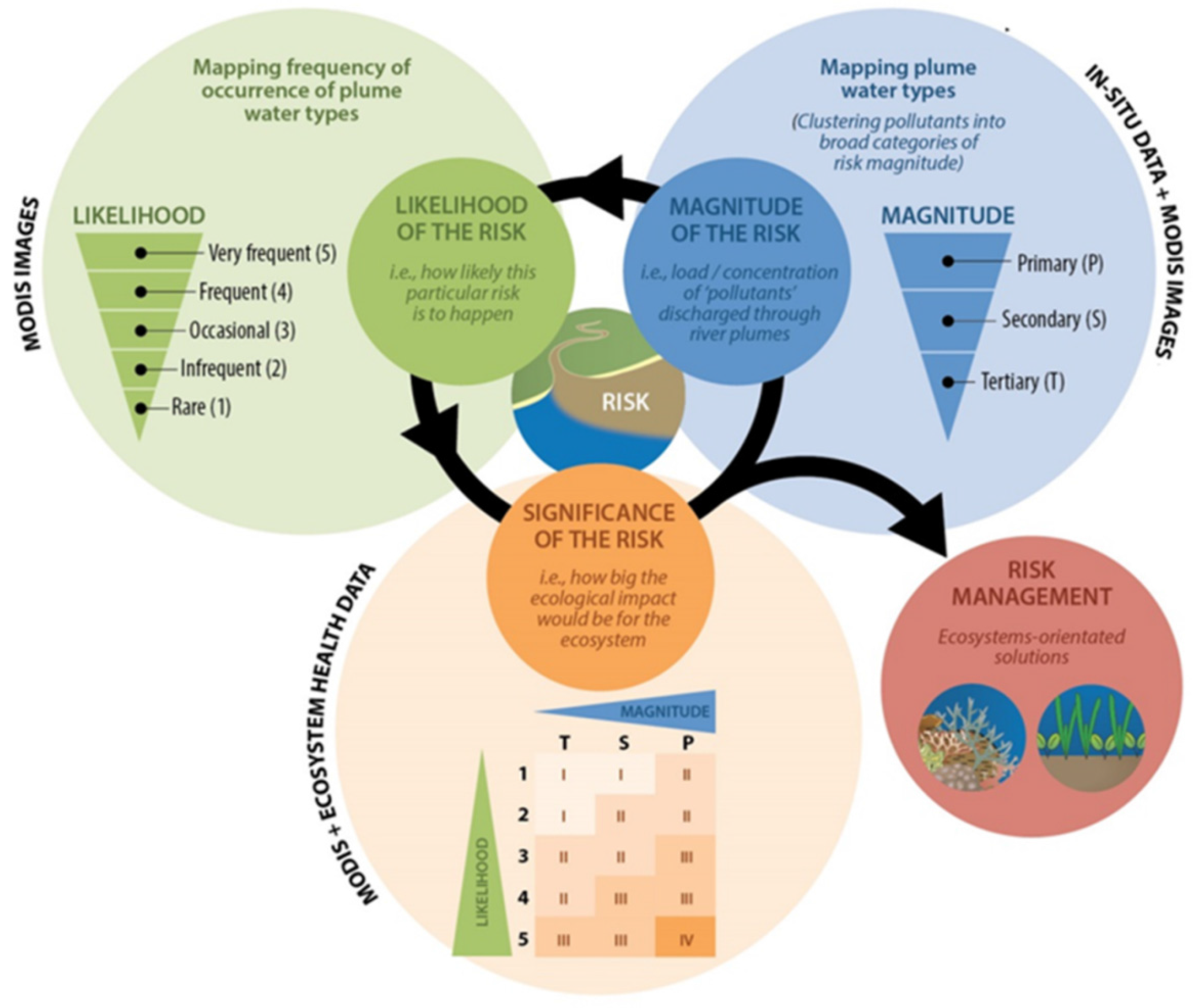
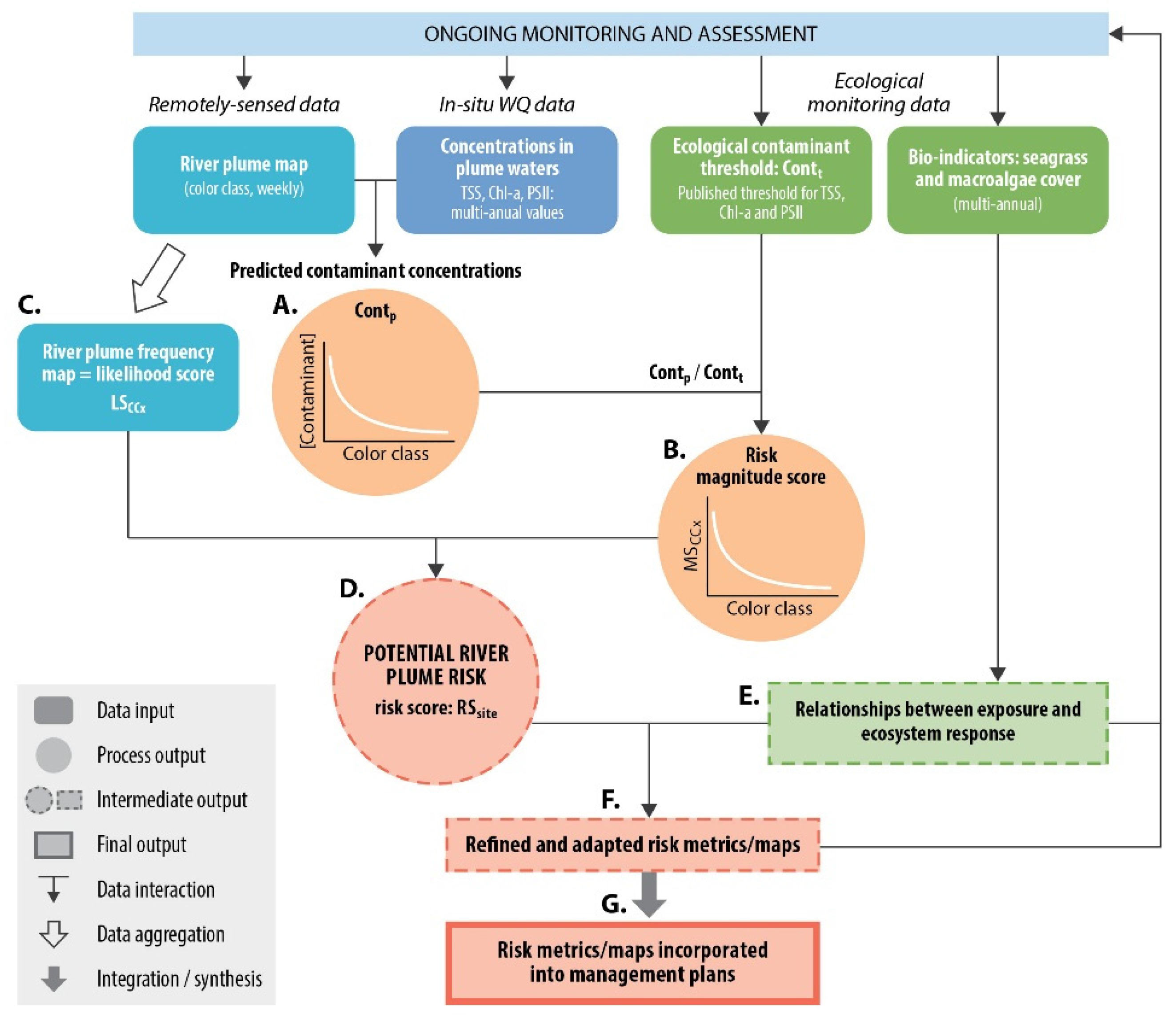
3.3. Testing of the Satellite Risk Framework

3.3.1. Magnitude Score

Average concentrations of TSS, PSII, DIN, DIP, Kd(PAR), Chl-a and CDOM measured in situ in each plume water type were calculated for every wet season (from 2005 to 2014), by comparing the weekly plume water type composite maps and in situ water quality measurements, collected as part of the Wet Season Program of the MMP (Figure 3A). In situ water quality values are assigned to weekly water masses CC1–CC6 based on their location, and data extraction were performed using the bilinear method implemented in the raster package of R 3.1 [86]. The mean value (× ± standard error) of TSS, PSII, DIN, Dissolved Inorganic Phosphorus (DIP), Kd(PAR), Chl-a, CDOM and PSII, as well as the mean salinity, was then calculated for each water type over the 2005–2014 sampling period. It has been shown that the herbicide residues in the GBR flood plumes are predominantly in the dissolved phase rather than bound to particulate materials [59], and change in herbicide concentrations across plume waters is believed to be principally controlled by a conservative mixing behaviour with the seawater rather than by a chemical or biological breakdown [60]. The number of PSII data available in each plume water type was limited and showed a non-conservative behaviour. A linear model was, thus, applied to the in situ data to estimate the multi-annual mean PSII concentrations per plume water type.
Ratios between predicted TSS, PSII and Chl-a concentrations in river plumes and the ecological thresholds were calculated and summed for each plume water type (Equation (2): RCCx). The ecological thresholds used were those published in Brodie et al. [26] (Section 2.3. and the supplementary material (Table S2)), i.e., TSS = 7 mg·L−1, Chl-a = 0.45 µg·L−1 and PSII = 0.1 µg·L−1. A cumulative risk magnitude score was then calculated for each plume water type (Figure 3B, hereafter Magnitude Score or MSCCx) by normalising across plume water type (Equations (2) and (3)). Concentration addition has been suggested as the “general solution” to the problem of calculating an expected quantitative effect for any combination of agents, and when their mechanisms of action are unknown [20,87,88,89].
R C C x =   T S S p C C x T S S t C C x + C h l a p C C x C h l a t C C x + P S I I p C C x P S I I t C C x
where p stands for the predicted concentration of each contaminant, t for the corresponding ecological threshold and CCx for an individual colour class (CC1 to CC6).
M S C C x =   R C C x   min ( R C C x ) max ( R C C x )   min ( R C C x ) × 10
where min(RCCx) stand for the minimum “RCCx across plume water type and “max(RCCx)-min(RCCx)” for the range of RCCx across plume water types.

3.3.2. Likelihood Score

The likelihood of exposure (defined here as the frequency of exposure) to each colour class at the seagrass and coral sites locations was extracted from the multi-annual water type frequency maps using ArcMap Spatial Analyst (ESRI, 2010). A 3 × 3 km buffer was created around each monitoring site and the multi-annual (2005–2014) frequency value of each pixel was extracted from the buffered area. Each seagrass and coral monitoring site was then assigned a multi-annual Likelihood Score (LSCCx) based on the averaged values extracted (Figure 3C).

3.3.3. Risk Score: Magnitude × Likelihood

The probability of exceeding ecological threshold concentrations from exposure to river plumes, i.e., the river plume risk to seagrass and coral reef ecosystems (RSsite), was estimated by multiplying each respective MSCCx by its LSCCx (magnitude × likelihood) and summing (Equation (4): RS’site), then normalising over all monitored sites (Equation (5)) (Figure 3D).
R S s i t e =   i = 1 n ( L S CCi   × M S C C i )
where LS stand for the Likelihood Score, MS for the Magnitude Score and CCi: the colour classes, (n = 6).
R S s i t e =   R S s i t e   min ( R S s i t e ) max ( R S s i t e )   min ( R S s i t e )
where min(RS’site) stand for the minimum RS’site across all monitored sites and max(RS’site)min(RSsite) for the range of RS’site across all monitored sites.

3.3.4. Relationships between Risk and Ecosystem Response

The seagrass and MAp data were used as bio-indicators of ecosystem response to test the initial validity of the risk maps. The long-term (2005–2014) response of seagrass and coral to river plume exposure was evaluated by calculating (i) the changes in seagrass cover and MAp across years 2005–2014 (Equation (6)) and (ii) the mean multi-annual seagrass cover and MAp (Equation (7)). Because the bio-indicator monitoring data were not always continuous at each seagrass and coral site (i.e., missing years), we interpolated between the years to get continuous times series. When no data was available for 2005 or 2014, the earliest and most recent ecosystem data available were considered (see the supplementary material (Tables S3 and S4)).
Δ B i o I n d i c a t o r = B i o I n d i c a t o r 2014   B i o I n d i c a t o r 2005
M B i o I n d i c a t o r =   1 n   i = 1 n B i o I n d i c a t o r i
With bio-indicators: seagrass meadow cover or MAp and i: the monitoring year (2005–2014, n = 10)
Finally, the hypothesis that long-term (2005–2014) responses of coral reefs and seagrass meadows will be influenced by contaminant concentrations and frequency of exposure to the contaminant concentrations was investigated by correlating biological bio-indicator responses (Equations (6) and (7)) to their risk score at the site (Equation (5): RSsite) and NRM regional scales (by averaging all sites within a same NRM region: RSNRM) (Figure 3E).

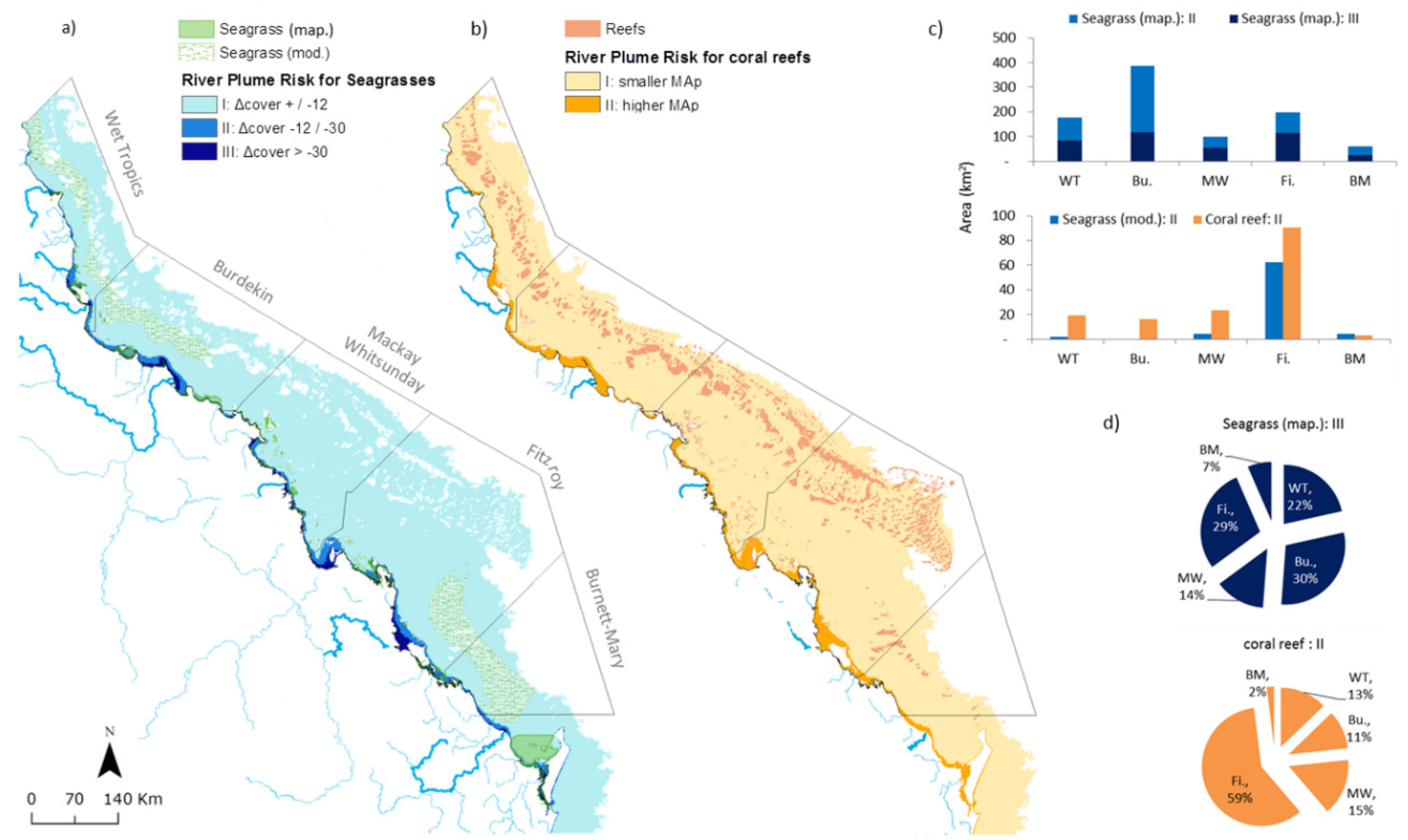
3.4. Spatial Distribution of Risk of Seagrasses and Coral Reefs to River Plume

The above correlations were used to derive multiannual risk score thresholds and relative risk categories for loss of seagrass cover and higher MAp, as well as to generate river plume risk maps specifically for seagrass meadows and coral reefs of the GBR (Figure 3F). The exposure of GBR marine ecosystems was expressed simply as the area (km2) and percentage (%) of coral reefs and seagrass meadows within each NRM region that were exposed to different categories of river plume risk. Figure 1 presents the marine boundaries used for the GBR Marine Park, each NRM region, and the seagrass (mapped and modelled) and coral reefs ecosystems. Seagrass meadows of Hervey Bay (which is outside of the GBR southern boundary, Figure 1) were not included in the risk analysis.

4. Results

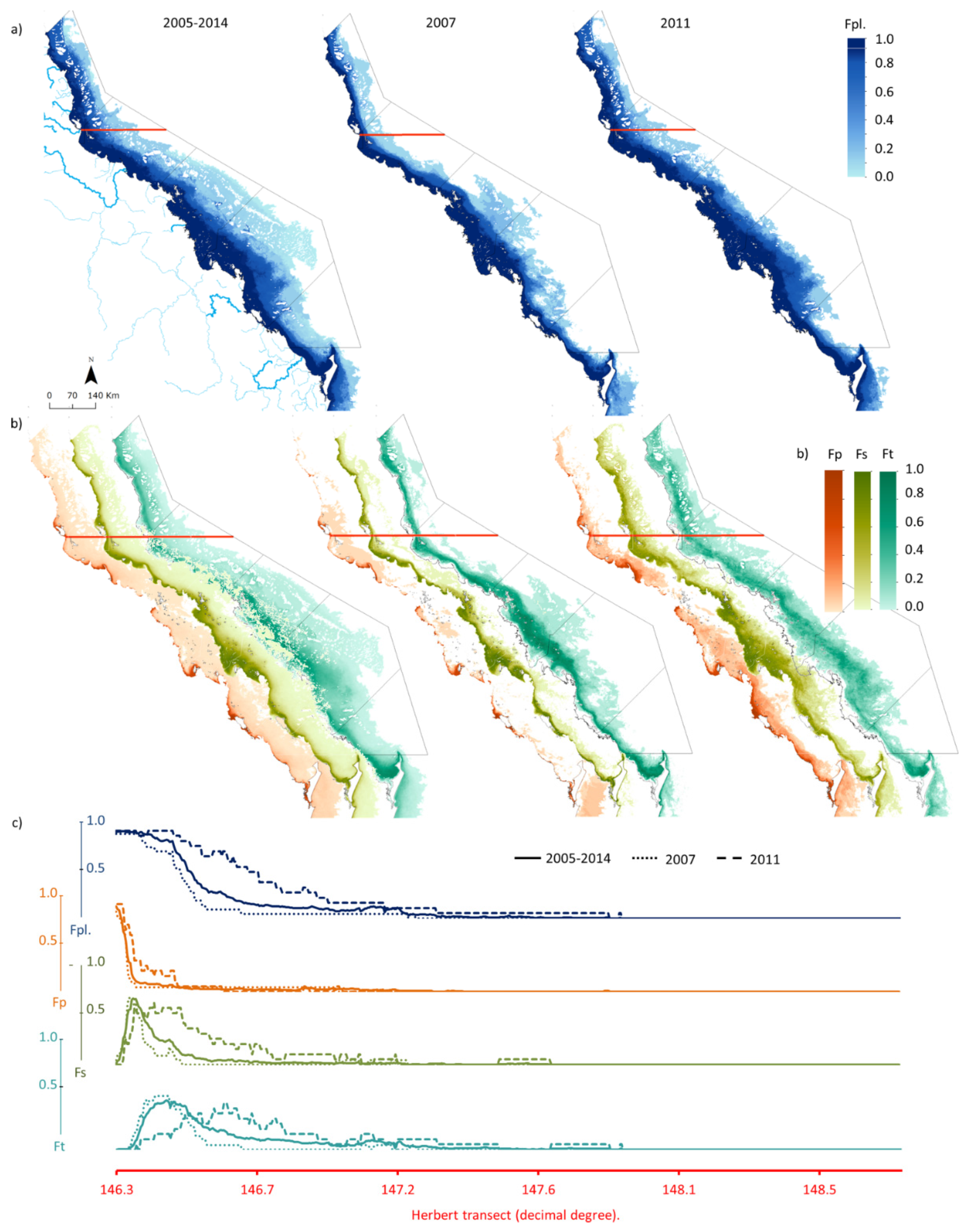
4.1. Mapping the Water Types in Flood Plumes

This study covered ten wet seasons (2005–2014) in which there were four wet seasons with low (total river discharge below the 20-year median) river flows (2005–2007 and 2014) and six with high (total river discharge over the 20-year median) river flows (2008–2013) (Figure 4a). The 2011 wet season was an extreme wet season, with a river discharge about 5 times the 20-year median value.
The extent and frequency of occurrence of the river plumes and water types was variable across regions, cross-shelf and wet seasons, reflecting the constituent concentrations and intensity of the river discharge (Figure 4b and Figure 5). Despite this variability, the primary (turbid plume) waters were generally limited to a small near-shore zone (<10 km across the shelf) and, on average, 38,281 km2 (11%) of the GBR lagoon was exposed to primary plume waters (Figure 4b). This area increased during the wettest wet seasons and decreased during the driest wet seasons (Figure 4b and Figure 5). The maximum area of primary water was recorded in 2011 (69,745 km2, or 20% of the GBR). The extent of the secondary (CC5) and tertiary (CC6) flood plume frequency is rarely attributed to an individual river and is usually merged into one heterogeneous plume [90]. On average, the secondary and tertiary plume waters covered 25,000 km2 of the GBR lagoon and 43,000 km2, respectively.

4.2. Contaminant Concentrations across Plume Water Types

The mean salinity linearly decreased from the CC6 to the CC1 water type (Figure 6a and the supplementary material (Table S5)) and the variation of water concentrations across the six water types followed the expected gradients over multi-annual time-scales [13,15,90]. Most of the water quality parameters, including Kd(PAR), TSS, DIN and DIP, decreased across the six plume water types (Figure 6a and the supplementary material (Table S5)). Highest TSS concentrations were recorded in the coastal colour class (34.0 ± 60.8 mg·L−1 in CC1) and dropped rapidly as the heavier particles settled, with only the finer colloidal sediment moving further offshore in the plume waters [91]. The highest Chl-a concentrations were measured in the CC1–CC3 with maximum values recorded in CC1 (2.4 ± 3.2 μg·L−1) and a slight decrease in concentration from CC2–CC3 (2.1–2.0 μg·L−1). Chl-a concentrations varied between 1.4 ± 1.3 and 0.9 ± 0.7 μg·L−1 in CC4 and CC5 and deceased to 0.4 ± 0.6 μg·L−1 in the offshore plume waters. The number of PSII data available in each plume water type was limited (less than 10 data in CC1, CC2, CC3 and CC6 and 29 data in the CC4 and CC5, respectively) and showed a non-conservative behaviour (Figure 6b). Based on the linear model (Figure 6b), mean multi-annual PSII concentrations were, respectively, 0.04 µg·L−1, 0.02 µg·L−1 and 0.01 µg·L−1 in CC1, CC4 and CC6.
Mean multi-annual concentrations of TSS and Chl-a were over the ecological thresholds in all plume water types, except in CC6 where MSCC6 was scored as zero (Table 2). However, estimated mean PSII concentrations were all under PSII = 0.1. Ratios of contaminant concentrations against ecological thresholds increased across the plume water gradient (toward the inshore CC1 plume water type). Mean concentrations of TSS and Chl-a were more than 1.5 and 4.0 times higher than threshold concentrations in the CC3, respectively, and about 5 times higher in the CC1. As a result, the normalised Magnitude Score increased from the offshore (Table 2: MSCC6 = 0) to the inshore (MSCC1 = 10) plume waters, with a sharp increase of the combined Magnitude Score in the CC1 vs. CC2 or CC3 (MSCC2/CC3 = 5).

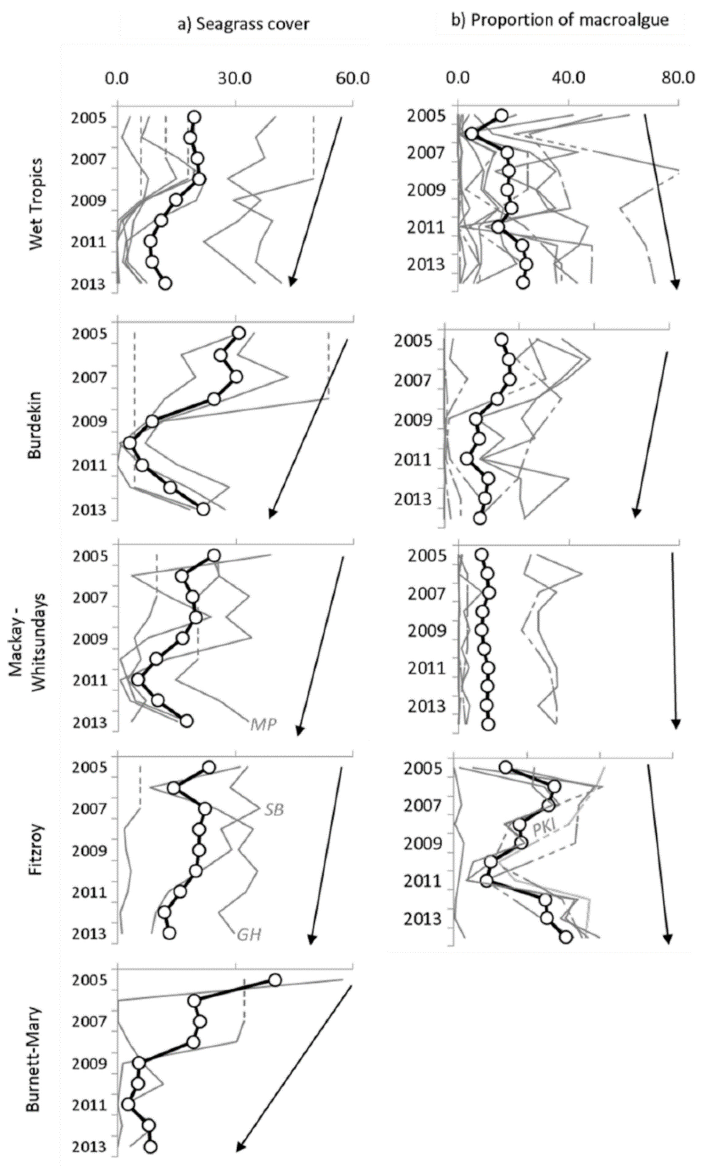
4.3. Environmental Data: Seagrass Meadows and Proportional Macroalgae Cover in the Algal Communities

Seagrass meadow cover declined from 2005 to 2014 (though with some recovery after 2011) in all NRM regions of the GBR (Figure 7a: black arrows and Table 3). The largest changes in seagrass cover occurred in the Burnett Mary NRM region with a loss of 43.2% of cover (Table 3: ΔBM), and a mean multi-annual cover of 12.4% (Table 3: MBM). The smallest changes occurred in the Mackay Whitsunday (ΔMW= −7.1%) and the Wet Tropics (ΔMW = −7.5%). Mean multi-annual cover for both of these regions was about 15.3% and 15.0%, respectively. At the site level, maximum changes were measured at the Urangan sites (Table 3: ΔUG = −54.1%) and minimum changes at the outer Gladstone Harbour sites (Table 3: ΔGH = −1.40%).
The proportional macroalgae cover (MAp) was highly variable through time and between regions (Figure 6b: black arrows and Table 4) compared to that of seagrass meadows. The Fitzroy NRM region showed a clear increasing trend of MAp across the years 2005–2014 (ΔFi = +32.7%) and the highest mean multi-annual MAp of the GBR regions (MFi = 41.0%). Increasing trends were also observed at the Wet Tropic reefs (ΔWT = +7.8%), while a decrease in MAp was measured in the Burdekin region (ΔBu = −11.1%). No trend could be observed at the Mackay Whitsunday reefs (ΔMW = +2.5%), with macroalgae only common at the Pine Island and Seaforth Island sites where it has maintained a reasonably consistent representation in the algal communities (ΔPI = 8.9%, ΔSI = 7.0%, MPI = 31.0% and MSI = 31.8%).

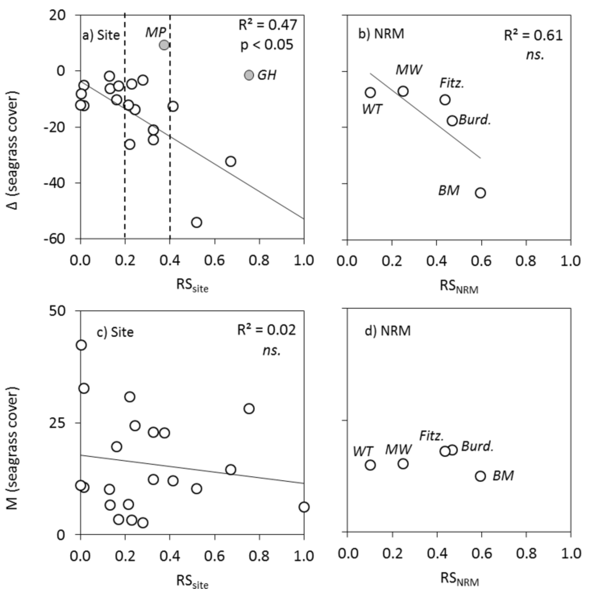
4.4. Relationships between Plume Exposure and Seagrass Response

Multi-annual changes in seagrass cover (Δsite) across sites were negatively correlated to their risk scores (RSsite; Table 3); however, Gladstone Harbour and Midge Point appeared to be outliers of the observed relationship (Figure 8a: R2 = 0.47, p < 0.05). At the regional (NRM) scale, no significant relationship was found between ΔNRM and RSNRM (Table 3 and Figure 8b, R2 = 0.61, ns.). However, the relatively lower loss of cover in the Wet Tropics and Mackay Whitsunday NRM regions (Table 3: ΔWT = −7.5% and ΔMW = −7.1%) was associated with the lowest regional risk scores (Table 3: RSWT = 0.1 and RSMW = 0.2). Inversely, the higher loss in cover observed in the Burnett-Mary region (Table 3: ΔBM = −43.2%) was associated with the highest risk score (RSBM = 0.6). No significant relationships were found between the mean multi-annual seagrass cover values and the risk scores at the site and regional scales (Figure 8c,d).
The correlation between the multi-annual changes in seagrass cover and risk scores at the site level (Figure 8a) were used to derive multiannual risk score thresholds and relative risk categories for loss of seagrass cover (Table 5: I, II and III). The risk score thresholds were manually optimised to have fewest sites with an underestimated loss of seagrass cover (a conservative approach, whereby there is a greater chance of identifying high risk than not identifying it). The following risk score thresholds were selected: a RS ≤ 0.2 was associated with a gain or the lowest loss in seagrass cover (Δcover: gain/−12%, hereafter risk category I), 0.2 < RS ≤ 0.4 was associated with moderate loss (Δcover: −12/−30%, hereafter risk category II), and a RS > 0.4 was associated with the greatest loss in cover (Δcover>−30%, hereafter risk category III). Using this conservative approach and the selected risk score thresholds, 14 out of the 20 (70%) monitored seagrass sites had their multi-annual loss in cover well estimated and only one site had an underestimated loss in cover (Table 5).

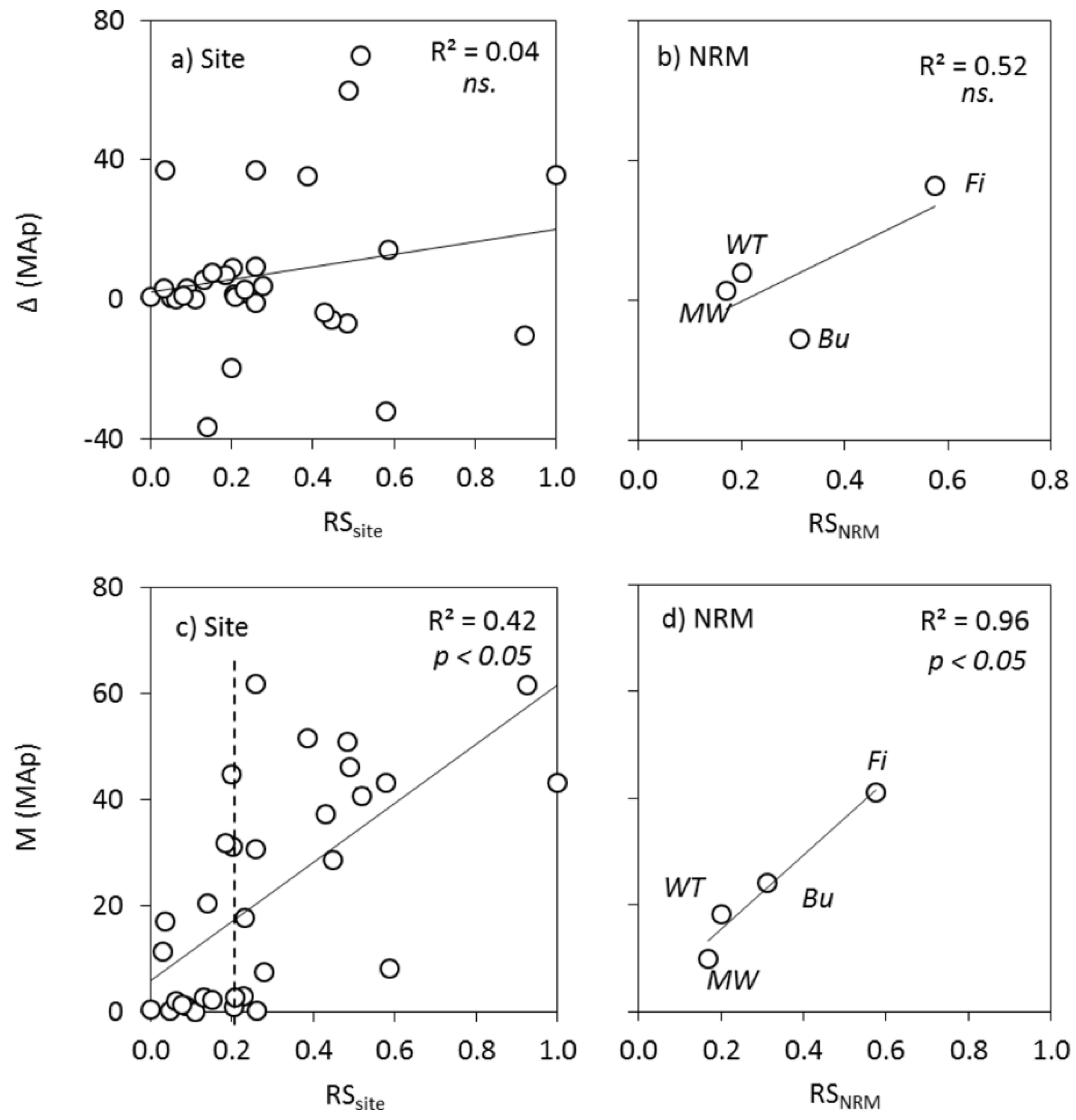
4.5. Relationships between Plume Exposure and MAp Response

Multi-annual trends in MAp were highly variable both through time and between regions (Figure 7b) and the interactions between risk scores and multi-annual changes in MAp were complex (Table 4 and Figure 9a). At the site scale, a slight increase of the Δsite with increased RSsite values was observable, but was not significant (Figure 9a, R2 = 0.04, ns.). At the regional scale, trends were clearer though still not significant (Figure 9b, R2 = 0.52, ns.). Relatively stable multi-annual trends in the MAp cover of the Mackay Whitsunday and Wet Tropics or loss of MAp cover in the Burdekin NRM regions (Figure 7b) were associated with similar low regional risk scores (Table 4 and Figure 9b: RSNRM = 0.17–0.31). Inversely, the increasing trend in MAp cover observed in the Fitzroy NRM region was associated with the highest risk scores (RSFitz. = 0.58).
Stronger relationships were observed by considering the mean multi-annual MAp values (Figure 9c,d) rather than the MAp changes across years 2005–2014 (Figure 9a,b). Significant relationships were observed, and suggested an increase of the mean multi-annual MAp with increased risk magnitude scores, at both the site (Figure 9c, R2 = 0.42, p < 0.05) and regional scales (Figure 9d, R2 = 0.96, p < 0.05). The correlation between the multi-annual MAp and risk scores at the site level (Figure 9c) were used to derive a multiannual risk score threshold and two relative risk categories for MAp. Seventy percent (14 out of 20) of the monitored coral sites with RS > 0.2 had a mean multiannual MAp > 10%, while only 33% (4 out of 12) monitored coral sites with RS ≤ 0.2 had a mean multiannual MAp > 10%. A threshold of about 0.2 was thus selected under/above which a smaller/higher (risk categories I/II) MAp at the reef sites can be expected.

4.6. River Plume Risk Map

River plume risk maps were generated from the multi-annual water type frequency maps and the above risk score thresholds (Figure 10). They show the spatial distribution of risk of seagrasses (Figure 10a) and coral reefs (Figure 10b) to river plumes in the GBR. The area of higher risk for the seagrass meadows (risk categories II and III) and the coral reefs (risk category II) was limited to a narrow coastal band (5 to 20 km), representing 3%–4% of the GBR (minus the Cape York region).
Considering the area of seagrass meadows (Figure 10a: map. and mod.) exposed to river plume risk categories within the regions included in this study (excludes Cape York), 38% (527 km2) and 29% (395 km2) of the coastal (map.) seagrass meadows were within the risk categories II and III, respectively (Figure 10c). One hundred percent of the deepwater (mod.) seagrass meadows were within the risk category I. Of the coastal seagrass exposed to the risk category III, 30% (117 km2) and 29% (113 km2) were in the Burdekin and Fitzroy regions, respectively (Figure 10d). Considering the area of coral reefs exposed to river plume risk categories (Figure 10b: excludes Cape York), the majority (89% or 12,212 km2) were within risk category (I) and only 1% (153 km2) was within the risk category II (Figure 10c). Ten percent of the reef area was beyond risk of plume exposure. Of the reefs exposed to the risk category II, 59% (90 km2) were in the Fitzroy region with similar proportions (11%–15%) in each of the Burdekin, Wet Tropics and Mackay Whitsunday regions (Figure 10d).

5. Discussion

This study contributes to the development, test and validation of innovative remote sensing monitoring tools currently undertaken in the GBR in order to understand the relationships between pressures from human activities, including influences on coastal water quality, and their effects on marine ecosystems [15]. It contributes to adaptive management approaches developed to set relevant frameworks and thresholds for adverse biological responses and to map spatial risk in the GBR. The ecological and risk score thresholds used in this study will be refined and validated through ongoing monitoring and assessment (Figure 3F). However, the risk framework proposed here is designed to help GBR scientists and managers that aim to mitigate the risk of degraded water quality to local ecosystems and provides an important data visualization tool for communicating environmental risks to stakeholders such as the general public and policy makers [38]. It is readily applicable to other regions of the world, given that the ecological and risk thresholds are regionally adjusted following the processes proposed here.
This study confirms that levels of TSS and Chl-a in GBR river plume waters exceed published ecological thresholds, except in the most offshore CC6 plume water type, and generally decrease from the inshore to offshore plume water types (Figure 6 and Table 2). Estimated mean herbicide concentrations in river plume waters were below the biological response threshold in all plume water types and therefore risk from exposure to PSII herbicides in river plume waters was scored as zero in the risk scores. It should be noted, however, that given the persistence of herbicides in coastal waters [88], sublethal chronic impacts can occur even at low concentrations [62]. The majority of herbicides of environmental concern in the GBR are soluble in water rather than bound to particles [59], and therefore this study assumed conservative mixing behaviour with the seawater. However, relatively high concentrations of the herbicide Diuron have been found in sediments [92] with potential risk to seagrass health [93]. As a result, the risk assessment presented in this study might underestimate risk from herbicide exposure.
The highest in situ Chl-a concentrations were measured in coastal plume waters, with maximum values recorded in CC1 and similar values in CC2 and CC3 (Table 2: 1.95–2.41 μg·L−1). High TSS in the CC1 plume water type is expected to inhibit phytoplankton productivity and Chl-a concentrations [70,90]; therefore, freshwater phytoplankton or detritus transported by GBR Rivers, could explain the relatively high Chl-a concentrations. With the exception of the CC2 and CC3 plume water types, which scored the same (RSCC2 and RSCC3 = 5) as a result of very similar Chl-a and TSS concentrations, risk scores generally decreased from CC1–CC6, supporting the assumption that the magnitude of risk decrease across the river plume gradient [16].
Comparing Risk Framework outputs with seagrass and coral ecosystem health is important to validate theoretical risk thresholds. The Satellite Risk Framework and risk scores presented in this study were successful in demonstrating where plume conditions are, on average, associated with adverse ecological responses over multi-annual time-scales. The correlation between the multi-annual changes in seagrass cover and risk scores at the site level (Figure 8a) were used to derive multiannual risk thresholds associated with loss of seagrass cover (Table 5). From these scores, a plume exposure risk map for GBR seagrass meadows has been developed (Figure 10a). Furthermore, this initial analysis provided evidence of a link between river plume exposure and proportional macroalgae cover (Figure 9c). A multi-annual risk score threshold of 0.2 was proposed, above which a high proportion of macroalgue in algal communities at these reef sites can be expected (Figure 10b). This result helps to further resolve the area of high water column concentrations of Chl-a, and total suspended solids previously identified as corresponding to higher abundance of macroalgae [48] and to maps GBR areas within which macroalgae could be expected to be a major space competitor of hard corals.
The area of higher risk for the seagrass meadows and the coral reefs was limited to a narrow coastal band and the area of coral reefs and seagrass beds in each river plume risk category varied between NRM regions and ecosystems (Figure 10). Seagrass meadows have relatively high light requirements [47] and are often restricted to the shallow coastal waters. This places them at higher risk of exposure to river plume waters, and 29% of the GBR coastal seagrass meadows were within the highest relative risk area for seagrass meadows. Inversely, only few coral reefs were located within the highest relative risk area for coral reefs, suggesting that issues related to enhanced completion between macroalgae and coral communities on the GBR are limited to a relatively small proportion of coral reefs (about 1%). The river plume risk was greatest for coral reefs in the Fitzroy and Mackay Whitsunday regions, and for coastal seagrass meadows in the Burdekin and Fitzroy regions. These results are similar to the results from the GBR Risk Framework that assessed the risk of pollutants to GBR ecosystems using comprehensive water quality and environmental datasets [26]. This underlines the potential of using simple supervised classification of true colour satellite imagery in combination with in situ water quality data to estimate the likely adverse effect of combined contaminants in river plume waters on ecosystems.
This study focused on multi-annual analyses to test the initial validity of the maps produced from the Satellite Risk Framework. However, exceptions to the general trends highlight that underlying ecological processes governing short-term and small-scale fluctuations in seagrass and proportional macroalgae cover could not be resolved. For example, seagrass meadow responses at outer Gladstone Harbour and Midge Point deviated from the general response to long-term exposure to river plume (Figure 8a), underlining the complexity of relationships existing between ecosystem response and water quality condition. The outer Gladstone Harbour site is at a location with relatively little catchment input [71] and is characterised by a good multi-annual state of seagrass cover, while onset of seagrass recovery has been observed at Midge Point since 2010 (Figure 7a, Fitzroy region: “GH” and Mackay Whitsunday region: “MP”). Specific resilience characteristics of seagrass species assemblage at each of the monitored sites, as well as other environmental conditions within seagrass meadows, also influence the response of individual sites within the regional groupings. Environmental conditions such as cyclonic activity [71], temperature and salinity [18], bathymetry and sediment type [94], tide currents and wave exposure (see references in [46]), or the zonal location of the meadows may have also contributed to the response of seagrass meadows. For example, very shallow intertidal meadows that receive light before, during, and immediately after low tide [95] exhibited the smallest loss in area compared to permanently submersed meadows [19]. Most of the sites considered in this study were occasionally exposed at low tide and this may also have affected how well seagrass responses corresponded to risk from plume water in this study. Furthermore, Wet Tropics sites had low overall risk scores, but a number of sites were under the direct pathway of TC Yasi, which caused physical removal of seagrass in that year (2011, see Figure 7a), and removed the source of propagules for recovery, thus maintaining low overall abundance in subsequent years [71].
The plume water types are characterised through the mapping of river plumes by MODIS true colour images recorded during the wet season [12], as it is typically during these periods of high flow that water quality is measured as a gradient from the inshore to the offshore boundaries of river plumes [13]. At the whole GBR scale, restricting the analysis to wet season months also minimises the occurrence of “false” river plume areas associated with wind-driven re-suspension of sediments during the strong trade winds typical of the dry season [12]. However, in shallow coastal areas of the GBR, muddy sediments can be re-suspended by wind, waves and tidal currents [96], increasing turbidity levels in coastal waters and resulting in misclassification of some pixels. This could explain the relatively high risk score calculated at the shallow Gladstone Harbor site (Figure 8a) for example, where very little cover loss was observed at this site, known to have relatively little catchment input [71]. The Gladstone Harbor seagrass meadows are also intertidal meadows, which are exposed to higher light levels than subtidal sites, which may have contributed to the smaller losses in cover observed at this site than other subtidal sites at similar plume exposure levels.
The lack of a consistent increase in macroalgae within algal communities over the period of increased risk of exposure to river plumes, along with observed high levels of variability at individual reefs over time (Figure 7b and Figure 9a), indicate the influence of processes not directly linked to the water quality parameters summarized by the risk score. A number of factors, including the suitability of the substrate and grazing pressure are understood to influence the abundance of macroalgae on coral reefs (e.g., [81,82]). Consideration of these factors was beyond the scope of this study, though they will likely have added to the variability in community responses observed. In addition, the macroalgae considered represent a grouping of a high number of species [72] with potentially differing responses to environmental conditions, which may have obscured mean effects. The multi-annual risk score threshold of 0.2 limited the river plume risk of coral reefs to a narrow band along the coast (Figure 10b) and many of the monitored reefs included in this study were situated beyond this threshold. This would likely cause a lack of short-term response to inter-annual variation in risk scores, as even though risk scores varied at many reefs, they never approached the risk score threshold indicated. Several of the more offshore reefs received little additional exposure over the period of this study; a consistently low cover of macroalgae implied these reefs are beyond the threshold that allows macroalgae to flourish. Conversely, high representation of macroalgae at many of the more inshore reefs prior to the onset of the wet period of 2008–2012 suggests that those algal communities were not environmentally limited (Figure 7b).
In addition, the relationship between increased risk score and a macroalgae response should not be expected to be uniformly linear due to the myriad of interactions between river plume exposure and other processes operating to control not just algae but all species within these complex ecosystems. As an example, turbidity and Chl-a concentration (as a proxy for nutrient availability) are aggregated into the risk score, however, these two factors can have competing influences on macroalgae. There is ample evidence that availability of nutrients is positively related to macroalgae abundance, but only where sufficient light is available [97], meaning that in the highly turbid conditions experienced in a plume, reduced light availability may outweigh any influence of enhanced nutrient supply. The observed reduction in macroalgae following large flood events on the reefs, with high magnitude exposure risk following large floods of the Fitzroy River, support this interpretation [72]. Despite this short term variability in macroalgae commuities as a direct response to flood exposure, the general increase in macroalgae cover on reefs in the Fitzroy region corresponded to a high risk score in this region (Figure 9b). Exposure to flood plumes in this region appears to have been not only a cause of coral mortality, but also a vector for the maintenance of water quality conditions suitable to the subsequent colonization and maintenance of high macroalgae cover.
Results obtained are encouraging, and the next steps should focus on progressing toward the production of annual river plume risk maps for GBR ecosystems. Such annual maps would inform a seasonal water quality context for GBR ecosystems and would provide the temporal scale necessary to resolve processes that govern short-term fluctuations in seagrass and proportional macroalgae cover. For example, they would help to determine the number of consecutive years a coral/seagrass ecosystem needs to receive a certain category of risk to see a shift in species response as a result of being exposed to reduced water quality in river plume waters. Such short term assessment has been initiated in the GBR, with preliminary results suggesting that exposure to plume waters from 10% to 60% of the wet season and during two consecutive wet seasons, could result in a significant loss of seagrass cover (>50%) [18]. Plume exposure thresholds varied in function of the cross-shelf location of the seagrass habitat and the ambient water quality conditions, but recovery processes after losses were not resolved [18]. Finally, the use of multidimensional statistics would help to progress understanding of the mechanisms of influence of the key water quality parameters associated with river plume waters, as well as additional external (e.g., environmental or competitive) and internal (e.g., physiology) pressures on seagrass and macroalgae responses.
In the present study, ecological thresholds above which impacts of plume exposure on ecosystems have been observed were defined following Brodie et al. [26]. However, only limited information is available to draw conclusions, for example, on the effects of exposure to sediments and nutrients (measured as Chl-a concentrations) on seagrass health. Experiments on the responses of GBR key species to interactive effects of these water quality parameters should be carried out to progress the development of final risk thresholds for GBR seagrass [18] and coral reefs. It is important to note that there are a multitude of pathways through which water quality may reduce the resilience of coral communities; among these are the increasing susceptibility to thermal stress and enhancing the survival of the crown-of-thorns starfish [98,99,100]. As the threshold for plume exposure risk will almost certainly differ, risk maps tailored to additional indicators of coral reef condition, or resilience, should be considered in later analyses, following the risk framework presented here. As risk metrics are adapted and improved with continual validation and reduced uncertainty, it will be possible to incorporate these products into applied management actions as useful tools to monitor and mitigate water quality impacts on ecosystem health (Figure 3G).

6. Conclusions

This study contributes to the development of remote sensing monitoring tools and to the adaptive management approaches developed to map spatial risk of ecosystem to river plume exposure in the GBR. The Satellite Risk Framework and newly-introduced risk score allowed the definition of a set of multi-annual risk thresholds associated with loss of seagrass cover and an intermediate river plume risk map specifically for seagrass meadows was generated. Considering a multiannual Risk Score threshold of 0.2, above which a high proportion of macroalgae within the algal communities at reef sites can be expected, allowed the identification of a relatively narrow coastal band within which macroalgae could be expected to be a major competitor of hard corals. This underlined the potential for using simple supervised classification of true colour satellite imagery in combination with in situ water quality data to map the likely adverse effect of combined contaminants in river plume waters on ecosystems. These risk maps will be validated by ongoing monitoring and assessment. They can be used in future to quantitatively assess ecosystems at greatest risk from plume water contaminants and, therefore, prioritise investment into water quality improvement.

Supplementary Materials

The following are available online at www.mdpi.com/ 2072-4292/8/3/210, Figure S1: from Devlin et al. [26], Modified from [24,25]): Summary of the process followed to build plume water maps with examples of inputs and outputs: (a) Plume mapping process: different shadings represent steps (light gray), analyses within steps (white), intermediate outputs (dark gray), and final outputs (black); (b) A: MODIS-Aqua true colour image used to create the spectral signature defining 6 color classes for GBR plumes (25 January 2011), B and C: daily 6-color class map (25 January 2011) and weekly composite (19 to 25 January 2011) of 6-class map. D: reclassified map into weekly P, S, T composite (19 to 25 January 2011); E: Frequency of occurrence of the secondary water type in 2011; Figure C to E are zoomed in the Tully-Burdekin area (see red box on panel B); Table S1: Operational bio-optical algorithms tested for the retrieval of WQ data gradients [1]; Table S2: Summary of water quality variables (WQv) and risk assessment classes defined in Brodie et al. risk assessment framework [10]. Magnitude and Likelihood categories (VR: Very Rare, R: Rare, O: Occasional, F: Frequent, VF: Very Frequent) and final risk categories (likelihood x magnitude): VL: Very Low, L: Low, M: Medium, H: High, VH: Very High are from published values or estimated by expert opinion. Likelihood categories for TSS and Chl-a are based on frequency of exceedance of the water quality threshold using remote sensing data and PSII categories are based on a recent assessment of to PSII (modified from [10,11]); Table S3: Proportion of macroalgue in the algal communities (MAp) measured through the MMP. Interpolated data are indicated in italic and with an asterisk; Table S4: Seagrass cover data measured through the MMP. Interpolated data are indicated in italic and with an asterisk; Table S5: Mean and standard deviation of water quality concentrations measured in the plume water types (CC1 to CC6).

Acknowledgments

We acknowledge the Australian Government funding under the Reef Rescue Marine Monitoring Program, the Australian Government's Reef Programme and specifically thank the Great Barrier Reef Marine Park Authority and Department of Environment for financial and technical support under this program. We acknowledge the Pesticide monitoring program under the MMP, particularly Christie Gallen and Chris Paxman. Authors also gratefully acknowledge support from the Centre for Tropical Water and Aquatic Ecosystem Research (TropWATER).

Author Contributions

Caroline Petus had the original idea for the study and, with Michelle Devlin, Angus Thompson and Len McKenzie carried out the conception and design of the study. Michelle Devlin, Angus Thompson, Len McKenzie, Eduardo Teixeira da Silva were responsible for the acquisition of data. Michelle Devlin, Angus Thompson, Len McKenzie, Eduardo Teixeira da Silva, Catherine Collier, Dieter Tracey and Katherine Martin helped with the analysis and interpretation of data. Caroline Petus drafted the manuscript, which was revised by all authors. All authors read and approved the final manuscript.

Conflicts of Interest

The authors declare no conflict of interest.

References

  1. Tilman, D.; Fargione, J.; Wolff, B.; D’Antonio, C.; Dobson, A.; Howarth, R.; Schindler, D.; Schlesinger, W.H.; Simberloff, D.; Swackhamer, D. Forecasting Agriculturally Driven Global Environmental Change. Science 2001, 292, 281–284. [Google Scholar] [CrossRef] [PubMed]
  2. Diaz, R.; Rosenberg, R. Spreading dead zones and consequences for marine ecosystems. Science 2008, 321, 926–929. [Google Scholar] [CrossRef] [PubMed]
  3. Fabricius, K.E. Factors Determining the Resilience of Coral Reefs to Eutrophication: A Review and Conceptual Model. In Coral Reefs: An Ecosystem in Transition; Dubinsky, Z., Stambler, N., Eds.; Springer Netherlands: Houten, The Netherlands, 2011; pp. 493–506. [Google Scholar]
  4. Vitousek, P. Human Domination of Earth’s Ecosystems. Science 1997, 277, 494–499. [Google Scholar] [CrossRef]
  5. Kroon, F.J. Towards ecologically relevant targets for river pollutant loads to the Great Barrier Reef. Mar. Pollut. Bull. 2012, 65, 261–266. [Google Scholar] [CrossRef] [PubMed]
  6. Halpern, B.S.; Walbridge, S.; Selkoe, K.A.; Kappel, C.V.; Micheli, F.; D’Agrosa, C.; Bruno, J.F.; Casey, K.S.; Ebert, C.; Fox, H.E.; et al. A global map of human impact on marine ecosystems. Science 2008, 319, 948–952. [Google Scholar] [CrossRef] [PubMed]
  7. McKenzie, L.J.; Yoshida, R.L.; Grech, A.; Coles, R. Queensland Seagrasses. Status 2010—Torres Strait and East. Coast; Fisheries Queensland (DEEDI): Cairns, Australia, 2010; p. 6. [Google Scholar]
  8. Brodie, J.; Waterhouse, J. A critical review of environmental management of the “not so Great” Barrier Reef. Estuar. Coast. Shelf Sci. 2012, 104–105, 1–22. [Google Scholar] [CrossRef]
  9. Brodie, J.E.; Kroon, F.J.; Schaffelke, B.; Wolanski, E.C.; Lewis, S.E.; Devlin, M.J.; Bohnet, I.C.; Bainbridge, Z.T.; Waterhouse, J.; Davis, A.M. Terrestrial pollutant runoff to the Great Barrier Reef: An Update of Issues, Priorities and Management Responses. Mar. Pollut. Bull. 2012, 65, 81–100. [Google Scholar] [CrossRef] [PubMed]
  10. Grech, A.; Coles, R.; Marsh, H. A broad-scale assessment of the risk to coastal seagrasses from cumulative threats. Mar. Policy 2011, 35, 560–567. [Google Scholar] [CrossRef]
  11. Devlin, M.; Schaffelke, B. Spatial extent of riverine flood plumes and exposure of marine ecosystems in the Tully coastal region, Great Barrier Reef. Mar. Freshw. Res. 2009, 60, 1109–1122. [Google Scholar] [CrossRef]
  12. Álvarez-Romero, J.G.; Devlin, M.; Teixeira da Silva, E.; Petus, C.; Ban, N.C.; Pressey, R.L.; Kool, J.; Roberts, J.; Cerdeira, S.; Wenger, A.; et al. Following the flow: A Combined Remote Sensing-GIS Approach To Model Exposure of Marine Ecosystems to Riverine Flood Plume. J. Environ. Manag. 2013, 119, 194–207. [Google Scholar]
  13. Devlin, M.J.; McKinna, L.W.; Álvarez-Romero, J.G.; Petus, C.; Abott, B.; Harkness, P.; Brodie, J. Mapping the pollutants in surface riverine flood plume waters in the Great Barrier Reef, Australia. Mar. Pollut. Bull. 2012, 65, 224–235. [Google Scholar] [CrossRef] [PubMed]
  14. Devlin, M.; Harkness, P.; McKinna, L.; Waterhouse, J. Mapping the Surface Exposure of Terrestrial Pollutants in the Great Barrier Reef. Report to the Great Barrier Reef Marine Park Authority, August 2010; Report Number 10/12; Australian Centre for Tropical Freshwater Research: Townsville, Australia, 2011. [Google Scholar]
  15. Devlin, M.; Petus, C.; Teixeira da Silva, E.; Tracey, D.; Wolff, N.; Waterhouse, J.; Brodie, J. Water quality and river plume monitoring in the Great Barrier Reef: An Overview of Methods Based on Ocean Colour Satellite Data. Remote Sens. 2015, 7, 12909–12941. [Google Scholar] [CrossRef]
  16. Petus, C.; Teixera da Silva, E.; Devlin, M.; Álvarez-Romero, A.; Wenger, A. Using MODIS data for mapping of water types within flood plumes in the Great Barrier Reef, Australia: Towards the Production of River Plume Risk Maps for Reef and Seagrass Ecosystems. J. Environ. Manag. 2014, 137, 163–177. [Google Scholar] [CrossRef] [PubMed]
  17. Coles, R.; McKenzie, L.; De’ath, G.; Roelofs, A.; Lee Long, W. Spatial distribution of deepwater seagrass in the inter-reef lagoon of the Great Barrier Reef World Heritage Area. Mar. Ecol. Prog. Ser. 2009, 392, 57–68. [Google Scholar] [CrossRef]
  18. Collier, C.; Devlin, M.; Langlois, L.; Petus, C.; McKenzie, L.; Texeira da Silva, E.; McMahon, K.; Adams, M.; O”Brien, K.; Statton, J.; et al. Thresholds and Indicators of Declining Water Quality as Tools for Tropical Seagrass Management. Report to the National Environmental Research Program; Project 5.3 Final Report; Reef and Rainforest Research Centre Limited: Cairns, Australia, 2014; p. 46. [Google Scholar]
  19. Petus, C.; Collier, C.; Devlin, M.; Rasheed, M.; McKenna, S. Using MODIS data for understanding changes in seagrass meadow health: A Case Study in the Great Barrier Reef (Australia). Mar. Environ. Res. 2014, 98, 68–85. [Google Scholar] [CrossRef] [PubMed]
  20. Beyer, J.; Petersen, K.; Song, Y.; Ruus, A.; Grung, M.; Bakke, T.; Tollefsen, K.E. Environmental risk assessment of combined effects in aquatic ecotoxicology: A Discussion Paper. Mar. Environ. Res. 2014, 96, 81–91. [Google Scholar] [CrossRef] [PubMed]
  21. Gibbs, M.T.; Browman, H.I. Risk assessment and risk management: A Primer for Marine Scientists. ICES J. Mar. Sci. 2015. [Google Scholar] [CrossRef]
  22. Cotter, J.; Lart, W.; de Rozarieux, N.; Kingston, A.; Caslake, R.; Le Quesne, W.; Jennings, S.; Caveen, A.; Brown, M. A development of ecological risk screening with an application to fisheries off SW England. ICES J. Mar. Sci. 2015, 72, 1092–1104. [Google Scholar] [CrossRef]
  23. Hobday, A.J.; Smith, A.D.M.; Stobutzki, I.C.; Bulman, C.; Daley, R.; Dambacher, J.M.; Deng, R.A.; Dowdney, J.; Fuller, M.; Furlani, D.; et al. Ecological risk assessment for the effects of fishing. Fish. Res. 2011, 108, 2–3. [Google Scholar] [CrossRef]
  24. Stelzenmu’ller, V.; Fock, H.O.; Gimpel, A.; Rambo, H.; Diekmann, R.; Probst, W.N.; Callies, U.; Bockelmann, F.; Neumann, H.; Kröncke, I. Quantitative environmental risk assessments in the context of marine spatial management: Current Approaches and Some Perspectives. ICES J. Mar. Sci. 2015, 72, 1022–1042. [Google Scholar] [CrossRef]
  25. Astles, K.L. Linking risk factors to risk treatment in ecological risk assessment of marine biodiversity. ICES J. Mar. Sci. 2015, 72, 1116–1132. [Google Scholar] [CrossRef]
  26. Brodie, J.; Waterhouse, J.; Maynard, J.; Bennett, J.; Furnas, M.; Devlin, M.; Lewis, S.; Collier, C.; Schaffelke, B.; Fabricius, K.; et al. Assessment of the Relative Risk of Water Quality to Ecosystems of the Great Barrier Reef. A report to the Department of the Environment and Heritage Protection, Queensland Government, Brisbane; Report Number 13/28; Australian Centre for Tropical Freshwater Research: Townsville, Australia, 2013. [Google Scholar]
  27. Baith, K.; Lindsay, R.; Fu, G.; McClain, C.R. SeaDAS, a data analysis system for ocean color satellite sensors. Eos. Trans. Am. Geophys. Union 2001, 82, 202. [Google Scholar] [CrossRef]
  28. Qin, Y.; Brando, V.E.; Dekker, A.G.; Blondeau-Patissier, D. Validity of SeaDAS water constituents retrieval algorithms in Australian tropical coastal waters. Geophys. Res. Lett. 2007, 34, L21603. [Google Scholar] [CrossRef]
  29. IOCCG. Reports of the International Ocean.-Colour Coordinating Group, No. 3, IOCCG. Remote Sensing of Ocean Colour in Coastal, and Other Optically-Complex Waters; Sathyendranath, S., Ed.; IOCCG: Dartmouth, NS, Canada, 2000. [Google Scholar]
  30. Gitelson, A.A.; Dall’Olmo, G.; Moses, W.; Rundquist, D.C.; Barrow, T.; Fisher, T.R.; Gurlin, D.; Holz, J. A simple semi-analytical model for remote estimation of chlorophyll-a in turbid waters: Validation. Remote Sens. Environ. 2008, 112, 3582–3593. [Google Scholar] [CrossRef]
  31. Odermatt, D.; Gitelson, A.; Brando, V.E.; Schaepman, M. Review of constituent retrieval in optically deep and complex waters from satellite imagery. Remote Sens. Environ. 2012, 118, 116–126. [Google Scholar] [CrossRef] [Green Version]
  32. Brando, V.E.; Schroeder, T.; Blondeau-Patissier, D.; Clementson, L.; Dekker, A.G. Reef Rescue Marine Monitoring Program: Using Remote Sensing for GBR Wide Water Quality; Final Report for 2010/2011 Activities; CSIRO Land & Water: Canberra, Australia, 2011. [Google Scholar]
  33. Brando, V.E.; Schroeder, T.; Dekker, A.G.; Clementson, L. Reef Rescue Marine Monitoring Program: Using Remote Sensing for GBR Wide Water Quality. Final Report for 2011/12 Activities. Report for the Great Barrier Reef Marine Park Authority; CSIRO Land & Water: Townsville, Australia, 2013; p. 193. [Google Scholar]
  34. King, E.A.; Schroeder, T.; Brando, V.E.; Suber, K. A Pre-operational System for Satellite Monitoring of Great Barrier Reef Marine Water Quality. Wealth from Oceans Flagship Report; CSIRO Land & Water: Canberra, Australia, 2014; p. 56. [Google Scholar]
  35. Schroeder, T.; Brando, V.E.; Cherukuru, N.R.C.; Clementson, L.A.; Blondeau-Patissier, D.; Dekker, A.G.; Schaale, M.; Fischer, J. Remote Sensing of Apparent and Inherent Optical Properties of Tasmanian Coastal Waters: Application to MODIS Data; Ocean. Optics XIX: Barga, Italy, 2008. [Google Scholar]
  36. Brando, V.E.; Dekker, A.G.; Park, Y.J.; Schroeder, T. Adaptive semi-analytical inversion of ocean colour radiometery in optically complex waters. Appl. Opt. 2012, 51, 2808–2833. [Google Scholar]
  37. Schroeder, T.; Devlin, M.J.; Brando, V.E.; Dekker, A.G.; Brodie, J.E.; Clementson, L.A.; McKinna, L. Inter-annual variability of wet season freshwater plume extent into the Great Barrier Reef lagoon based on satellite coastal ocean colour observations. Mar. Pollut. Bull. 2012, 65, 210–223. [Google Scholar] [CrossRef] [PubMed]
  38. Lahr, J.; Kooistra, L. Environmental risk mapping of pollutants: State of the Art and Communication Aspects. Sci. Total Environ. 2010, 408, 3899–3907. [Google Scholar] [CrossRef] [PubMed]
  39. Borja, A.; Bricker, S.B.; Dauer, D.M.; Demetriades, N.T.; Ferreira, J.G.; Forbes, A.T.; Hutchings, P.; Jia, X.; Kenchington, R.; Carlos Marques, J.; et al. Overview of integrative tools and methods in assessing ecological integrity in estuarine and coastal systems worldwide. Mar. Pollut. Bull. 2008, 56, 1519–1537. [Google Scholar] [CrossRef] [PubMed]
  40. Suter, G.W., II. Endpoints for regional ecological risk assessments. Environ. Manag. 1990, 14, 9–23. [Google Scholar] [CrossRef]
  41. Brodie, J.E.; Waterhouse, J.; Lewis, S.E.; Bainbridge, Z.T.; Johnson, J. Current Loads of Priority Pollutants Discharged from Great Barrier Reef Catchments to the Great Barrier Reef; ACTFR Report 09/02; Australian Centre for Tropical Freshwater Research: Townsville, Australia, 2009. [Google Scholar]
  42. Brodie, J.; Binney, J.; Fabricius, K.; Gordon, I.; Hoegh-Guldberg, O.; Hunter, H.; O’Reagain, P.; Pearson, R.; Quirk, M.; Thorburn, P.; et al. Scientific Consensus Statement on Water Quality in the Great Barrier Reef; The State of Queensland (Department of the Premier and Cabinet): Brisbane, Australia, 2008. [Google Scholar]
  43. Maughan, M.; Brodie, J. Reef exposure to river-borne contaminants: A Spatial Model. Mar. Freshw. Res. 2009, 60, 1132–1140. [Google Scholar] [CrossRef]
  44. De’ath, G.; Fabricius, K.E.; Sweatman, H.; Puotinen, M. The 27-year decline of coral cover on the Great Barrier Reef and its causes. Proc. Natl. Acad. Sci. USA 2012, 190, 17995–17999. [Google Scholar] [CrossRef] [PubMed]
  45. McKenzie, L.; Collier, C.; Waycott, M.; Unsworth, R.; Yoshida, R.; Smith, N. Monitoring inshore seagrasses of the Great Barrier Reef and responses to water quality. In Proceedings of the 12th International Coral Reef Symposium, Cairns, Australia, 9–13 July 2012; Mini-Symposium 15b Seagrasses and Seagrass Ecosystems. Available online: http://www.icrs2012.com/proceedings/manuscripts/ICRS2012_15B_4.pdf (accessed on 1 March 2015).
  46. Schaffelke, B.; Anthony, K.; Blake, J.; Brodie, J.; Collier, C.; Devlin, M.; Fabricius, K.; Martin, K.; McKenzie, L.; Negri, A.; et al. Marine and Coastal Ecosystem Impacts. In Synthesis of Evidence to Support the Reef Water Quality Scientific Consensus Statement 2013; Department of the Premier and Cabinet, Queensland Government: Brisbane, Australia, 2013; Chapter 1; p. 50. [Google Scholar]
  47. Collier, C.J.; Waycott, M.; Mckenzie, L.J. Light thresholds derived from seagrass loss in the coastal zone of the Great Barrier Reef. Ecol. Indic. 2012, 23, 211–219. [Google Scholar] [CrossRef]
  48. De’ath, G.; Fabricius, K. Water quality as a regional driver of coral biodiversity and macroalgae on the Great Barrier Reef. Ecol. Appl. 2010, 20, 840–850. [Google Scholar] [CrossRef] [PubMed]
  49. Cooper, T.F.; Uthicke, S.; Humphrey, C.; Fabricius, K.E. Gradients in water column nutrients, sediment parameters, irradiance and coral reef development in the Whitsunday Region, central Great Barrier Reef. Estuar. Coast. Shelf Sci. 2007, 74, 458–470. [Google Scholar] [CrossRef]
  50. Erftemeijer, P.L.A.; Reigl, B.; Hoeksema, B.W.; Todd, P.A. Environmental impacts of dredging and other sediment disturbances on corals: A Review. Mar. Pollut. Bull. 2012, 64, 1737–1765. [Google Scholar] [CrossRef] [PubMed]
  51. Udy, J.W.; Dennison, W.C. Physiological responses of seagrasses used to identify anthropogenic nutrient inputs. Mar. Freshw. Res. 1997, 48, 605–614. [Google Scholar] [CrossRef]
  52. Udy, J.W.; Dennison, W.C. Growth and physiological responses of three seagrass species to elevated sediment nutrients. J. Exp. Marine. Biol. Ecol. 1997, 217, 253–277. [Google Scholar] [CrossRef]
  53. Udy, J.W.; Dennison, W.C.; Lee Long, W.J.; McKenzie, L.J. Responses of seagrass to nutrients in the Great Barrier Reef, Australia. Mar. Ecol. Prog. Ser. 1999, 185, 257–271. [Google Scholar] [CrossRef]
  54. Brush, M.J.; Nixon, S.W. Direct measurement of light attenuation by epiphytes on eelgrass Zostera marina. Mar. Ecol. Prog. Ser. 2002, 238, 73–79. [Google Scholar] [CrossRef]
  55. Frankovich, T.A.; Fourqurean, J.W. Seagrass epiphyte loads along a nutrient availability gradient, Florida Bay, USA. Mar. Ecol. Prog. Ser. 1997, 159, 37–50. [Google Scholar] [CrossRef]
  56. Unsworth, R.K.F.; Collier, C.J.; Waycott, M.; McKenzie, L.J.; Cullen-Unsworth, L.C. A framework for the resilience of seagrass ecosystems. Mar. Pollut. Bull. 2015, 100, 34–46. [Google Scholar] [CrossRef] [PubMed]
  57. McCook, L.J.; Jompa, J.; Diaz-Pulido, G. Competition between corals and algae on coral reefs: A Review of Evidence and Mechanisms. Coral Reefs 2001, 19, 400–417. [Google Scholar] [CrossRef]
  58. Fabricius, K.E. Effects of terrestrial runoff on the ecology of corals and coral reefs: Review and Synthesis. Mar. Pollut. Bull. 2005, 50, 125–146. [Google Scholar] [CrossRef] [PubMed]
  59. Devlin, M.; Lewis, S.; Davis, A.; Smith, R.; Negri, A.; Thompson, M.; Poggio, M. Advancing Our Understanding of the Source, Management, Transport and Impacts of Pesticides on the Great Barrier Reef 2011–2015. A Report for the Queensland Department of Environment and Heritage Protection; Tropical Water & Aquatic Ecosystem Research (TropWATER) Publication, James Cook University: Cairns, Australia, 2015; p. 134. [Google Scholar]
  60. Lewis, S.E.; Schaffelke, B.; Shaw, M.; Bainbridge, Z.T.; Rohde, K.W.; Kennedy, K.; Davis, A.M.; Masters, B.L.; Devlin, M.J.; Mueller, J.F.; et al. Assessing the additive risks of PSII herbicide exposure to the Great Barrier Reef. Mar. Pollut. Bull. 2012, 65, 280–291. [Google Scholar] [CrossRef] [PubMed]
  61. Cantin, N.E.; Negri, A.P.; Willis, B.L. Photoinhibition from chronic herbicide exposure reduces reproductive output of reef-building corals. Mar. Ecol. Prog. Ser. 2007, 344, 81–93. [Google Scholar] [CrossRef]
  62. Negri, A.P.; Flores, F.; Mercurio, P.; Mueller, J.F.; Collier, C.J. Lethal and sub-lethal chronic effects of the herbicide diuron on seagrass. Aquat. Toxicol. 2015, 165, 73–83. [Google Scholar] [CrossRef] [PubMed]
  63. Macinnis-Ng, C.M.O.; Ralph, P.J. Short-term response and recovery of Zostera capricorni photosynthesis after herbicide exposure. Aquat. Bot. 2003, 76, 1–15. [Google Scholar] [CrossRef]
  64. Flores, F.; Collier, C.J.; Mercurio, P.; Negri, A.P. Phytotoxicity of Four Photosystem II Herbicides to Tropical Seagrasses. PLoS ONE 2013, 8, e75798. [Google Scholar] [CrossRef] [PubMed]
  65. Great Barrier Reef Marine Park Authority. Water Quality Guidelines for the Great Barrier Reef Marine Park, Revised Edition 2010; Great Barrier Reef Marine Park Authority: Townsville, Australia, 2010; p. 100. [Google Scholar]
  66. Philipp, E.; Fabricius, K. Photophysiological stress in scleractinian corals in response to short-term sedimentation. J. Exp. Marine Biol. Ecol. 2003, 287, 57–78. [Google Scholar] [CrossRef]
  67. Weber, M.; Lott, C.; Fabricius, K. Sedimentation stress in a scleractinian coral exposed to terrestrial and marine sediments with contrasting physical, geochemical and organic properties. J. Exp. Marine. Biol. Ecol. 2006, 336, 18–32. [Google Scholar] [CrossRef]
  68. Brodie, J.; Schroeder, T.; Rohde, K.; Faithful, J.; Masters, B.; Dekker, A.; Brando, V.; Maughan, M. Dispersal of suspended sediments and nutrients in the Great Barrier Reef lagoon during river discharge events: Conclusions from Satellite Remote Sensing and Concurrent Flood Plume Sampling. Mar. Freshw. Res. 2010, 61, 651–664. [Google Scholar] [CrossRef]
  69. Schaffelke, B.; Carleton, J.; Skuza, M.; Zagorskis, I.; Furnas, M.J. Water quality in the inshore great barrier reef lagoon: Implications for Long-Term Monitoring and Management. Mar. Pollut. Bull. 2012, 65, 249–260. [Google Scholar] [CrossRef] [PubMed]
  70. Devlin, M.; Wenger, A.; Petus, C.; Eduardo Teixeira da Silva, E.; Debose, J.; Álvarez-Romero, J. Reef Rescue Marine Monitoring Program: Final Report of JCU Activities 2011/12—Flood Plumes and Extreme Weather Monitoring for the Great Barrier Reef Marine Park Authority; James Cook University: Townsville, Australia, 2013; Available online: http://hdl.handle.net/11017/2803 (accessed on 1 March 2015).
  71. McKenzie, L.J.; Collier, C.J.; Langlois, L.A.; Yoshida, R.L.; Smith, N.; Takahashi, M.; Waycott, M. Marine Monitoring Program—Inshore Seagrass, Annual Report for the Sampling Period 1 June 2013–31 May 2014; Tropical Water & Aquatic Ecosystem Research (TropWATER) Publication, James Cook University: Cairns, Australia, 2015; p. 225. [Google Scholar]
  72. Thompson, A.; Schaffelke, B.; Logan, M.; Costello, P.; Davidson, J.; Doyle, J.; Furnas, M.; Gunn, K.; Liddy, M.; Skuza, M.; et al. Reef Rescue Marine Monitoring Program. Annual Report of AIMS Activities 2012 to 2013– Inshore Water Quality and Coral Reef Monitoring. Report for the Great Barrier Reef Marine Park Authority; Australian Institute of Marine Science: Townsville, Australia, 2013; p. 182. [Google Scholar]
  73. Great Barrier Reef Marine Park Authority. Reef Rescue Marine Monitoring Program: Quality Assurance/Quality Control Methods and Procedures; Great Barrier Reef Marine Park Authority: Townsville, Australia, 2012; p. 104. [Google Scholar]
  74. Bentley, C.; Devlin, M.; Paxman, C.; Chue, K.L.; Mueller, J. Pesticide Monitoring in Inshore Waters of the Great Barrier Reef Using Both Time-Integrated and Event Monitoring Techniques (2011–2012); The University of Queensland, The National Research Centre for Environmental Toxicology (Entox): Brisbane, Australia, 2012; p. 91. [Google Scholar]
  75. Kennedy, K.; Schroeder, T.; Shaw, M.; Haynes, D.; Lewis, S.; Bentley, C.; Paxman, C.; Carter, S.; Brando, V.; Bartkow, M.; et al. Long term monitoring of photosystem II herbicides–Correlation with remotely sensed freshwater extent to monitor changes in the quality of water entering the Great Barrier Reef, Australia. Mar. Pollut. Bull. 2012, 65, 292–305. [Google Scholar] [CrossRef] [PubMed]
  76. Muller, R.; Schreiber, U.; Escher, B.I.; Quayle, P.; Nash, S.M.B.; Mueller, J.F. Rapid exposure assessment of PSII herbicides in surface water using a novel chlorophyll a fluorescence imaging assay. Sci. Total Environ. 2008, 401, 51–59. [Google Scholar] [CrossRef] [PubMed]
  77. Magnusson, M.; Heimann, K.; Quayle, P.; Negri, A.P. Additive toxicity of herbicide mixtures and comparative sensitivity of tropical benthic microalgae. Mar. Pollut. Bull. 2010, 60, 1978–1987. [Google Scholar] [CrossRef] [PubMed]
  78. McKenzie, L.J.; Finkbeiner, M.A.; Kirkman, H. Methods for mapping seagrass distribution. In Global Seagrass Research Methods; Short, F.T., Coles, R.G., Eds.; Elsevier Science B.V.: Amsterdam, The Netherlands, 2001; pp. 101–121. [Google Scholar]
  79. Campbell, S.J.; McKenzie, L.J. Flood related loss and recovery of intertidal seagrass meadows in southern Queensland, Australia. Estuar. Coast. Shelf Sci. 2004, 60, 477–490. [Google Scholar] [CrossRef]
  80. Jonker, M.; Johns, K.; Osborne, K. Surveys of Benthic Reef Communities Using Underwater Digital Photography and Counts of Juvenile Corals. In Long-Term Monitoring of the Great Barrier Reef, Standard Operational Procedure Number 10; Australian Institute of Marine Science: Townsville, Australia, 2008; p. 75. [Google Scholar]
  81. Schaffelke, B.; Mellors, J.; Duke, N.C. Water quality in the Great Barrier Reef region: Responses of Mangrove, Seagrass and Macroalgal Communities. Mar. Pollut. Bull. 2005, 51, 279–296. [Google Scholar] [CrossRef] [PubMed]
  82. Hughes, T.P.; Rodrigues, M.J.; Bellwood, D.R.; Ceccarelli, D.; Hoegh-Guldberg, O.; McCook, L.; Moltschaniwskyj, N.; Pratchett, M.S.; Steneck, R.S.; Willis, B. Phase Shifts, Herbivory, and the Resilience of Coral Reefs to Climate Change. Curr. Biol. 2007, 17, 360–365. [Google Scholar] [CrossRef] [PubMed]
  83. Foster, N.L.; Box, S.J.; Mumby, P.J. Competitive effects of macroalgae on the fecundity of the reef-building coral Montastrea annularis. Mar. Ecol. Prog. Ser. 2008, 367, 143–152. [Google Scholar] [CrossRef]
  84. Cheal, A.J.; MacNeil, M.A.; Cripps, E.; Emslie, M.; Jonker, M.; Schaffelke, B.; Sweatman, H. Coral-macroalgal phase shifts or reef resilience: Links with Diversity and Functional Roles of Herbivorous Fishes on the Great Barrier Reef. Coral Reefs 2010, 29, 1005–1015. [Google Scholar] [CrossRef]
  85. Hauri, C.; Fabricius, K.; Schaffelke, B.; Humphrey, C. Chemical and physical environmental conditions underneath mat- and canopy-forming macroalgae, and the effects on understory corals. PLoS ONE 2010, 5, e12685. [Google Scholar] [CrossRef] [PubMed]
  86. R Development Core Team. R: A Language and Environment for Statistical Computing; R Foundation for Statistical Computing: Vienna, Austria, 2012. [Google Scholar]
  87. Berenbaum, M.C. The expected effect of a combination of agents: The General Solution. J. Theor. Biol. 1985, 114, 413–431. [Google Scholar] [CrossRef]
  88. Wilkinson, A.D.; Collier, C.J.; Flores, F.; Negri, A.P. Acute and additive toxicity of ten photosystem-II herbicides to seagrass. Sci. Rep. 2015, 5, 17443. [Google Scholar] [CrossRef] [PubMed]
  89. Faust, M.; Altenburger, R.; Backhaus, T.; Blanck, H.; Boedeker, W.; Gramatica, P.; Hamer, V.; Scholze, M.; Vighi, M.; Grimme, L.H. Joint algal toxicity of 16 dissimilarly acting chemicals is predictable by the concept of independent action. Aquat. Toxicol. 2003, 63, 43–63. [Google Scholar] [CrossRef]
  90. Devlin, M.J.; Teixeira da Silva, E.; Petus, C.; Wenger, A.; Zeh, D.; Tracey, D.; Álvarez-Romero, J.; Brodie, J. Combining water quality and remote sensed data across spatial and temporal scales to measure wet season chlorophyll-a variability: Great Barrier Reef lagoon (Queensland, Australia). Ecol. Process. 2013, 2, 31. [Google Scholar] [CrossRef]
  91. Bainbridge, Z.; Wolanski, E.; Álvarez-Romero, J.G.; Lewis, S.; Brodie, J. Fine sediment and nutrient dynamics related to particle size and floc formation in a Burdekin River flood plume, Australia. Mar. Pollut. Bull. 2012, 65, 236–248. [Google Scholar] [CrossRef] [PubMed]
  92. Haynes, D.; Muller, J.; Carter, S. Pesticide and herbicide residues in sediments and seagrasses from the Great Barrier Reef World Heritage Area and Queensland coast. Mar. Pollut. Bull. 2000, 41, 279–281. [Google Scholar] [CrossRef]
  93. Haynes, D.; Ralph, P.; Prange, J.; Dennison, B. The Impact of the Herbicide Diuron on Photosynthesis in Three Species of Tropical Seagrass. Mar. Pollut. Bull. 2000, 41, 288–293. [Google Scholar] [CrossRef]
  94. Ganthy, F.; Sottolichio, A.; Verney, R. Seasonal modification of tidal flat sediment dynamics by seagrass meadows of Zostera noltii (Bassin d’Arcachon, France). J. Marine Syst. 2013, 109–110, S233–S240. [Google Scholar] [CrossRef]
  95. Petrou, K.; Jimenez-Denness, I.; Chartrand, K.; Mccormack, C.; Rasheed, M.; Ralph, P.J. Seasonal heterogeneity in the photophysiological response to air exposure in two tropical intertidal seagrass species. Mar. Ecol. Prog. Ser. 2013, 482, 93–106. [Google Scholar] [CrossRef]
  96. Lambrechts, J.; Humphrey, C.; McKinna, L.; Gourge, O.; Fabricius, K.E.; Meht, A.J.; Lewis, S.; Wolanski, E. Importance of wave-induced bed liquefaction in the fine sediment budget of Cleveland Bay, Great Barrier Reef. Estuar. Coast. Shelf Sci. 2010, 89, 154–162. [Google Scholar] [CrossRef]
  97. Schaffelke, B. Short-term nutrient pulses as tools to assess responses of coral reef macroalgae to enhanced nutrient availability. Mar. Ecol. Prog. Ser. 1999, 1999, 305–310. [Google Scholar] [CrossRef]
  98. Wooldridge, S.A.; Done, T.J. Improved water quality can ameliorate effects of 892 climate change on corals. Ecol. Appl. 2009, 19, 1492–1499. [Google Scholar] [CrossRef] [PubMed]
  99. Carilli, J.E.; Norris, R.D.; Black, B.A.; Walsh, S.M.; McField, M. Local stressors reduce coral resilience to bleaching. PLoS ONE 2009, 4, 6324. [Google Scholar] [CrossRef] [PubMed]
  100. Wooldridge, S.A.; Brodie, J.E. Environmental triggers for primary outbreaks of crown-of-thorns starfish on the Great Barrier Reef, Australia. Mar. Pollut. Bull. 2015, 101, 805–815. [Google Scholar] [CrossRef] [PubMed]
Figure 1. The GBR (Great Barrier Reef) World Heritage Area, Natural Resource Management (NRM) regions and marine portions, and major rivers (Normanby: No, Barron: Ba, Tully: Tu, Herbert: He, Burdekin: Bur, Pioneer: Pi, Fitzroy: Fi and Burnett: Bu). Key marine ecosystems: coral reefs and seagrass meadows. Coral reef outlines used are per the GBR Marine Park Authority Spatial Data Centre official reefs spatial data layer 2013. Seagrass areas show where meadows boundaries have been mapped (map: composite of surveyed data as at November, 1984–June, 2010) and the modelled (mod.) probability (50%–100%, pixel size 2 km2) of deepwater seagrass habitat [17]. The seagrass and coral reef sites monitored though the Great Barrier Reef Marine Monitoring Program are indicated with green asterisks and white dots, respectively.
Remotesensing 08 00210 g001
Figure 2. Conceptual scheme of the Satellite Risk Framework published in Petus et al. [16].
Remotesensing 08 00210 g002
Figure 3. Conceptual model of the Satellite Risk Framework presented in this study, including data sources, main outputs and the different steps necessary to implement the framework. (A) comparison of river plume water type maps and in situ water quality measurements; (B) calculation of a magnitude score for each plume water type; (C) calculation of a likelihood score (frequency of exposure) at the seagrass and coral sites locations; (D) calculation of a river plume risk score (magnitude × likelihood) at the seagrass and coral sites locations; (E) correlation between bio-indicator responses and their risk score; (F) derivation of multiannual risk score thresholds and generation of intermediate river plume risk maps specifically for seagrass meadows and coral reefs of the GBR. The risk score thresholds and maps will be refined and validated through ongoing monitoring and assessment; (G) Incorporation of these products into applied management actions as useful tools to monitor and mitigate water quality impacts on ecosystem health in the GBR.
Remotesensing 08 00210 g003
Figure 4. (a) Hydrological characteristics of the wet seasons monitored in this study (2005–2014), in the context of 20 years (1995–2014) of GBR river flow. The low/high flow wet seasons are defined as wet seasons with a total river discharge below/over the 20-year median (dashed line); (b) GBR river flow compared to the area of turbid plume waters (colour classes 1–4) for 2005–2014 wet seasons. The years 2007 and 2011(bold lines) are examples of low flow and high flow wet seasons, respectively, in Figure 5.
Remotesensing 08 00210 g004
Figure 5. Multi-annual (2005–2014), 2007 (low flow wet season) and 2011(high flow wet season) (a) plume frequency (Fpl.); (b) plume water type composite maps (Primary: Fp, Secondary: Fs, Tertiary:Ft); and (c) extracted frequency values (Fpl., Fp, Fs, Ft) along a notional transect from the mouth of the Herbert River.
Remotesensing 08 00210 g005
Figure 6. (a) Mean and standard deviation of water quality concentrations measured in the plume water types (CC1–CC6): Salinity (Sal), CDOM in m−1, DIN and DIP in μmol·L−1, Kd(PAR) in m−1, TSS in mg·L−1 and Chl-a in µg·L−1; (b) Mean and standard deviation of measured PSII and fitted linear model. Ecological thresholds for TSS (7 mg·L−1), Chl-a (0.45 µg·L−1) and PSII (0.1 µg·L−1) are indicated with red dotted lines. Numerical values are in the supplementary material (Table S5).
Remotesensing 08 00210 g006
Figure 7. (a) Seagrass cover and (b) proportional macroalgae cover in the algal communities at each reef collected throughout the MMP. GH: Gladstone Harbor, SB: Shoalwater Bay, MP: Middle point and PKI: Peak Island. The black line represents the averaged values per NRM regions and light grey lines values of each monitored sites (see the supplementary material (Tables S3 and S4) for numerical values). Interpolated data are symbolised with dashed grey lines. Multi-annual trends are indicated with a black arrow.
Remotesensing 08 00210 g007
Figure 8. Multi-annual (2005–2014) changes in (Δ: a,b) and mean (M: c,d) seagrass cover compared to risk scores (RS) at the: site (left) and NRM scales (right). Determination coefficient and p values of (a) are calculated without considering Midge Point (MP) and Gladstone Harbour (GH): grey dots. WT: Wet Tropics, MW: Mackay Whitsunday, Fitz.: Fitzroy Burd.: Burdekin and BM: Burnett-Mary. The dotted line in (a) indicates three risk score thresholds (I: ≤0.2, II: 0.2–0.4 and III: >0.4) associated with a gain or little loss in seagrass cover (gain/−12%), with moderate loss (−12/−30%) and with the greatest loss in seagrass % cover (>−30%), respectively.
Remotesensing 08 00210 g008
Figure 9. Multi-annual (2005–2014) changes in (Δ: a,b) and mean (M: c,d) MAp compared to risk scores (RS) at the site (left) and NRM scales (right). ns. non-significant. The dotted line in (c) indicates an initial risk score threshold of about 0.2, below which there is rarely high MAp at the reef sites.
Remotesensing 08 00210 g009
Figure 10. Multi-annual risk map from river plume exposure for the GBR (a) seagrass ecosystems and (b) coral reefs; (c) Inset bar chart compares coastal seagrass (map.), deepwater seagrass (mod.) and coral reef areas within the higher risk categories; (d) pie charts show the area of coastal seagrass (map.) and coral reef within each region as a percentage of total area (GBR-wide, minus Cape York ) of coral reef and seagrass within the higher risk category (III and II, respectively). See Figure 1 for the description of the seagrass meadows and coral reefs shapefiles used for the risk assessment.
Remotesensing 08 00210 g010
Table 1. Key remote sensing monitoring products (operational and in progress) developed through MMP (Marine Monitoring Program) funding and used to develop the present Satellite Risk Framework.
ProductManagement OutcomeSpatial and Temporal Resolution
A: River plume maps (Operational)Illustrate the extent of riverine waters and plume water types, but do not provide information on the composition of the water and WQ constituentsSpatial resolution:
- GBR-wide scale
- NRM regions
Temporal resolution:
- Daily
- Weekly composites
- Seasonal composites: focusing on the tropical wet season (December–April).
- Multi-annual composites (mean of several wet seasons)
B: Contaminant maps (Operational)Plume water types are associated with different levels and combinations of pollutants and, in combination with in situ WQ information, provide a broad scale approach to reporting contaminant concentrations in the GBR marine environment.
C: River plume risk maps (In progress: [16], this study)Product aiming to evaluate the risk of GBR ecosystems from river plume exposure through the use of established risk management approaches (magnitude × likelihood)
Table 2. Contaminant concentration in each plume water type (TSSpCCx, Chl-apCCx, PSIIpCCx: Figure 5 and the supplementary material (Table S5)) is compared by ratio to published ecological threshold values for consequences and effects (TSStCCx, Chl-atCCx, PSIItCCx). Ratios are summed (Equation (2): RCCx) and normalised across all plume water types in order to calculate a Magnitude Score within each plume water type (Equation (3): MSCCx).
CCxTertiarySecondaryPrimary
CC6CC5CC4CC3CC2CC1
TSSp (mg·L−1)5.666.107.3310.6210.5233.97
Chl-ap (µg·L−1)0.420.861.441.952.142.41
PSIIp (µg·L−1)0.010.010.020.030.030.04
TSSt7
Chl-at0.45
PSIIt0.1
TSSp/TSSt0.80.91.01.51.54.9
Chl-ap/Chl-at0.91.93.24.34.85.4
PSIIp/PSIIt0.10.10.20.30.30.4
R1.82.94.46.26.610.6
MS0135510
Table 3. Magnitude Score (MSCCx) of each plume water type, Likelihood Score (LSCCx) at the seagrass sites locations and risk scores (RSsite and RSNRM) at the seagrass site and NRM scales. The likelihood scores were extracted from the multi-annual (2005–2014) frequency composites by averaging the frequency values extracted in a 3 km square buffer around each monitoring site. The Magnitude Scores (MSCCx) values are from Table 2 and the risk scores calculated following Equations (4) and (5). Multi-annual changes (Δsite and ΔNRM, in %) and mean multi-annual (Msite and MNRM, in %) seagrass cover at the seagrass site and NRM scales are calculated following Equations (6) and (7). Full site names are given in the supplementary material (Table S4).
Colour ClassCC1CC2CC3CC4CC5CC6Risk scoresSeagrass Cover
Magnitude Score MSCCx:1055310RSsiteRSNRM
Likelihood Score:LSCC1LSCC2LSCC3LSCC4LSCC5LSCC6ΔsiteΔNRMMsiteMNRM
Burdekin (Bu)JR0.180.310.110.200.040.001.000.47na−17.536.2118.40
MI0.000.010.010.150.740.010.24 −13.80 24.37
MI20.000.000.010.120.780.010.22 −26.20 30.88
TSV0.010.070.040.330.390.000.41 −12.60 12.13
Burnett-Mary (BM)RD0.060.150.110.380.090.000.670.59−32.30−43.2014.5012.42
UG0.050.070.050.320.370.000.52 −54.10 10.34
Fitzroy (Fi)GH0.030.180.170.470.060.000.750.44−1.40−10.1328.1918.12
GK0.010.010.010.090.740.050.23 −4.60 3.28
SWB0.020.050.020.150.610.000.33 −24.40 22.88
Mackay Whit. (MW)HM0.000.000.000.010.720.110.130.25−6.20−7.056.6315.33
MP0.010.040.050.320.350.000.37 9.40 22.70
PI0.000.010.010.060.650.010.16 −10.30 19.64
SI0.030.070.030.190.330.000.33 −21.10 12.32
Wet Tropics (WT)DI0.000.010.010.110.690.040.210.10−12.10−7.506.8314.98
DI20.000.000.010.080.650.120.17 −5.40 3.44
GI0.000.010.000.010.190.270.01 −5.10 32.69
GI20.000.010.000.010.160.300.00 −8.10 42.48
LB0.000.020.020.230.530.010.28 −3.20 2.69
LI0.000.000.000.020.200.500.02 −12.30 10.53
LI20.000.000.000.020.130.420.00 −12.00 11.01
YP0.000.000.000.050.600.100.13 −1.80 10.20
Table 4. Magnitude Score (MSCCx) of each plume water type, Likelihood Score (LSCCx) at the coral sites locations and risk scores (RSsite and RSNRM) at the coral site and NRM scales. The likelihood scores were extracted from the multi-annual (2005–2014) frequency composites by averaging the frequency values extracted in a 3km square buffer around each monitoring sites. MSCCx values are from Table 2 and the risk scores calculated following Equations (4) and (5). Multi-annual changes (Δsite and ΔNRM, in %) and mean multi-annual (Msite and MNRM, in %) MAp at the site and NRM scales are calculated following Equations (6) and (7). Full site names are given in the supplementary material (Table S3).
Colour ClassCC1CC2CC3CC4CC5CC6Risk ScoresMAp Cover
Magnitude Score MSCCx:1055310RSsiteRSNRM
Likelihood Score:LSCC1LSCC2LSCC3LSCC4LSCC5LSCC6ΔsiteΔNRMMsiteMNRM
Burdekin (Bu)GB0.000.000.010.140.770.040.480.31−6.95−11.1350.8124.08
HI0.000.010.000.060.360.460.14 −36.51 20.43
LE0.010.010.010.220.620.030.58 −32.18 43.20
MR0.000.010.020.210.690.010.59 14.25 8.17
OIE0.000.000.000.050.310.430.09 3.28 1.07
PAN0.000.010.010.050.510.350.20 −19.69 44.82
POIW0.000.010.000.060.320.460.11 −0.11 0.05
Fitzroy (Fi)BI0.010.010.000.050.220.420.130.585.6832.732.7041.00
HHI0.020.020.010.160.550.230.52 69.93 40.69
MI0.010.010.010.120.710.090.49 59.87 46.21
NKI0.010.010.010.120.550.240.39 35.36 51.53
PKI0.040.030.040.250.630.010.92 −10.26 61.59
PLI0.030.050.040.330.530.031.00 35.78 43.24
Mackay Whit. (MW)DDI0.000.000.000.030.700.160.230.171.672.542.869.87
DI0.000.000.000.020.750.080.26 −1.15 0.33
DCI0.000.000.000.010.390.470.05 0.25 0.14
HI0.000.000.000.020.400.430.06 −0.15 2.03
PI0.000.000.000.010.700.160.20 8.88 31.04
SI0.000.000.000.010.670.220.18 7.03 31.80
STI0.000.000.000.020.670.140.20 1.26 0.87
Wet Tropics (WT)SIN0.010.010.000.060.510.240.260.2036.927.7830.6218.24
SIS0.010.010.000.050.450.340.21 0.61 2.66
FIE0.000.010.000.010.250.370.00 0.66 0.48
FIW0.000.010.000.010.420.380.08 1.12 1.39
FGE0.000.010.000.040.230.430.04 37.13 17.14
FGW0.000.010.000.040.210.390.03 3.06 11.46
HIE0.000.000.000.070.400.380.15 7.75 2.27
HIW0.000.010.000.090.560.250.28 3.91 7.43
DIN0.000.010.010.150.660.080.45 −5.94 28.55
DIS0.000.010.010.130.680.080.43 −3.85 37.22
K0.000.000.010.070.590.210.26 9.33 61.78
NBG0.000.000.010.050.580.220.23 2.70 17.83
Table 5. Risk score thresholds associated with loss of seagrass cover and number of sites (name in bracket) well/miss-classified. The thresholds were derived from Figure 8a (dotted lines) and were selected to minimise the number of seagrass sites with an underestimated loss of seagrass cover (conservative approach).
RiskIIIIII
RS0–0.20.2–0.4>0.4
Δcover+/−12−12/−30>−30
number sites884
Well classified752
Overestimated loss03 (GK, MP, LB)2 (GH, TSW)
Underestimated loss1 (LI)00

