
Multi-View Stereo Matching Based on Self-Adaptive Patch and Image Grouping for Multiple Unmanned Aerial Vehicle Imagery

 ,
,  ,
,
Abstract
:
1. Introduction
2. Methodology
2.1. The Issues and Countermeasures Related to UAV Image Matching
2.2. PMVS Algorithm
2.3. The Design and Implementation of IG-SAPMVS
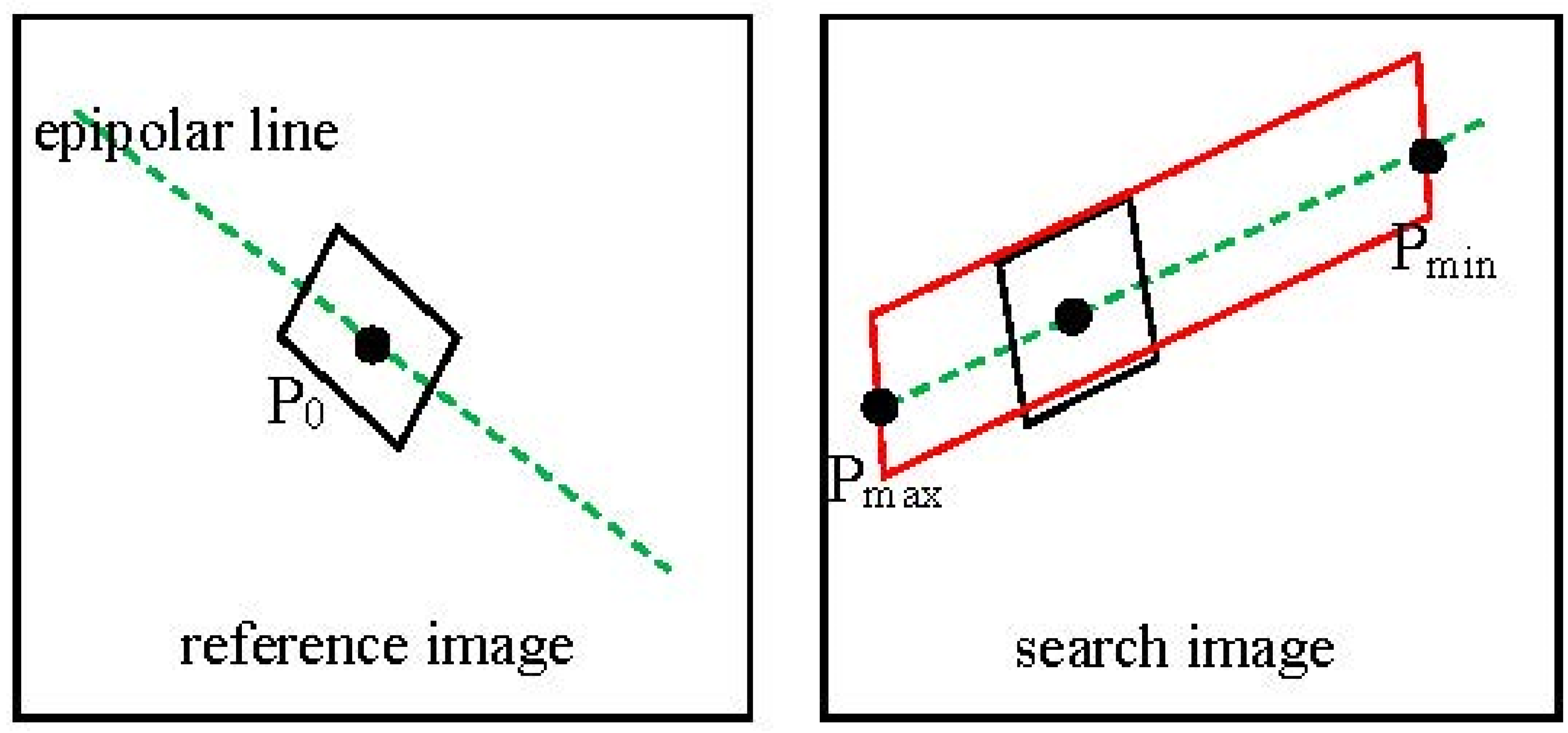
2.3.1. Multi-View Initial Feature-Matching

2.3.2. Matching Propagation Based on Self-Adaptive Patch

- (1)
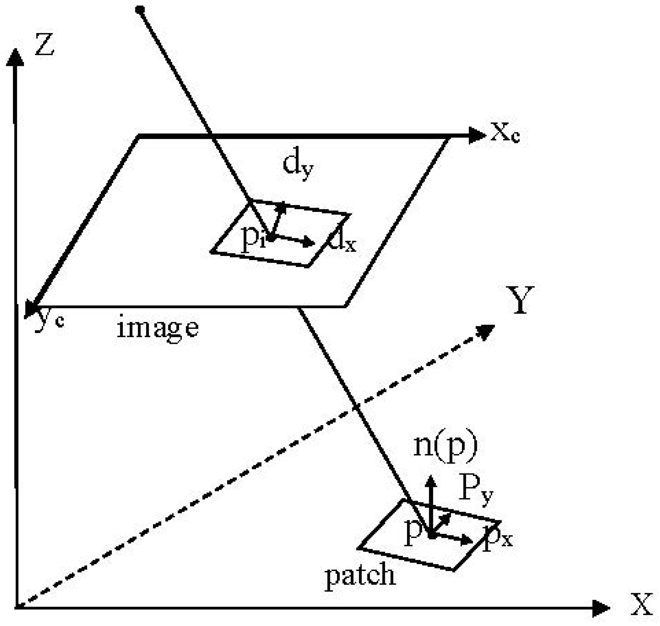
- Calculate the xyz-plane coordinate system of the patch, that is the x-axis is and the y-axis is , and the normal vector of the patch is seen as the z-axis (Figure 3). The patch center is considered the origin of the xyz-plane coordinate system of the patch. The y-axis is the vector that is perpendicular to the normal vector and the Xc-axis of the image space coordinate system; thus, . The x-axis is the vector that is perpendicular to the y-axis and the normal vector ; thus, . Then, and are normalized to the unit vector.
- (2)
- Calculate the ground resolution of the image as follows:where represents the distance between the patch center and the projection center of the image, represents the focal length, represents the angle between the light through the patch center and the normal vector of the patch, and actually represents the corresponding distance in the direction of for one pixel in the image.
- (3)
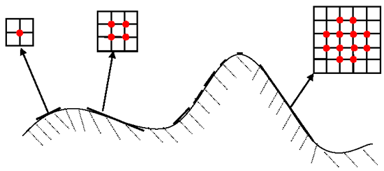
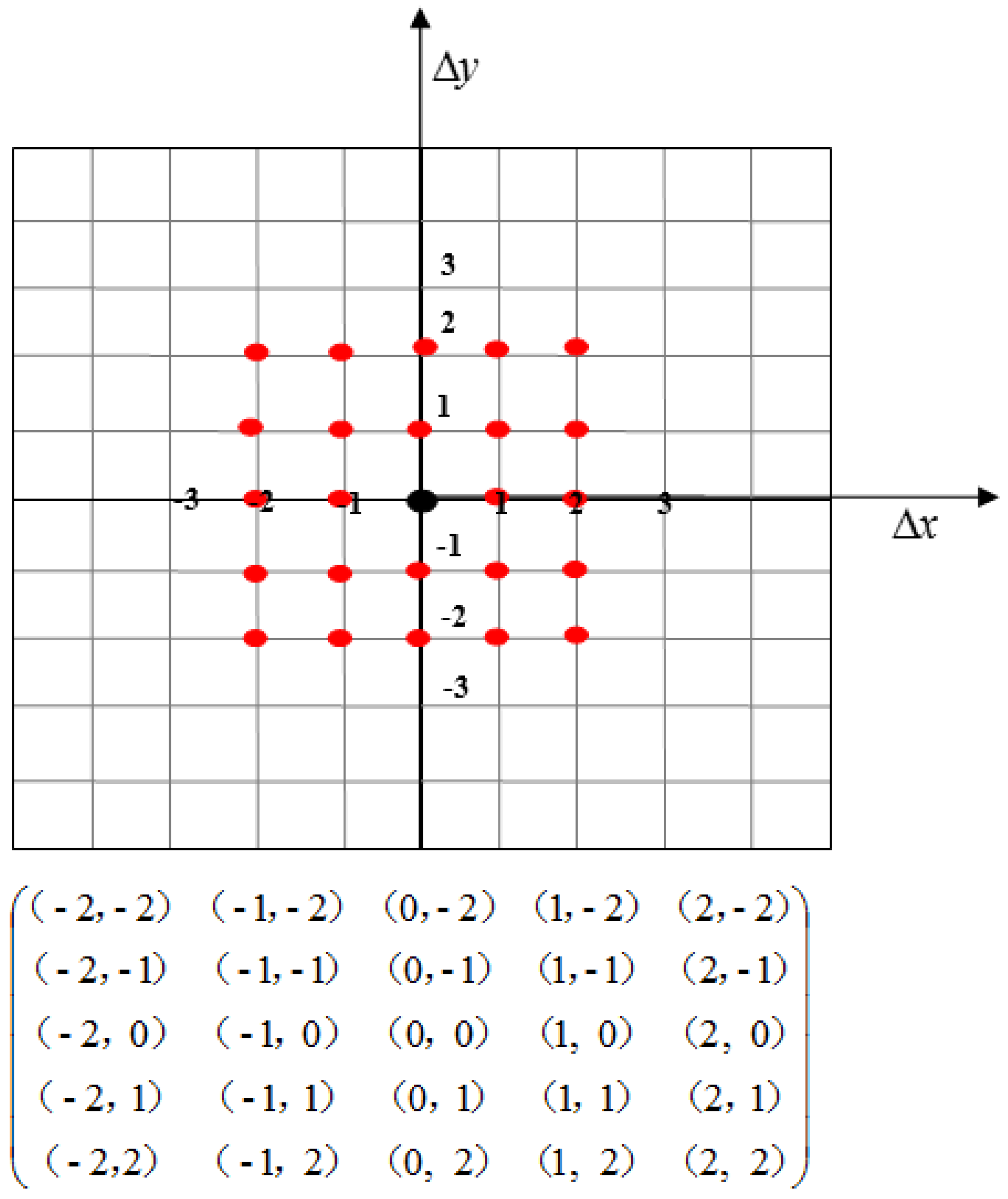
- Suppose a new point’s plane coordinate in the patch plane coordinate system is . The plane coordinates of the new points in the patch plane coordinate system are as shown in Figure 4. To ensure matching accuracy, the spread size is in the range of (the patch size is ) when the patch center is considered the origin of the patch plane coordinate system.


- (4)
- Calculate the XYZ-coordinate of the new point in the object space coordinate system. Suppose a (3D) new point is and the patch center is . We calculate the XYZ-coordinate of the new point as follows:
2.3.3. The Strategy of Matching Propagation
- (1)
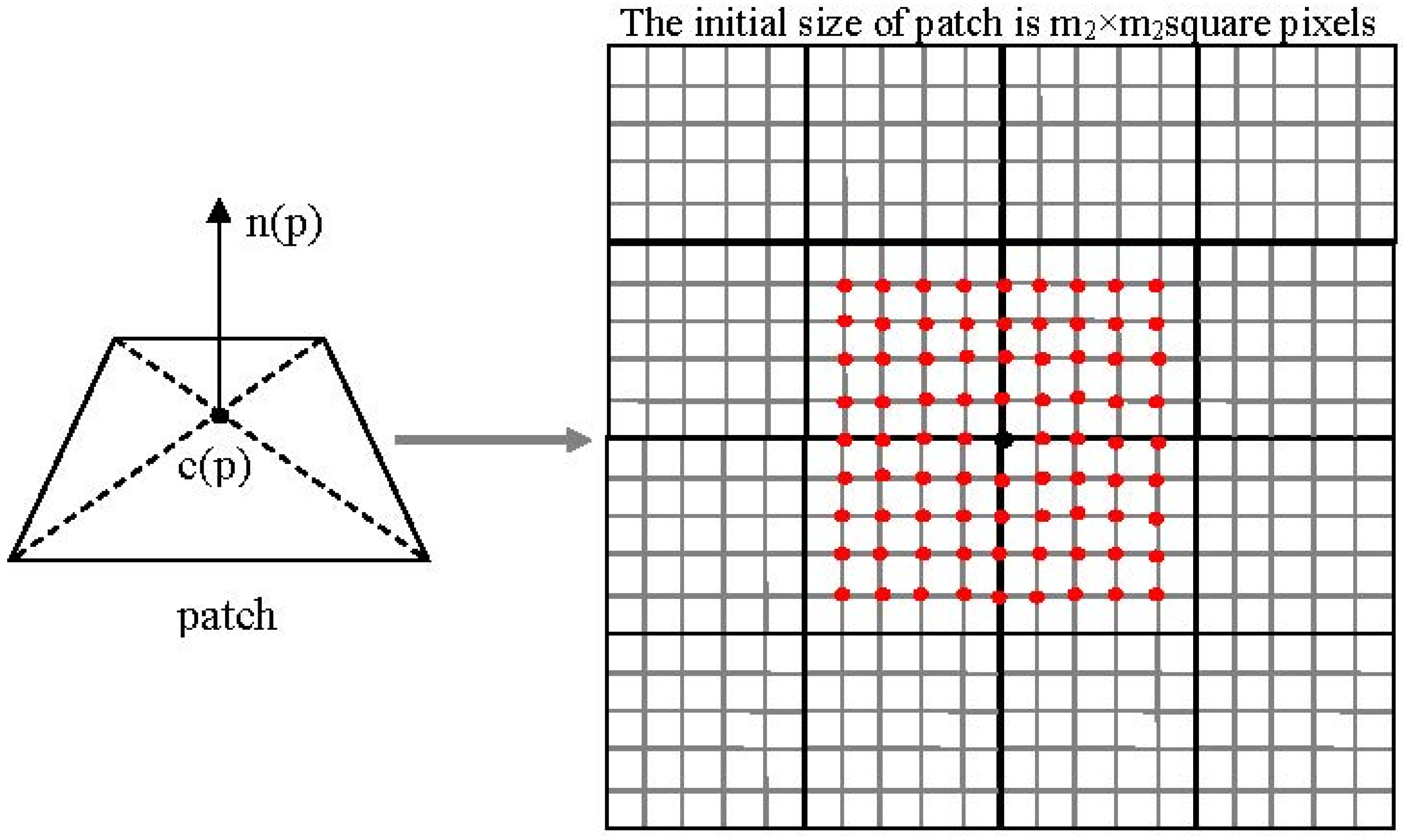
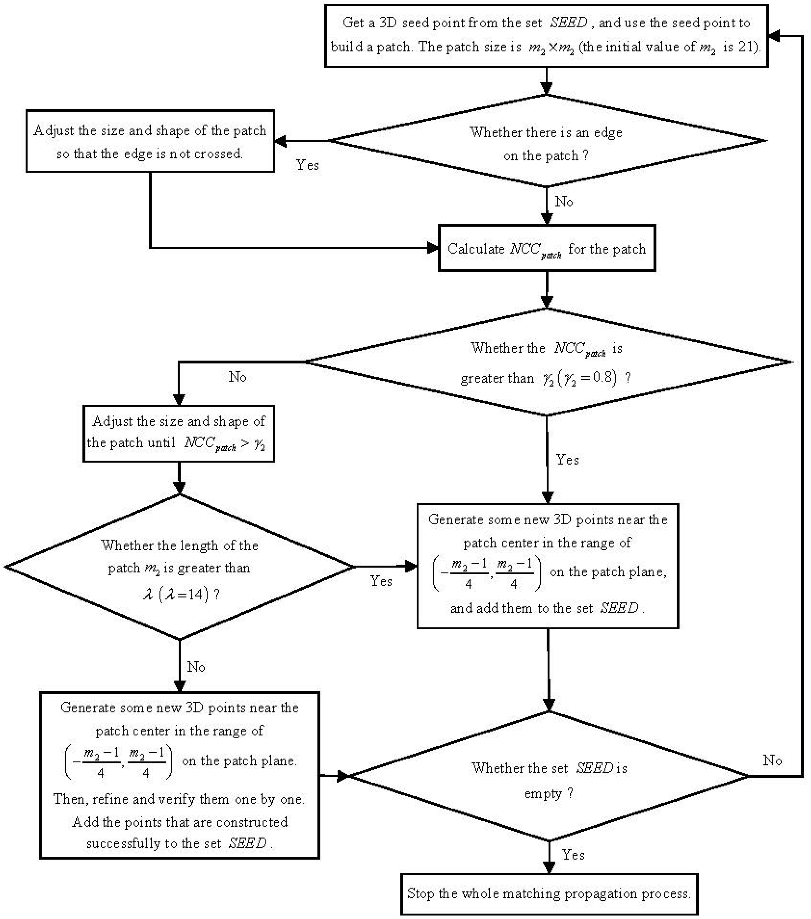
- Get a 3D seed point from the initial feature-matching set , and build a patch by using that point as the patch center. The initial size of the patch should ensure that the projection of the patch onto the reference image is of size square pixels. In this paper, is also denoted as the length of the patch, and the initial value of is 21. However, if the set becomes empty, stop the whole matching propagation process.
- (2)
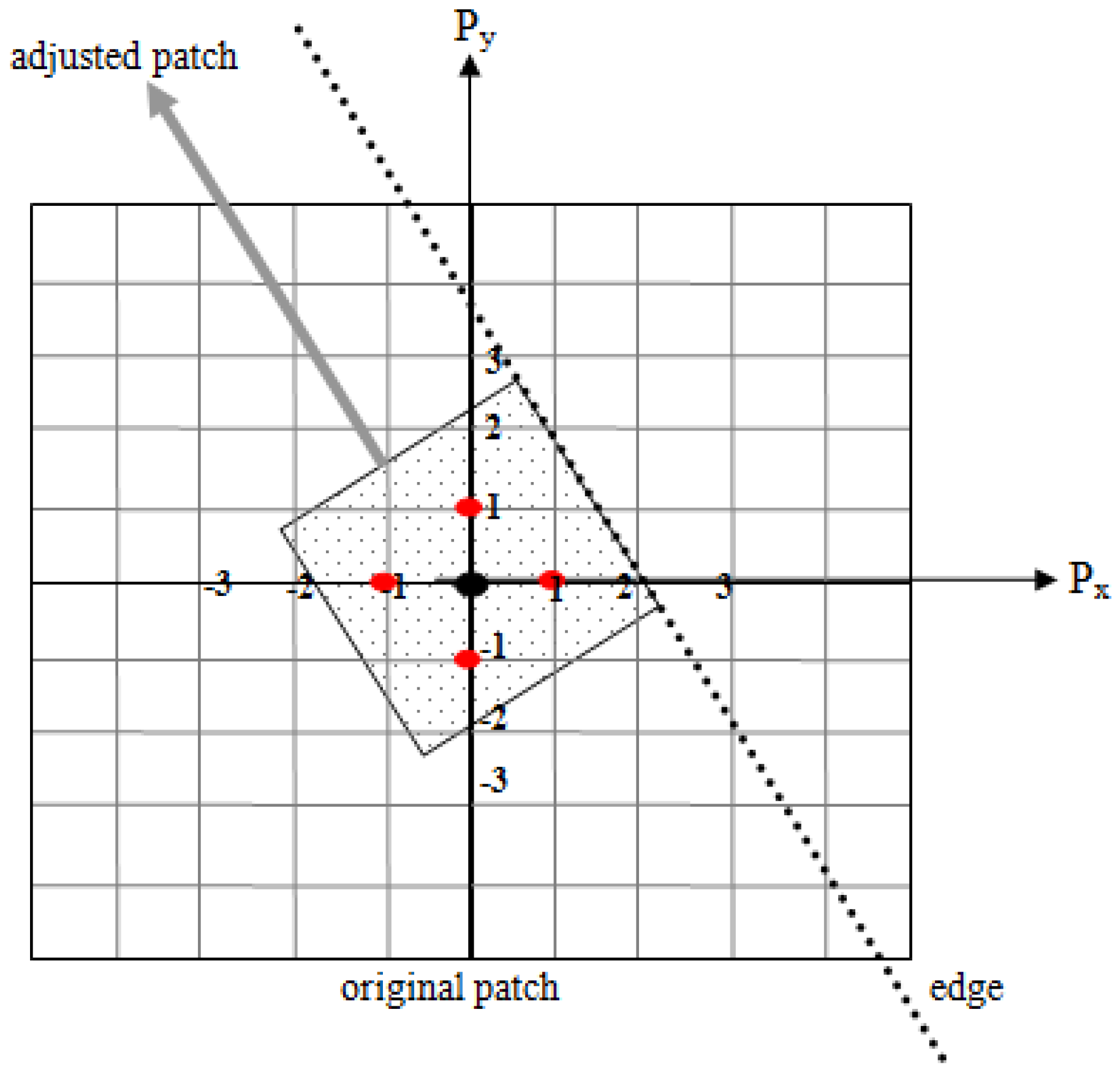
- If the patch does not contain any edge points, go to step 3. Otherwise, adjust the size and shape of the patch so that the edge (we used the edge points to determine the edge) is not crossed. In Figure 7, the patch is partitioned into two parts by an edge. We need to build a new patch from the part that contains the center point. The center point of the new patch is unchanged, and the shape is a square. One edge of the new patch is parallel to the edge. Thus, the length of the patch decreased and the shape also changed. Finally, go to step 3.
- (3)
- Take the projection of the patch onto each of the images as the relevant window, and use Equation (1) to calculate the correlation coefficient between the reference image and each search image. Then, use Equation (2) to calculate the average value of the correlation coefficients .
- (4)
- If , the size of the patch needs to be adjusted; thus, go to step 5, or else generate some new 3D points near the patch center in the range of on the patch plane. Details are presented in Section 2.3.2. Here, we need to judge whether another point has already been generated in that place. The judging method is as follows: project the new point onto the target image; if there is another point in the image pixel of the new point, give up the newly generated point. Directly add the remaining new points to the set , and go to step 1.
- (5)
- From one direction (e.g., the right), shrink the patch once by two pixels and calculate the in the meantime. If the value of is increased, continue to shrink the size of the patch in the same direction; otherwise, change the direction (e.g., left, up and down) to shrink the patch. The process above continues until . However, if the process continues until , go to step 1. After finishing the size and shape adjustment process, if the length of the patch is greater than pixels, go to step 4, or else go to step 6).
- (6)
- Generate new 3D points near the patch center in the range of on the patch plane (if , the scope becomes ). Then, refine and verify them one by one. Add the points that are constructed successfully to the set , and go to step 1.
2.3.4. Image-Grouping
- (1)
- Calculate the position and the size of the associated area (footprint) of every image, that is the corresponding ground points’ XY-plane coordinates for the four corner points of the image.
- (2)
- Compute the minimum enclosing rectangle of the entire photographed area according to the footprints of all the images.
- (3)
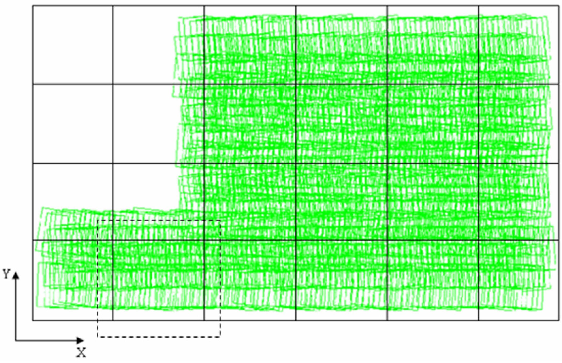
- Divide the minimum enclosing rectangle into blocks to ensure the number of images that are completely within each block is no more than but close to (Figure 8). Compute the footprint of each block, and enlarge the block. In Figure 8, the black dotted box represents the enlarged block, which is denoted by bigBlock.
- (4)
- According to the footprint of every image and the footprint of every bigBlock, take all the images belonging to one bigBlock as a group.
2.3.5. Group Matching and Merging the Results
3. Experiments and Results
3.1. Evaluation Index and Method
3.2. Experiments and Analysis
3.2.1. The Experimental Platform
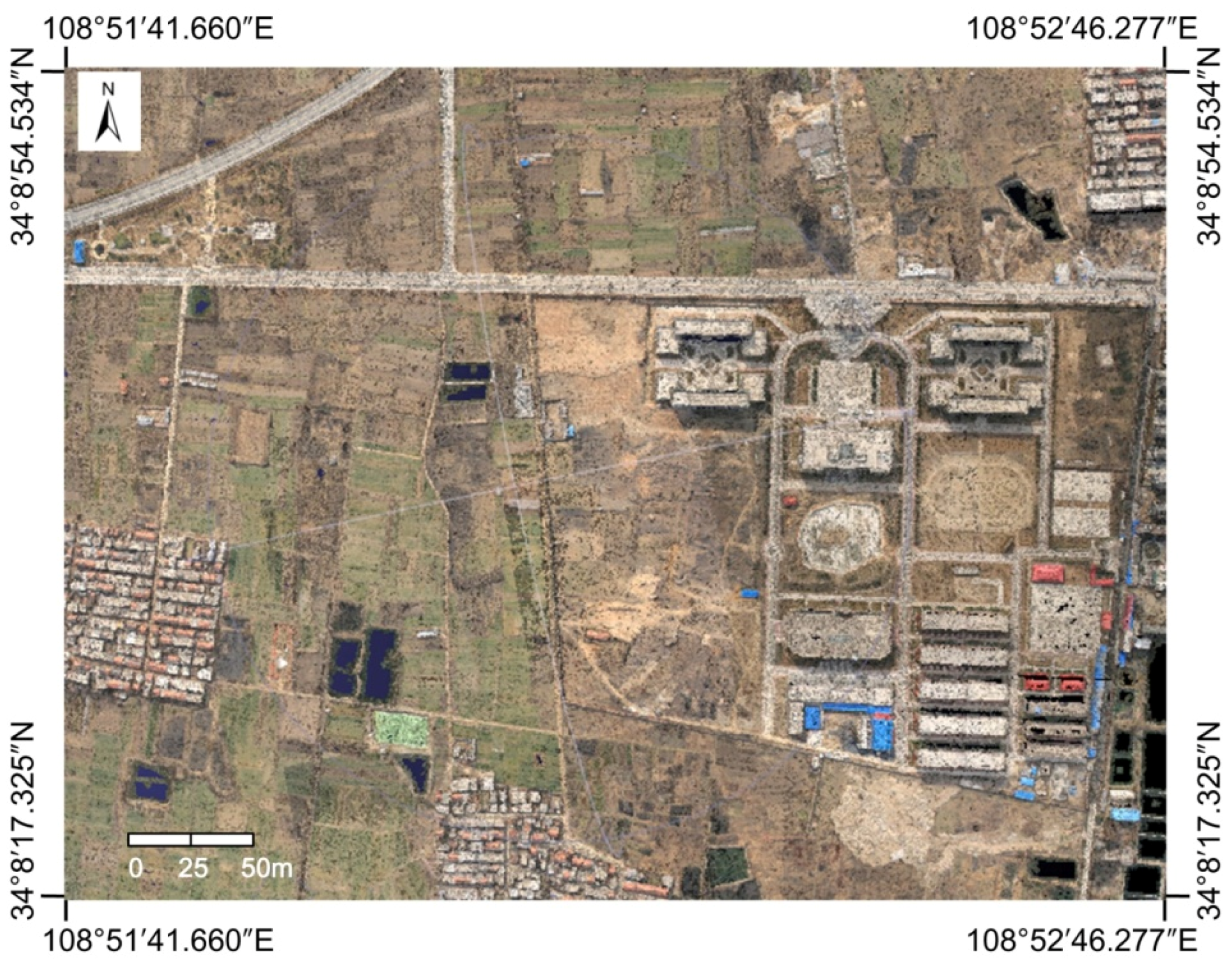
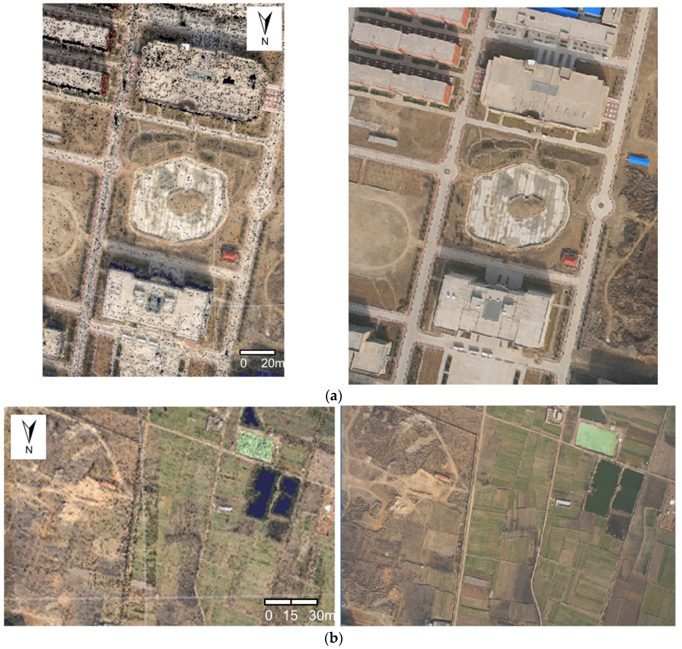
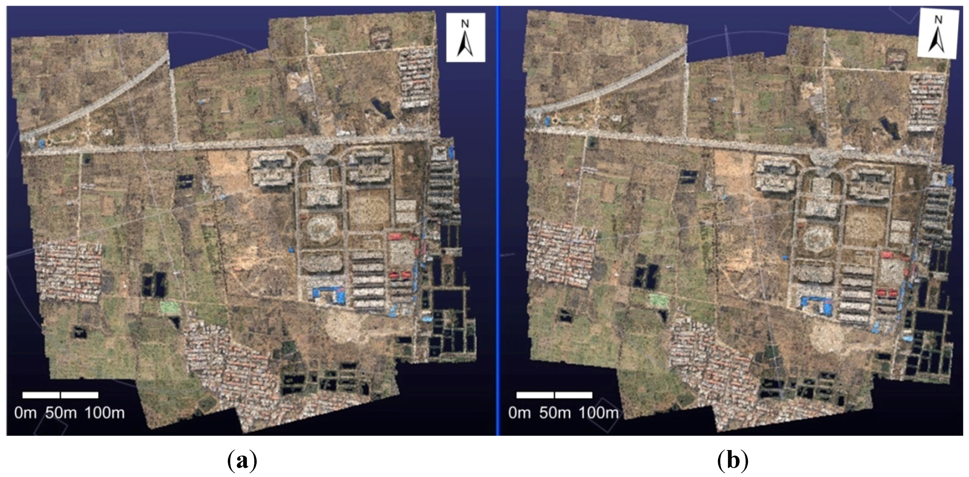
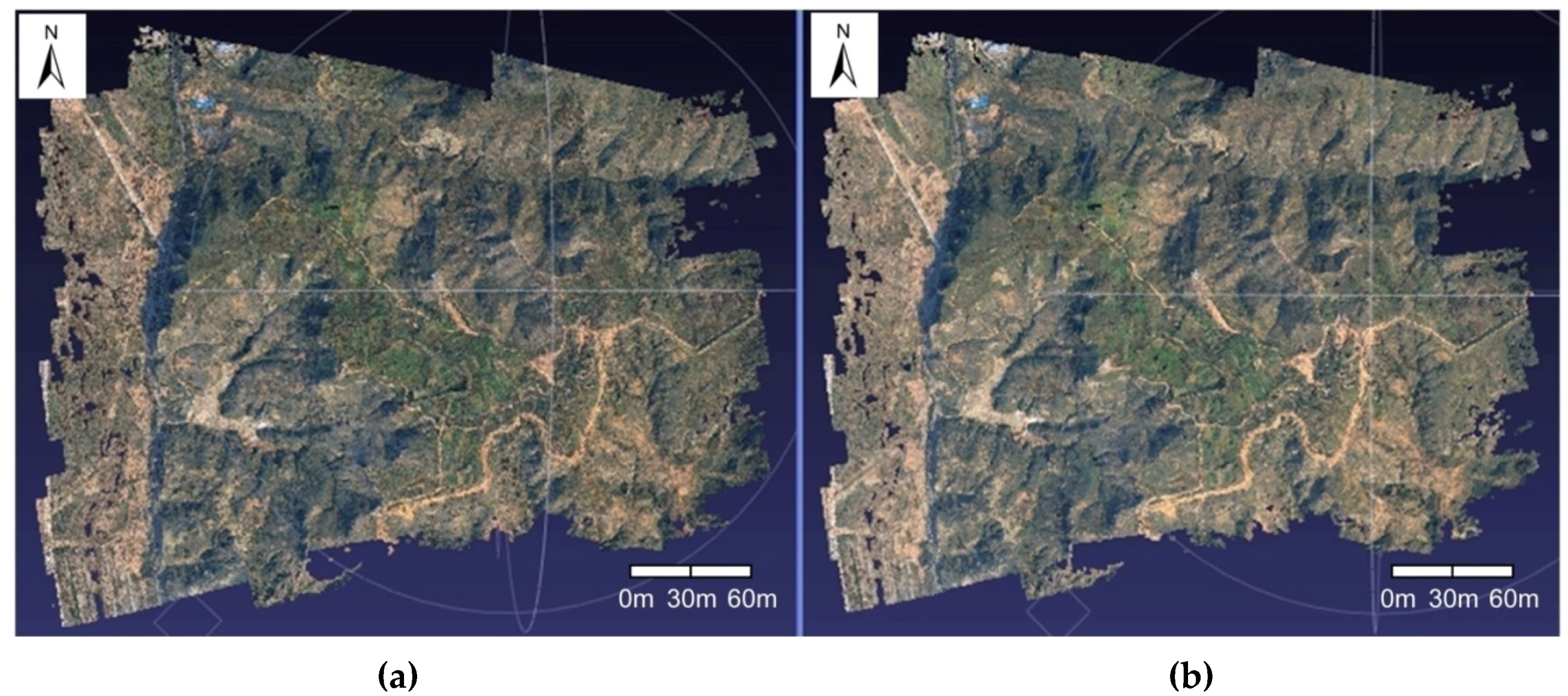
3.2.2. The First Dataset: Northwest University Campus, China

| Camera Name | CCD Size (mm × mm) | Image Resolution (pixels × pixels) | Pixel Size (μm) | Focal Length (mm) | Flying Height (m) | Ground Resolution (m) | Number of Images |
|---|---|---|---|---|---|---|---|
| Canon EOS 400D | 22.16 × 14.77 | 3888 × 2592 | 5.7 | 24 | 700 | 0.166 | 67 |

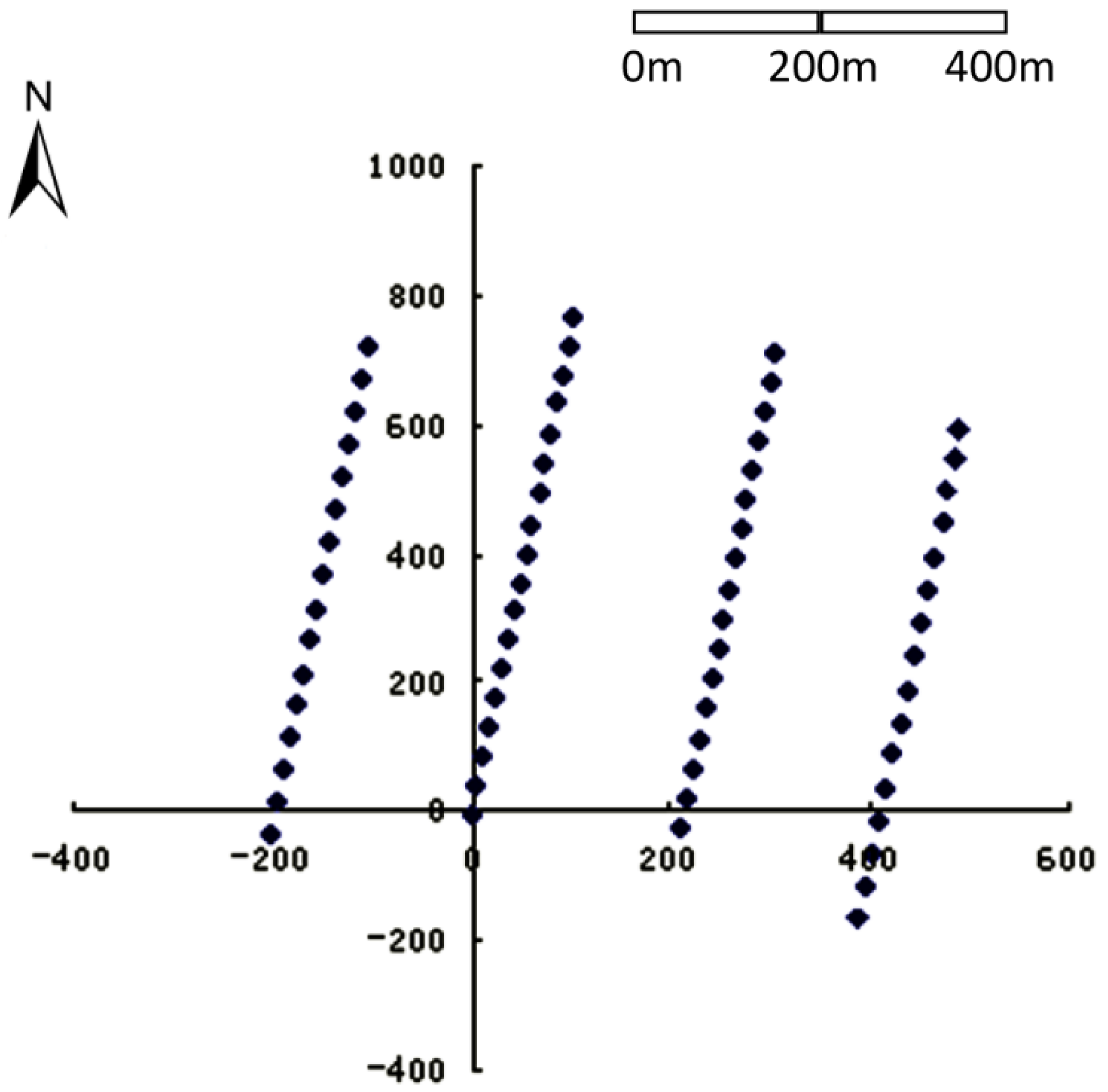
| Image Name | X (m) | Y (m) | Z (m) | φ (Degree) | ω (Degree) | κ (Degree) |
|---|---|---|---|---|---|---|
| IMG_0555 | −201.736 | −31.7532 | −1.35375 | −1.0234 | −0.44255 | 166.7002 |
| IMG_0554 | −194.482 | 17.90618 | −1.22801 | −0.71193 | −0.1569 | 166.2114 |
| IMG_0553 | −187.641 | 67.63342 | −0.87626 | 0.320481 | −0.03621 | 166.3385 |
| IMG_0552 | −180.965 | 116.052 | −0.61774 | 0.518773 | −0.87317 | 166.7509 |
| IMG_0551 | −174.434 | 166.2001 | −0.59227 | 0.454139 | −0.86679 | 167.2784 |
| IMG_0550 | −168.264 | 214.3878 | −0.79246 | −0.57551 | −0.67894 | 167.5912 |
| IMG_0549 | −162.096 | 265.1268 | −0.70428 | −1.08565 | −0.7456 | 167.166 |
| IMG_0548 | −156.002 | 314.2426 | −0.53393 | −1.40444 | −0.84598 | 166.5402 |
| IMG_0547 | −148.987 | 367.3003 | −0.30983 | −0.77136 | −0.86104 | 166.5097 |
| IMG_0546 | −142.152 | 417.2658 | −0.04708 | −0.38776 | −0.89084 | 166.5219 |
| IMG_0545 | −135.102 | 466.7365 | 0.507349 | −0.08542 | −0.09929 | 166.4838 |
| IMG_0544 | −128.322 | 520.032 | 1.246216 | −0.2938 | −0.41415 | 166.7157 |
| IMG_0543 | −121.833 | 569.8722 | 1.862483 | −0.20825 | −0.21687 | 167.1119 |
| Group | Image Number | Corresponding Image Name | Number of Images |
|---|---|---|---|
| 0 | 0 1 2 3 4 5 | IMG_1093~IMG_1089 | 6 |
| 1 | 6 7 8 9 10 11 | IMG_ 1087~IMG_1082 | 6 |
| 2 | 12 13 14 15 | IMG_1081~IMG_1078 | 4 |
| 3 | 16 17 18 19 20 21 | IMG_0102~IMG_0107 | 6 |
| 4 | 22 23 24 25 26 27 | IMG_0108~IMG_0113 | 6 |
| 5 | 28 29 30 31 32 | IMG_0114~IMG_0118 | 5 |
| 6 | 33 34 35 36 37 38 | IMG_0641~IMG_0646 | 6 |
| 7 | 39 40 41 42 43 44 | IMG_0647~IMG_0652 | 6 |
| 8 | 45 46 47 48 49 50 | IMG_0653~IMG_0658 | 6 |
| 9 | 51 52 53 54 55 56 | IMG_0555~IMG_0550 | 6 |
| 10 | 57 58 59 60 61 62 | IMG_0549~IMG_0544 | 6 |
| 11 | 63 64 65 66 | IMG_0543~IMG_0540 | 4 |


| Algorithm | RunTime (h:min:s) | Point Cloud Amount | Number of Images |
|---|---|---|---|
| IG-SAPMVS | 2:41:38 | 8526192 | 67 |
| PMVS | 4:8:30 | 7428720 | 67 |
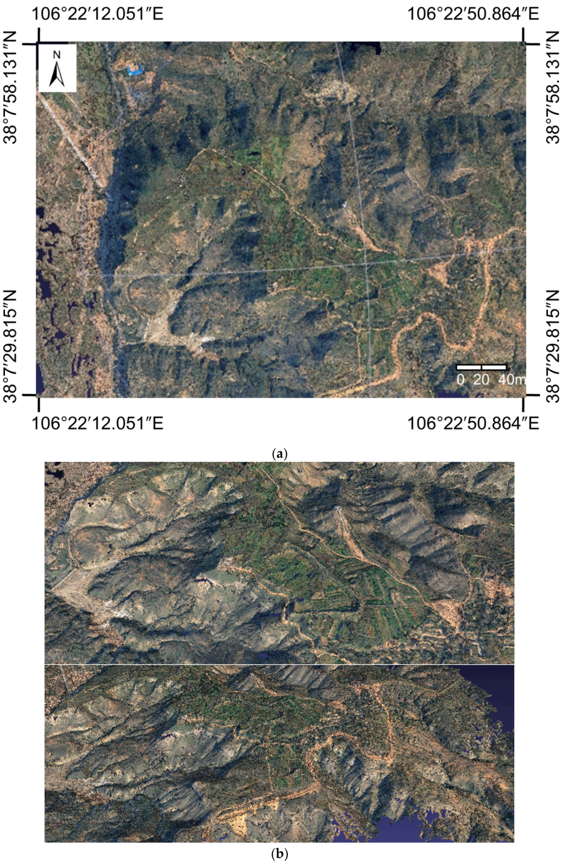
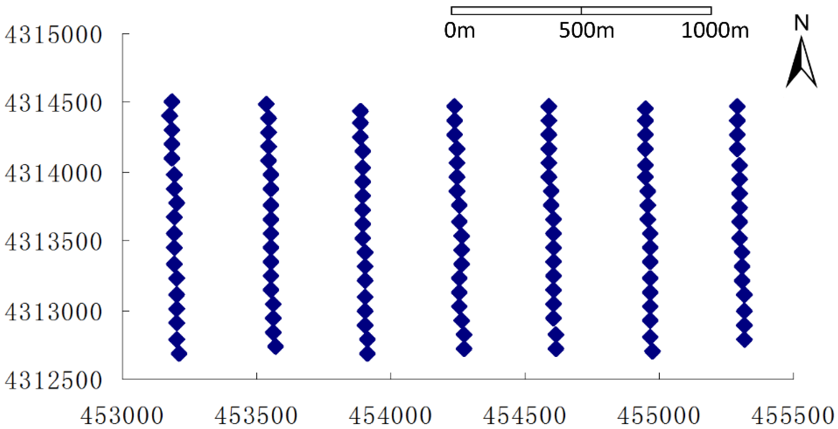
3.2.3. The Second Dataset: Remote Mountains
| Image Name | X (m) | Y (m) | Z (m) | φ (Degree) | ω (Degree) | κ (Degree) |
|---|---|---|---|---|---|---|
| IMG_0250 | 453208.9 | 4312689 | 1926.36 | 4.251745 | −2.30691 | 10.23632 |
| IMG_0251 | 453205.6 | 4312796 | 1926.462 | 2.852207 | −6.04494 | 10.94959 |
| IMG_0252 | 453200.6 | 4312900 | 1921.71 | 0.681977 | −7.93856 | 11.60872 |
| IMG_0253 | 453198.6 | 4313007 | 1920.499 | −0.01863 | −3.6135 | 8.714555 |
| IMG_0254 | 453198.7 | 4313117 | 1915.972 | 3.277204 | −6.38877 | 8.599633 |
| IMG_0255 | 453199.3 | 4313230 | 1910.448 | 6.64432 | −6.29777 | 8.965715 |
| IMG_0256 | 453196.7 | 4313341 | 1904.105 | 3.33602 | −6.5811 | 10.72329 |
| IMG_0257 | 453194.1 | 4313450 | 1903.386 | 1.594531 | −4.486 | 10.71933 |
| IMG_0258 | 453192.8 | 4313559 | 1902.593 | −4.04339 | −5.57166 | 8.112464 |
| IMG_0259 | 453194.9 | 4313667 | 1899.551 | 3.77633 | −2.96418 | 7.066141 |
| IMG_0260 | 453198.2 | 4313776 | 1899.075 | 7.240338 | −5.29839 | 8.254281 |
| IMG_0261 | 453196.6 | 4313882 | 1898.725 | 3.41796 | −1.02482 | 10.90049 |
| IMG_0262 | 453193.1 | 4313986 | 1895.928 | 3.000324 | −5.9483 | 12.35882 |
| IMG_0263 | 453185.4 | 4314095 | 1896.413 | 1.532879 | −4.00544 | 11.27756 |
| IMG_0264 | 453184 | 4314196 | 1895.204 | 4.379199 | −2.4512 | 11.95034 |

| Algorithm | RunTime (h:min:s) | Point Cloud Amount | Number of Images |
|---|---|---|---|
| IG-SAPMVS | 4:36:5 | 12509202 | 125 |
| PMVS | 15:48:11 | 8953228 | 125 |
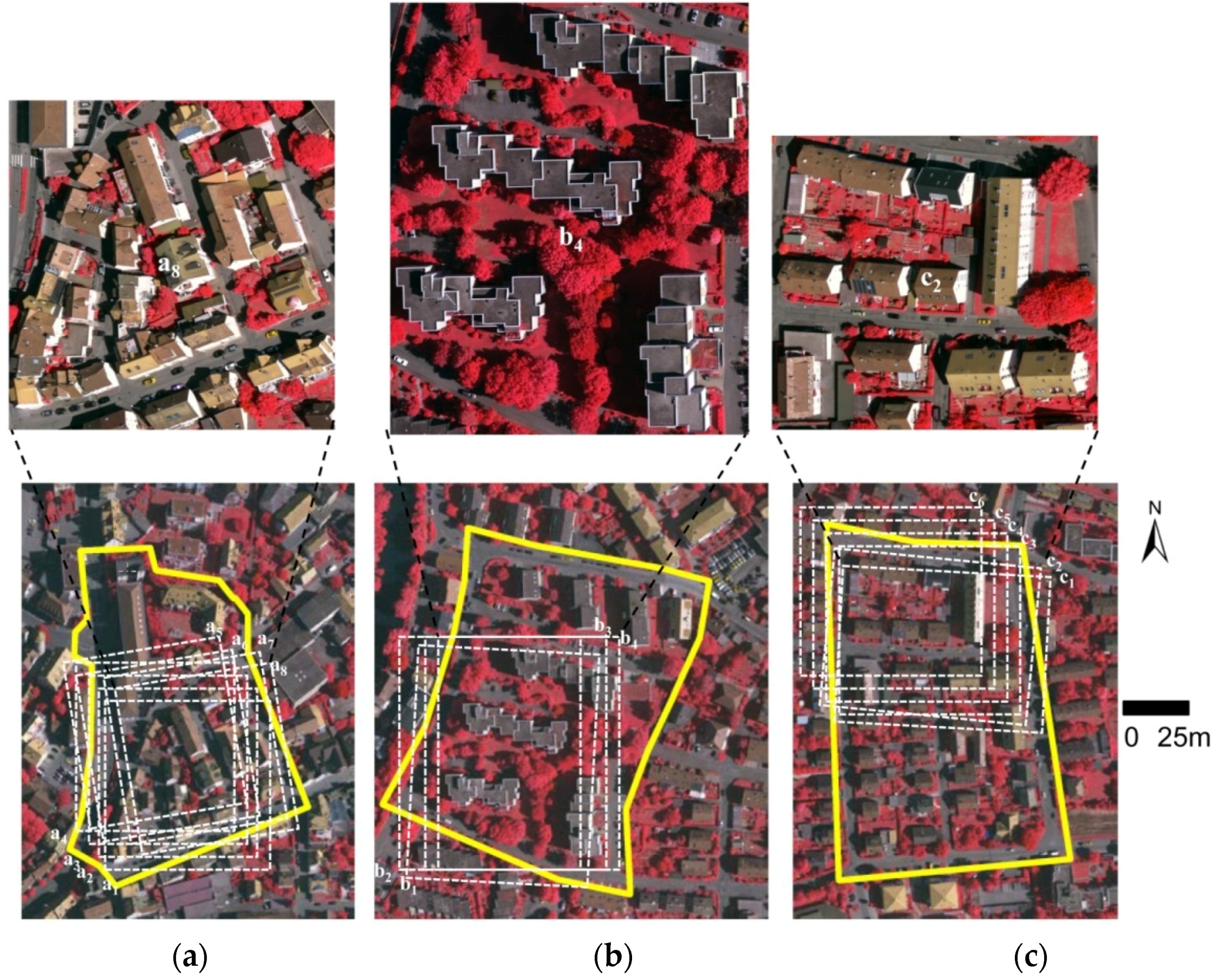
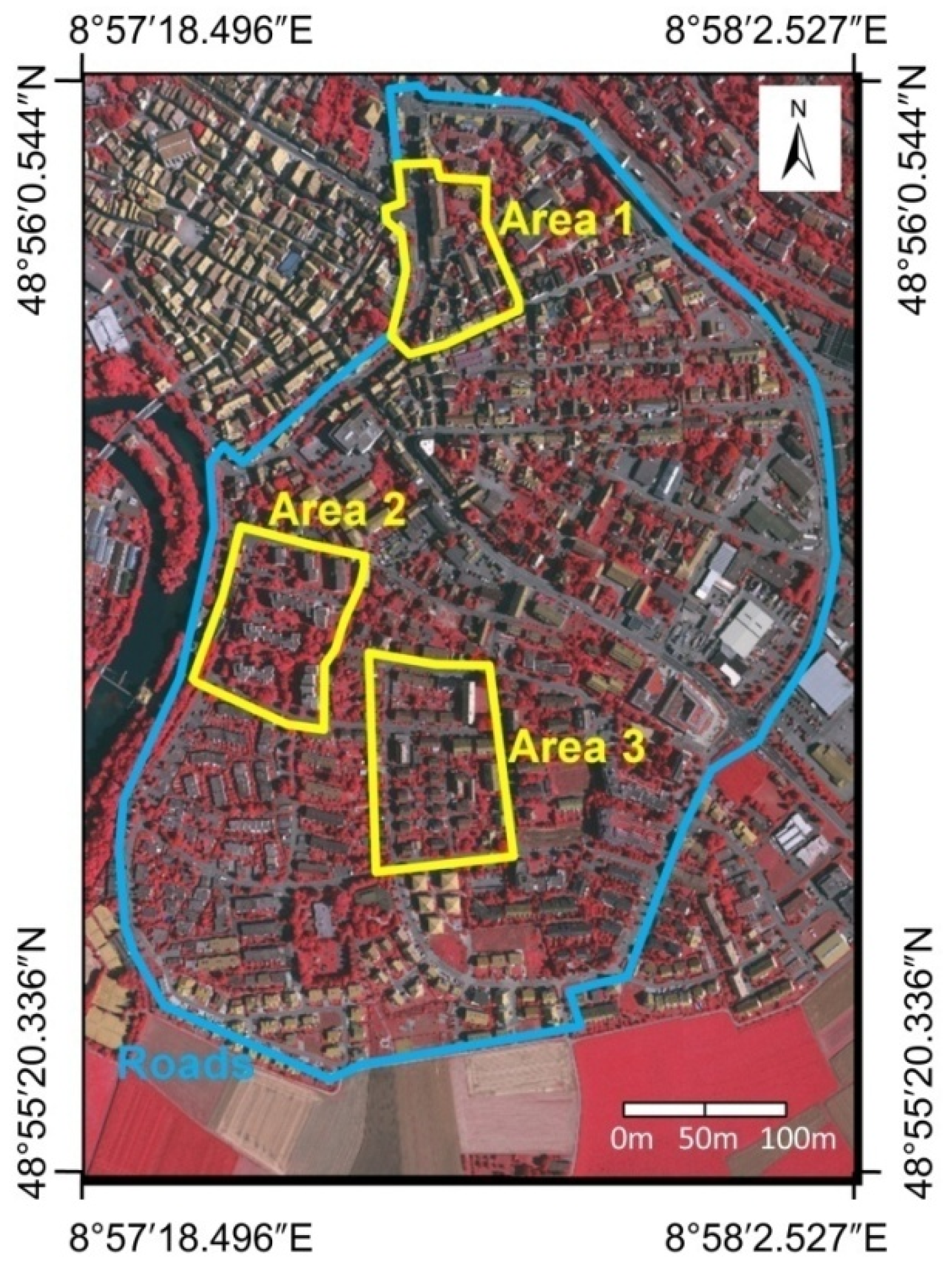
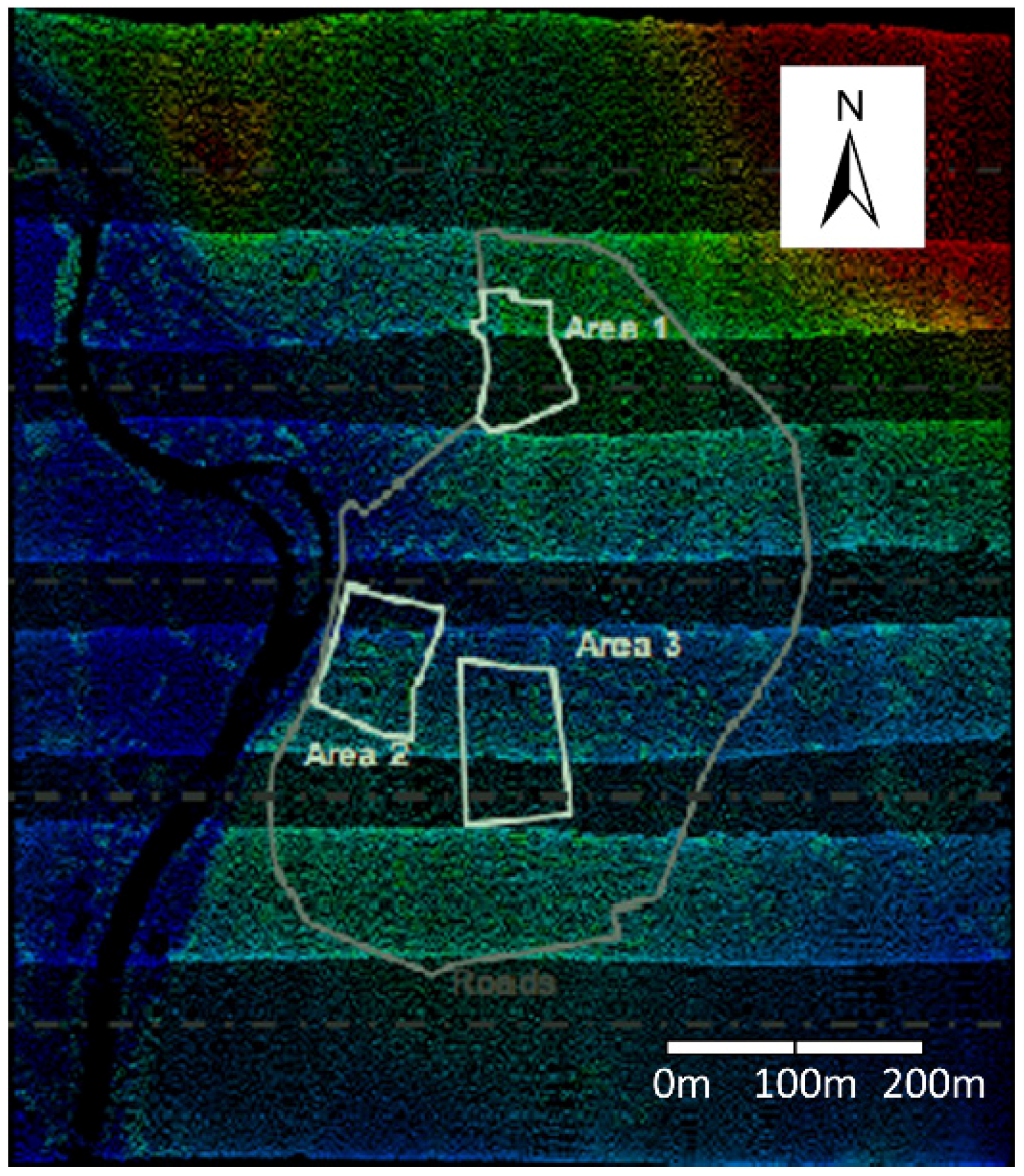
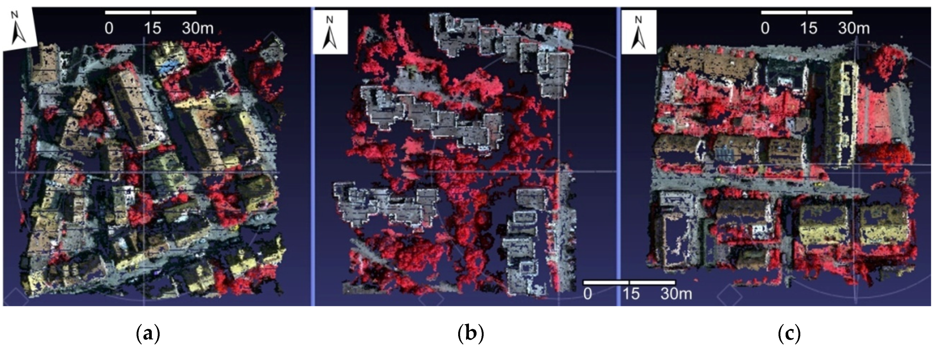
3.2.4. The Third Dataset: Vaihingen, Germany
- •
- Area 1 “Inner City”: This test area is situated in the center of the city of Vaihingen. It is characterized by dense development consisting of historic buildings with rather complex shapes, but there are also some trees (Figure 17a).
- •
- Area 2 “High Riser”: This area is characterized by a few high-rise residential buildings that are surrounded by trees (Figure 17b).
- •
- Area 3 “Residential Area”: This is a purely residential area with small detached houses (Figure 17c).

| Image Name | X (m) | Y (m) | Z (m) | ω (Degree) | ϕ (Degree) | κ (Degree) |
|---|---|---|---|---|---|---|
| 10030060.tif | 496803.043 | 5420298.566 | 1163.983 | 2.50674 | 0.73802 | 199.32970 |
| 10030061.tif | 497049.238 | 5420301.525 | 1163.806 | 2.05968 | 0.67409 | 199.23470 |
| 10030062.tif | 497294.288 | 5420301.839 | 1163.759 | 1.97825 | 0.51201 | 198.84290 |
| 10030063.tif | 497539.821 | 5420299.469 | 1164.423 | 1.40457 | 0.38326 | 198.88310 |
| 10040081.tif | 496558.488 | 5419884.008 | 1181.985 | −0.87093 | 0.36520 | −199.20110 |
| 10040082.tif | 496804.479 | 5419882.183 | 1183.373 | −0.26935 | −0.63812 | −198.97290 |
| 10040083.tif | 497048.699 | 5419882.847 | 1184.616 | 0.34834 | −0.40178 | −199.44720 |
| 10040084.tif | 497296.587 | 5419884.550 | 1185.010 | 0.81501 | −0.53024 | −199.35600 |
| 10040085.tif | 497540.779 | 5419886.806 | 1184.876 | 1.38534 | −0.46333 | −199.85010 |
| 10050103.tif | 496573.389 | 5419477.807 | 1161.431 | −0.48280 | −0.03105 | −0.23869 |
| 10050104.tif | 496817.972 | 5419476.832 | 1161.406 | −0.65210 | −0.06311 | −0.17326 |
| 10050105.tif | 497064.985 | 5419476.630 | 1159.940 | −0.74655 | 0.11683 | −0.09710 |
| 10050106.tif | 497312.996 | 5419477.065 | 1158.888 | −0.53451 | −0.19025 | −0.13489 |
| 10050107.tif | 497555.389 | 5419477.724 | 1158.655 | −0.55312 | −0.12844 | −0.13636 |
| 10250130.tif | 497622.784 | 5420189.950 | 1180.494 | 0.09448 | 3.41227 | −101.14170 |
| 10250131.tif | 497630.734 | 5419944.364 | 1181.015 | 0.61065 | 2.54420 | −97.84478 |
| 10250132.tif | 497633.024 | 5419698.973 | 1179.964 | 1.27053 | 1.62793 | −97.23292 |
| 10250133.tif | 497628.317 | 5419452.807 | 1179.237 | 0.90688 | 0.83308 | −98.72504 |
| 10250134.tif | 497620.954 | 5419207.621 | 1178.201 | 0.17675 | 1.27920 | −101.86160 |
| 10250135.tif | 497617.307 | 5418960.618 | 1176.629 | 0.22019 | 1.47729 | −101.55860 |
| Experiment Area | Number of Images (Image Pixel Resolution) | Point Amount | Average Distance between Points | RunTime (min:s) |
|---|---|---|---|---|
| Area 1: “Inner City” | 8 (1200*1200) | 253125 | 16 cm | 11:33 |
| Area 2: “High Riser” | 4 (1200*1600) | 220073 | 16 cm | 6:30 |
| Area 3: “Residential Area” | 6 (1400*1300) | 259637 | 16 cm | 9:46 |
| (a) | ||||
| Experiment Area | Checkpoint Amount | RMSE(m) | Max(m) | Percentage of Errors within 1 m |
| Area 1: “Inner City” | 245752 | 2.180527 | 20.410379 | 66.7% |
| Area 2: “High Riser” | 213679 | 4.032463 | 30.742815 | 46.1% |
| Area 3: “Residential Area” | 252568 | 2.349705 | 18.903685 | 74.1% |
| (b) | ||||
| Experiment Area | Checkpoint Amount | RMSE(m) | Max(m) | Percentage of Errors within 1 m |
| Area 1: “Inner City” | 253125 | 2.164632 | 20.307628 | 66.8% |
| Area 2: “High Riser” | 220073 | 3.950138 | 29.812880 | 46.4% |
| Area 3: “Residential Area” | 259637 | 2.328481 | 18.713413 | 74.2% |
| (a) | ||||
| Experiment Area | Point Amount | Checkpoint Amount | RMSE(m) | Percentage of Errors within 1 m |
| Area 1: “Inner City” | 245752 | 243179 | 1.312648 | 67.5% |
| Area 2: “High Riser” | 213679 | 212151 | 3.402339 | 46.5% |
| Area 3: “Residential Area” | 252568 | 250463 | 1.587426 | 74.7% |
| (b) | ||||
| Experiment Area | Point Amount | Checkpoint Amount | RMSE(m) | Percentage of Errors within 1 m |
| Area 1: “Inner City” | 253125 | 250488 | 1.301095 | 67.5% |
| Area 2: “High Riser” | 220073 | 218508 | 3.352631 | 46.7% |
| Area 3: “Residential Area” | 259637 | 257470 | 1.571167 | 74.8% |
| (a) | ||||
| Experiment Area | Point Amount | Checkpoint Amount | RMSE (m) | Percentage of Errors within 1 m |
| Area 1: “Inner City” | 245752 | 240826 | 0.880695 | 68.2% |
| Area 2: “High Riser” | 213679 | 173487 | 1.351428 | 57.1% |
| Area 3: “Residential Area” | 252568 | 248728 | 0.898527 | 75.3% |
| (b) | ||||
| Experiment Area | Point Amount | Checkpoint Amount | RMSE (m) | Percentage of Errors within 1 m |
| Area 1: “Inner City” | 253125 | 248113 | 0.870425 | 68.1% |
| Area 2: “High Riser” | 220073 | 178565 | 1.316283 | 57.2% |
| Area 3: “Residential Area” | 259637 | 255674 | 0.886161 | 75.3% |
3.2.5. Discussion
- (1)
- The proposed multi-view stereo-matching algorithm based on matching control strategies suitable for multiple UAV imagery and the self-adaptive patch can address the UAV image data with different texture features effectively. The obtained dense point cloud has a realistic effect, and the precision is equal to that of the PMVS algorithm.
- (2)
- Due to the image-grouping strategy, the proposed algorithm can handle a large amount of data on a typical computer and is, to a large degree, not restricted by the memory of the computer.
- (3)
- The proposed matching propagation method based on the self-adaptive patch is superior to that of the state-of-the-art PMVS algorithm in terms of the processing efficiency, and has, to some extent, improved the accuracy of the multi-view stereo-matching algorithm by the self-adaptive spread patch sizes according to terrain relief, e.g., a small spread patch size for large relief terrain, and avoiding crossing the terrain edge, i.e., the fracture line.
- (1)
- The accuracy and completeness of the proposed algorithm.
- (2)
- The accuracy evaluation method of the proposed algorithm.
4. Conclusions
Acknowledgments
Author Contributions
Conflicts of Interest
References
- Lin, Z.; Su, G.; Xie, F. UAV borne low altitude photogrammetry system. Int. Arch. Photogramm. Remote Sens. Spat. Inf. Sci. 2012, XXXIX-B1, 415–423. [Google Scholar] [CrossRef]
- Tong, X.; Liu, X.; Chen, P.; Liu, S.; Luan, K.; Li, L.; Liu, S.; Liu, X.; Xie, H.; Jin, Y.; et al. Integration of UAV-based photogrammetry and terrestrial laser scanning for the three-dimensional mapping and monitoring of open-pit mine areas. Remote Sens. 2015, 7, 6635–6662. [Google Scholar] [CrossRef]
- Colomina, I.; Molina, P. Unmanned aerial systems for photogrammetry and remote sensing: A review. ISPRS J. Photogramm. Remote Sens. 2014, 92, 79–97. [Google Scholar] [CrossRef]
- Ahmad, A. Digital mapping using low altitude UAV. Pertan. J. Sci. Technol. 2011, 19, 51–58. [Google Scholar]
- Eisenbeiss, H. UAV Photogrammetry. Ph.D. Thesis, Swiss Federal Institute of Technology Zurich, Zurich, Switzerland, 2009. [Google Scholar]
- Udin, W.S.; Ahmad, A. Large scale mapping using digital aerial imagery of unmanned aerial vehicle. Int. J. Sci. Eng. Res. 2012, 3, 1–6. [Google Scholar]
- Remondino, F.; Barazzetti, L.; Nex, F.; Scaioni, M.; Sarazzi, D. UAV photogrammetry for mapping and 3d modeling–current status and future perspectives. In Proceedings of the International Conference on Unmanned Aerial Vehicle in Geomatics (UAV-g), Zurich, Switzerland, 14–16 September 2011; pp. 1–7.
- Bachmann, F.; Herbst, R.; Gebbers, R.; Hafner, V.V. Micro UAV based georeferenced orthophoto generation in VIS+ NIR for precision agriculture. Int. Arch. Photogramm. Remote Sens. Spat. Inf. Sci. 2013, XL-1/W2, 11–16. [Google Scholar] [CrossRef]
- Lin, Y.; Saripalli, S. Road detection from aerial imagery. In Proceedings of the 2012 IEEE International Conference on Robotics and Automation (ICRA), Saint Paul, MN, USA, 14–18 May 2012; pp. 3588–3593.
- Bendea, H.; Chiabrando, F.; Tonolo, F.G.; Marenchino, D. Mapping of archaeological areas using a low-cost UAV. In Proceedings of the XXI International CIPA Symposium, Athens, Greece, 1–6 October 2007.
- Coifman, B.; McCord, M.; Mishalani, R.G.; Iswalt, M.; Ji, Y. Roadway traffic monitoring from an unmanned aerial vehicle. IEE Proc. Intell. Trans. Syst. 2006, 153, 11–20. [Google Scholar] [CrossRef]
- Wang, J.; Lin, Z.; Li, C. Reconstruction of buildings from a single UAV image. In Proceedings of the International Society for Photogrammetry and Remote Sensing Congress, Istanbul, Turkey, 12–23 July 2004; pp. 100–103.
- Quaritsch, M.; Kuschnig, R.; Hellwagner, H.; Rinner, B.; Adria, A.; Klagenfurt, U. Fast aerial image acquisition and mosaicking for emergency response operations by collaborative UAVs. In Proceedings of the International ISCRAM Conference, Lisbon, Portugal, 8–11 May 2011; pp. 1–5.
- Lin, Z. UAV for mapping—Low altitude photogrammetry survey. Int. Arch. Photogramm. Remote Sens. Spat. Inf. Sci. 2008, XXXVII, 1183–1186. [Google Scholar]
- Zhang, Y.; Xiong, J.; Hao, L. Photogrammetric processing of low-altitude images acquired by unpiloted aerial vehicles. Photogramm. Rec. 2011, 26, 190–211. [Google Scholar] [CrossRef]
- Ai, M.; Hu, Q.; Li, J.; Wang, M.; Yuan, H.; Wang, S. A robust photogrammetric processing method of low-altitude UAV images. Remote Sens. 2015, 7, 2302–2333. [Google Scholar] [CrossRef]
- Seitz, S.M.; Curless, B.; Diebel, J.; Scharstein, D.; Szeliski, R. A comparison and evaluation of multi-view stereo reconstruction algorithms. In Proceedings of the 2006 IEEE Computer Society Conference on Computer Vision and Pattern Recognition (CVPR’06), New York, NY, USA, 17–22 June 2006; pp. 519–528.
- Furukawa, Y.; Ponce, J. Accurate, dense, and robust multi-view stereopsis. IEEE Trans. Pattern Anal. Mach. Intell. 2010, 32, 1362–1376. [Google Scholar] [CrossRef] [PubMed]
- Faugeras, O.; Keriven, R. Variational principles, surface evolution, pdes, level set methods, and the stereo problem. IEEE Trans. Image Process. 1998, 7, 336–344. [Google Scholar] [CrossRef] [PubMed]
- Pons, J.P.; Keriven, R.; Faugeras, O. Multi-view stereo reconstruction and scene flow estimation with a global image-based matching score. Int. J. Comput. Vis. 2007, 72, 179–193. [Google Scholar] [CrossRef]
- Tran, S.; Davis, L. 3d surface reconstruction using graph cuts with surface constraints. In Proceedings of the European Conf. Computer Vision (ECCV 2006), Graz, Austria, 7–13 May 2006; pp. 219–231.
- Vogiatzis, G.; Torr, P.H.S.; Cipolla, R. Multi-view stereo via volumetric graph-cuts. In Proceedings of the 2005 IEEE Computer Society Conference on Computer Vision and Pattern Recognition (CVPR 2005), San Diego, CA, USA, 20–25 June 2005; pp. 391–398.
- Hornung, A.; Kobbelt, L. Hierarchical volumetric multi-view stereo reconstruction of manifold surfaces based on dual graph embedding. In Proceedings of the 2006 IEEE Computer Society Conference on Computer Vision and Pattern Recognition (CVPR 2006), New York, NY, USA, 17–22 June 2006; pp. 503–510.
- Sinha, S.N.; Mordohai, P.; Pollefeys, M. Multi-view stereo via graph cuts on the dual of an adaptive tetrahedral mesh. In Proceedings of the 11th IEEE International Conference on Computer Vision (ICCV 2007), Rio de Janeiro, Brazil, 14–21 October 2007; pp. 1–8.
- Kolmogorov, V.; Zabih, R. Multi-camera scene reconstruction via graph cuts. In Proceedings of the 7th European Conference on Computer Vision (ECCV 2002), Copenhagen, Denmark, 28–31 May 2002; pp. 82–96.
- Vogiatzis, G.; Hernandez, C.; Torr, P.H.S.; Cipolla, R. Multi-view stereo via volumetric graph-cuts and occlusion robust photo-consistency. IEEE Trans. Pattern Anal. Mach. Intell. 2007, 29, 2241–2246. [Google Scholar] [CrossRef] [PubMed]
- Esteban, C.H.; Schmitt, F. Silhouette and stereo fusion for 3d object modeling. In Proceedings of the Fourth International Conference on 3-D Digital Imaging and Modeling (3DIM 2003), Banff, AB, Canada, 6–10 October 2003; pp. 46–53.
- Zaharescu, A.; Boyer, E.; Horaud, R. Transformesh: A topology-adaptive mesh-based approach to surface evolution. In Proceedings of the 8th Asian Conference on Computer Vision (ACCV 2007), Tokyo, Japan, 18–22 November 2007; pp. 166–175.
- Furukawa, Y.; Ponce, J. Carved visual hulls for image-based modeling. Int. J. Comput. Vis. 2009, 81, 53–67. [Google Scholar] [CrossRef]
- Baumgart, B.G. Geometric Modeling for Computer Vision. PhD Thesis, Stanford University, Stanford, CA, USA, 1974. [Google Scholar]
- Laurentini, A. The visual hull concept for silhouette-based image understanding. IEEE Trans. Pattern Anal. Mach. Intell. 1994, 16, 150–162. [Google Scholar] [CrossRef]
- Strecha, C.; Fransens, R.; Gool, L.V. Combined depth and outlier estimation in multi-view stereo. In Proceedings of the 2006 IEEE Computer Society Conference on Computer Vision and Pattern Recognition (CVPR 2006), New York, NY, USA, 17–22 June 2006; pp. 2394–2401.
- Goesele, M.; Curless, B.; Seitz, S.M. Multi-view stereo revisited. In Proceedings of the IEEE Conference Computer Vision and Pattern Recognition (CVPR 2006), New York, NY, USA, 17–22 June 2006; pp. 2402–2409.
- Bradley, D.; Boubekeur, T.; Heidrich, W. Accurate multi-view reconstruction using robust binocular stereo and surface meshing. In Proceedings of the IEEE Conference Computer Vision and Pattern Recognition (CVPR 2008), Anchorage, AK, USA, 23–28 June 2008; pp. 1–8.
- Hirschmuller, H. Stereo processing by semi-global matching and mutual information. IEEE Trans. Pattern Anal. Mach. Intell. 2008, 30, 328–341. [Google Scholar] [CrossRef] [PubMed]
- Furukawa, Y.; Curless, B.; Seitz, S.M.; Szeliski, R. Towards internet-scale multi-view stereo. In Proceedings of the 2010 IEEE Conference on Computer Vision and Pattern Recognition (CVPR 2010), San Francisco, CA, USA, 13–18 June 2010; pp. 1434–1441.
- Hirschmüller, H. Semi-global matching–Motivation, developments and applications. In Proceedings of the Photogrammetric Week, Stuttgart, Germany, 5–9 September 2011; pp. 173–184.
- Haala, N.; Rothermel, M. Dense multi-stereo matching for high quality digital elevation models. Photogramm. Fernerkund. Geoinf. 2012, 2012, 331–343. [Google Scholar] [CrossRef]
- Rothermel, M.; Haala, N. Potential of dense matching for the generation of high quality digital elevation models. Int. Arch. Photogramm. Remote Sens. Spat. Inf. Sci. 2011, XXXVIII-4-W19, 1–6. [Google Scholar] [CrossRef]
- Rothermel, M.; Wenzel, K.; Fritsch, D.; Haala, N. Sure: Photogrammetric surface reconstruction from imagery. In Proceedings of the LC3D Workshop, Berlin, Germany, 4–5 December 2012.
- Koch, R.; Pollefeys, M.; Gool, L.V. Multi viewpoint stereo from uncalibrated video sequences. In Proceedings of the 5th European Conference on Computer Vision (ECCV’98), Freiburg, Germany, 2–6 June 1998; pp. 55–71.
- Lhuillier, M.; Long, Q. A quasi-dense approach to surface reconstruction from uncalibrated images. IEEE Trans. Pattern Anal. Mach. Intell. 2005, 27, 418–433. [Google Scholar] [CrossRef] [PubMed]
- Habbecke, M.; Kobbelt, L. Iterative multi-view plane fitting. In Proceedings of the 11th Fall Workshop Vision, Modeling, and Visualization, Aachen, Germany, 22–24 November 2006; pp. 73–80.
- Sun, J.; Zheng, N.N.; Shum, H.Y. Stereo matching using belief propagation. IEEE Trans. Pattern Anal. Mach. Intell. 2003, 25, 787–800. [Google Scholar]
- Zhu, Q.; Zhang, Y.; Wu, B.; Zhang, Y. Multiple close-range image matching based on a self-adaptive triangle constraint. Photogramm. Rec. 2010, 25, 437–453. [Google Scholar] [CrossRef]
- Wu, B. A Reliable Image Matching Method Based on Self-Adaptive Triangle Constraint. Ph.D. Thesis, Wuhan University, Wuhan, China, 2006. [Google Scholar]
- Liu, Y.; Cao, X.; Dai, Q.; Xu, W. Continuous depth estimation for multi-view stereo. In Proceedings of the 2009 IEEE Conference on Computer Vision and Pattern Recognition (CVPR 2009), Miami, FL, USA, 20–25 June 2009; pp. 2121–2128.
- Hiep, V.H.; Keriven, R.; Labatut, P.; Pons, J.P. Towards high-resolution large-scale multi-view stereo. In Proceedings of the 2009 IEEE Conference on Computer Vision and Pattern Recognition (CVPR 2009), Miami, FL, USA, 20–25 June 2009; pp. 1430–1437.
- Zhang, Z.; Zhang, J. Digital Photogrammetry; Wuhan University Press: Wuhan, China, 1997. [Google Scholar]
- Jiang, W. Multiple Aerial Image Matching and Automatic Building Detection. Ph.D. Thesis, Wuhan University, Wuhan, China, 2004. [Google Scholar]
- Zhang, L. Automatic Digital Surface Model (Dsm) Generation from Linear Array Images. Ph.D. Thesis, Swiss Federal Institute of Technology (ETH), Zurich, Switzerland, 2005. [Google Scholar]
- Furukawa, Y.; Ponce, J. Patch-Based Multi-View Stereo Software. Available online: http://www.di.ens.fr/pmvs/ (accessed on14 November 2015).
- David, G.L. Distinctive image features from scale-invariant keypoints. Int. J. Comput. Vis. 2004, 60, 91–110. [Google Scholar]
- Harris, C.G.; Stephens, M.J. A combined corner and edge detector. In Proceedings of the Fourth Alvey Vision Conference, Manchester, UK, 31 August–2 September 1988; pp. 147–151.
- Naylor, W.; Chapman, B. Free Software Which You Can Download. Available online: http://www.willnaylor.com/wnlib.html (accessed on14 November 2015).
- Canny, J. A computational approach to edge detection. IEEE Trans. Pattern Anal. Mach. Intell. 1986, PAMI-8, 679–698. [Google Scholar] [CrossRef]
- Zhou, X. Higher Geometry; Science Press: Beijing, China, 2003. [Google Scholar]
- Liu, Z. Research on Stereo Matching of Computer Vision. Ph.D. Thesis, Nanjing University of Science and Technology, Nanjing, China, 2005. [Google Scholar]
- Fraser, C.S. Digital camera self-calibration. ISPRS J. Photogramm. Remote Sens. 1997, 52, 149–159. [Google Scholar] [CrossRef]
- Image Coordinate Correction Function in Australis. Available online: http://www.photometrix.com.au/downloads/australis/Image%20Correction%20Model.pdf (accessed on14 November 2015).
- Liu, C.; Jia, Y.; Cai, W.; Wang, T.; Song, Y.; Sun, X.; Jundong, Z. Camera calibration optimization technique based on genetic algorithms. J. Chem. Pharm. Res. 2014, 6, 97–103. [Google Scholar]
- Wu, C. Visualsfm: A Visual Structure from Motion System. Available online: http://ccwu.me/vsfm/ (accessed on14 November 2015).
- Snavely, N. Bundler: Structure from Motion (SFM) for Unordered Image Collections. Available online: http://www.cs.cornell.edu/~snavely/bundler/ (accessed on14 November 2015).
- Cramer, M. The dgpf-test on digital airborne camera evaluation—Overview and test design. Photogramm. Fernerkund. Geoinf. 2010, 2010, 73–82. [Google Scholar] [CrossRef] [PubMed]
- Isprs Test Project on Urban Classification, 3d Building Reconstruction and Semantic Labeling. Available online: http://www2.isprs.org/commissions/comm3/wg4/tests.html (accessed on14 November 2015).
- Haala, N.; Hastedt, H.; Wolf, K.; Ressl, C.; Baltrusch, S. Digital photogrammetric camera evaluation—Generation of digital elevation models. Photogramm. Fernerkund. Geoinf. 2010, 2010, 99–115. [Google Scholar] [CrossRef] [PubMed]
- Xiao, X.; Guo, B.; Pan, F.; Shi, Y. Stereo matching with weighted feature constraints for aerial images. In Proceedings of the seventh International Conference on Image and Graphics (ICIG 2013), Qingdao, China, 26–28 July 2013; pp. 562–567.
- Höhle, J. The eurosdr project “automated checking and improving of digital terrain models”. In Proceedings of the ASPRS 2007 Annual Conference, Tampa, FL, USA, 7–11 May 2007.
- Wenzel, K.; Rothermel, M.; Fritsch, D.; Haala, N. Image acquisition and model selection for multi-view stereo. Int. Arch. Photogramm. Remote Sens. Spat. Inf. Sci. 2013, XL-5/W1, 251–258. [Google Scholar] [CrossRef]
- Hobi, M.L.; Ginzler, C. Accuracy assessment of digital surface models based on Worldview-2 and ADS80 stereo remote sensing data. Sensors 2012, 12, 6347–6368. [Google Scholar] [CrossRef] [PubMed]
- Ginzler, C.; Hobi, M. Countrywide stereo-image matching for updating digital surface models in the framework of the Swiss national forest inventory. Remote Sens. 2015, 7, 4343–4370. [Google Scholar] [CrossRef]
- Kazhdan, M.; Hoppe, H. Screened Poisson Surface Reconstruction. Available online: http://www.cs.jhu.edu/~misha/Code/PoissonRecon/ (accessed on 15 November 2015).
- Strecha, C.; Von Hansen, W.; Gool, L.V.; Fua, P.; Thoennessen, U. On benchmarking camera calibration and multi-view stereo for high resolution imagery. In Proceedings of the 2008 IEEE Conference on Computer Vision and Pattern Recognition (CVPR 2008), Anchorage, AK, USA, 23–28 June 2008; pp. 1–8.
- Pix4d White Paper—How Accurate Are UAV Surveying Methods? Available online: https://support.pix4d.com/hc/en-us/article_attachments/200932859/Pix4D_White_paper_How_accurate_are_UAV_surveying_methods.pdf (accessed on15 November 2015).
- Küng, O.; Strecha, C.; Beyeler, A.; Zufferey, J.C.; Floreano, D.; Fua, P.; Gervaix, F. The accuracy of automatic photogrammetric techniques on ultra-light UAV imagery. In Proceedings of the International Conference on Unmanned Aerial Vehicle in Geomatics (UAV-g), Zurich, Switzerland, 14–16 September 2011; pp. 14–16.
- Cryderman, C.; Mah, S.B.; Shufletoski, A. Evaluation of UAV photogrammetric accuracy for mapping and earthworks computations. Geomatica 2014, 68, 309–317. [Google Scholar] [CrossRef]
- Rock, G.; Ries, J.B.; Udelhoven, T. Sensitivity analysis of UAV-photogrammetry for creating digital elevation models (DEM). Int. Arch. Photogramm. Remote Sens. Spat. Inf. Sci. 2011, XXXVIII-1/C22, 1–5. [Google Scholar] [CrossRef]
© 2016 by the authors; licensee MDPI, Basel, Switzerland. This article is an open access article distributed under the terms and conditions of the Creative Commons by Attribution (CC-BY) license (http://creativecommons.org/licenses/by/4.0/).
Share and Cite
Xiao, X.; Guo, B.; Li, D.; Li, L.; Yang, N.; Liu, J.; Zhang, P.; Peng, Z. Multi-View Stereo Matching Based on Self-Adaptive Patch and Image Grouping for Multiple Unmanned Aerial Vehicle Imagery. Remote Sens. 2016, 8, 89. https://doi.org/10.3390/rs8020089
Xiao X, Guo B, Li D, Li L, Yang N, Liu J, Zhang P, Peng Z. Multi-View Stereo Matching Based on Self-Adaptive Patch and Image Grouping for Multiple Unmanned Aerial Vehicle Imagery. Remote Sensing. 2016; 8(2):89. https://doi.org/10.3390/rs8020089
Chicago/Turabian StyleXiao, Xiongwu, Bingxuan Guo, Deren Li, Linhui Li, Nan Yang, Jianchen Liu, Peng Zhang, and Zhe Peng. 2016. "Multi-View Stereo Matching Based on Self-Adaptive Patch and Image Grouping for Multiple Unmanned Aerial Vehicle Imagery" Remote Sensing 8, no. 2: 89. https://doi.org/10.3390/rs8020089
APA StyleXiao, X., Guo, B., Li, D., Li, L., Yang, N., Liu, J., Zhang, P., & Peng, Z. (2016). Multi-View Stereo Matching Based on Self-Adaptive Patch and Image Grouping for Multiple Unmanned Aerial Vehicle Imagery. Remote Sensing, 8(2), 89. https://doi.org/10.3390/rs8020089