Article

Multi-Class Simultaneous Adaptive Segmentation and Quality Control of Point Cloud Data

Lyles School of Civil Engineering, Purdue University, West Lafayette, IN 47907, USA
*
Author to whom correspondence should be addressed.
These authors contributed equally to this work.
Remote Sens. 2016, 8(2), 104; https://doi.org/10.3390/rs8020104
Submission received: 30 November 2015 / Revised: 6 January 2016 / Accepted: 21 January 2016 / Published: 29 January 2016

Abstract

:
3D modeling of a given site is an important activity for a wide range of applications including urban planning, as-built mapping of industrial sites, heritage documentation, military simulation, and outdoor/indoor analysis of airflow. Point clouds, which could be either derived from passive or active imaging systems, are an important source for 3D modeling. Such point clouds need to undergo a sequence of data processing steps to derive the necessary information for the 3D modeling process. Segmentation is usually the first step in the data processing chain. This paper presents a region-growing multi-class simultaneous segmentation procedure, where planar, pole-like, and rough regions are identified while considering the internal characteristics (i.e., local point density/spacing and noise level) of the point cloud in question. The segmentation starts with point cloud organization into a kd-tree data structure and characterization process to estimate the local point density/spacing. Then, proceeding from randomly-distributed seed points, a set of seed regions is derived through distance-based region growing, which is followed by modeling of such seed regions into planar and pole-like features. Starting from optimally-selected seed regions, planar and pole-like features are then segmented. The paper also introduces a list of hypothesized artifacts/problems that might take place during the region-growing process. Finally, a quality control process is devised to detect, quantify, and mitigate instances of partially/fully misclassified planar and pole-like features. Experimental results from airborne and terrestrial laser scanning as well as image-based point clouds are presented to illustrate the performance of the proposed segmentation and quality control framework.

Graphical Abstract

1. Introduction

Urban planning, heritage documentation, military simulation, airflow analysis, transportation management, and Building Information Modeling (BIM) are among the applications that need accurate 3D models of the sites in question. Optical imaging and laser scanning systems are the two leading data acquisition modalities for 3D model generation. Acquired images can be manipulated to produce a point cloud along the visible surface within the field of view of the camera stations. Laser scanning systems, on the other hand, are capable of directly providing accurate point clouds at high density. To allow for the derivation of semantic information, image and laser-based point clouds need to undergo a sequence of data processing steps to meet the demands of Digital Building Model—DBM—generation, urban planning [1], as-built mapping of industrial sites, transportation infrastructure systems [2], cultural heritage documentation [3], and change detection. Point cloud segmentation according to pre-defined criteria is one of the initial steps in the data processing chain. More specifically, the segmentation of planar, pole-like, and rough regions from a given point cloud is quite important for ensuring the validity and reliability of the generated 3D models.
As mentioned earlier, optical imagery and laser scanners are two major sources for indirectly or directly deriving point clouds, which can meet the demands of the intended 3D modeling applications. Electro-Optical (EO) sensors onboard space borne, airborne, and terrestrial platforms are capable of acquiring imagery with high resolution, which could be used for point cloud generation. Identification of conjugate points in overlapping images is a key prerequisite for image-based point cloud generation. Within the photogrammetric community, area-based and feature-based matching techniques have been used [4]. Area-based image matching is performed by comparing the gray values within a defined template in one image to those within a larger search window in an overlapping image to identify the location that exhibits the highest similarity. Pratt [5] proposed the Normalized Cross-Correlation (NCC) measure, which compensates for local brightness and contrast variations between the gray values within the template and search windows. Feature-based matching, on the other hand, compares the attributes of extracted features (e.g., points, lines, and regions) from overlapping images. Scale Invariant Feature Transform (SIFT) detector and descriptor can be used to identify and provide the attributes for key image points (Lowe, 2004). The SIFT descriptor can be then used to identify conjugate point features in overlapping images. Alternatively, Canny edge detection and linking can be used to derive linear features from imagery [6]. Then, Generalized Hough Transform can be used to identify conjugate points along detected edges [7]. Area and feature-based image matching techniques are not capable of providing dense point clouds, which are needed for 3D object modeling (i.e., they are mainly used for automated recovery of image orientation). Recently developed dense image matching techniques can generate point clouds that exhibit high level of detail [8,9,10].
In contrast to imaging sensors, laser scanners can directly derive dense point clouds. Depending on the used platform, a laser scanner can be categorized either as an Airborne Laser Scanner (ALS), a Terrestrial Laser Scanner (TLS), or a Mobile Terrestrial Laser Scanner (MTLS). TLS systems provide point clouds that are referred to the laser-unit coordinate system. For ALS and MTLS systems, the onboard direct geo-referencing unit allows for the derivation of the point cloud coordinates relative to a global reference frame (e.g., WGS84). ALS systems are used for collecting relatively coarse-scale elevation data. Due to the pulse repetition rate, flying height, and speed of available systems/platforms, the Local Point Density (LPD) within ALS point clouds is lower, when compared with TLS and MTLS point clouds. The point density within an ALS-based point cloud can range from 1 to 40 pts/m2 [11]. Such point density is suitable for Digital Terrain Model (DTM) generation [12,13] and Digital Building Model (DBM) generation at a low level of detail [14,15]. However, ALS cannot provide point clouds, which are useful for modeling building façades, above-ground pole-like features such as light poles, and trees. As a result of their proximity to the objects of interest, TLS and MTLS systems can deliver dense point clouds for the extraction and accurate modeling of transportation corridors, building façades, and trees/bushes. El-Halawany et al. [16] utilized MTLS point clouds to identify ground/non-ground points and extract road curbs for transportation management applications. TLS and MTLS point clouds have been also used for 3D pipeline modeling, which is valuable for plant maintenance and operation [17,18] and building façade modeling [19].
Point-cloud-based object modeling usually starts with a segmentation process to categorize the data into subgroups that share similar characteristics. Segmentation approaches can be generally classified as being either spatial or parameter domain. For the spatial-domain approach, e.g., region-growing based segmentation, the point cloud is segmented into subgroups according to the spatial proximity and similarity of local attributes of its constituents [20]. More specifically, starting from seed points/regions, the region-growing process augments neighboring points using a pre-defined similarity measure. The spatial proximity and local attribute determination depends on whether the point cloud is represented as raster, Triangular Irregular Network (TIN), or un-structured set. Rottensteiner and Briese [21] interpolated non-organized point clouds to generate a Digital Surface Model (DSM), which is then used to detect building regions through height and region-growing analysis of the DSM-based binary image. The region-growing process is terminated whenever the Root Mean Square Error (RMSE) of a plane-fitting process exceeds a pre-set threshold. Forlani et al. [22] used a region-growing process to segment raster elevation data, where the height gradient between neighboring cells is used as the stopping criterion. For TIN-based point clouds, the spatial neighborhood among the generated triangles and the similarity of the respective surface normals have been used for the segmentation process [23]. For non-organized point clouds, data structuring approaches (e.g., Kd-trees or Octree data structures) are used to identify local neighborhoods and derive the respective attributes [24,25]. Yang and Dong [26] classified point clouds using Support Vector Machines (SVMs) into planar, linear, and spherical local neighborhoods. Then, region growing is implemented by checking the similarity of derived attributes such as principal direction, normal vector, and intensity. Region-growing segmentation approaches are usually preferred due to their computational efficiency. However, their performance is quite sensitive to noise level within the point cloud in question as well as the selected seed-points/regions [27,28,29].
For the parameter-domain approach, a feature vector is first defined for the individual points using their local neighborhoods. Then, the feature vectors are incorporated in an attribute space/accumulator array where peak-detection techniques are used to identify clusters—i.e., points sharing similar feature vectors. Filin and Pfeifer [30] used a slope-adaptive neighborhood to derive the local surface normal for the individual points. Then, they defined a feature vector that encompasses the position of the point and the normal vector to the tangent plane at that point. Then, a mode-seeking algorithm is used to identify clusters in the resulting attribute space [31]. Biosca and Lerma [32] utilized three attributes—namely, normal distance to the fitted plane through a local neighborhood from a defined origin, normal vector to the fitted plane, and normal distance between the point in question and the fitted plane—to define a feature vector. Then, an unsupervised fuzzy clustering approach is implemented to identify peaks in the attribute space. Lari and Habib [29] introduced an approach where the individual points have been classified as either belonging to planar or linear/cylindrical local neighborhoods using Principal Component Analysis (PCA). Then, the attributes of the classified features are stored in different accumulator arrays where peaks are identified without the need for tessellating such array to detect planar and pole-like features. Parameter-domain segmentation techniques do not depend on seed points. However, the identification of peaks in the constructed attribute space is a time-consuming process, whose complexity depends on the dimensionality of the involved feature vector [27]. Moreover, spatially-disconnected segments that share the same attributes will be erroneously grouped together. In general, existing spatial-domain and parameter-domain segmentation techniques do not deal with simultaneous segmentation of planar, pole-like, and rough regions in a given point cloud.
The outcome of a segmentation process usually suffers from some artifacts [33]. The traditional approach for Quality Control (QC) of the segmentation result is based on having reference data, which is manually generated, and deriving correctness and completeness measures [34,35]. The correctness measure evaluates the percentage of correctly-segmented constituents of regions in a given class relative the total size of that class in the segmentation outcome. The completeness measure, on the other hand, represents the percentage of correctly-segmented constituents of regions in a given class relative to the total size of that class in the reference data. The reliance on reference data to evaluate the correctness and completeness measures is a major disadvantage of such QC measures. Therefore, prior research has addressed the possibility of deriving QC measures that are not based on reference data. More specifically, Belton, Nurunnabi et al., and Lari and Habib [36,37,38] developed QC measures that make hypotheses regarding possible segmentation problems, propose procedures for detecting instances of such problems, and develop mitigation approaches to fix such problems without the need for having reference data. Over-segmentation—where a single planar/pole-like feature is segmented into more than one region, and under segmentation—where multiple planar/pole-like features are segmented as one region are key segmentation problems that have been considered by prior literature. More specifically, problems associated with planar and pole-like feature segmentation are independently addressed. However, segmentation problems arising from possible competition among neighboring planar and pole-like features have not been addressed by prior research.
In this paper, we present a region-growing and quality-control framework for the segmentation of planar, pole-like, and rough features. The main characteristics of the proposed procedure are as follows:
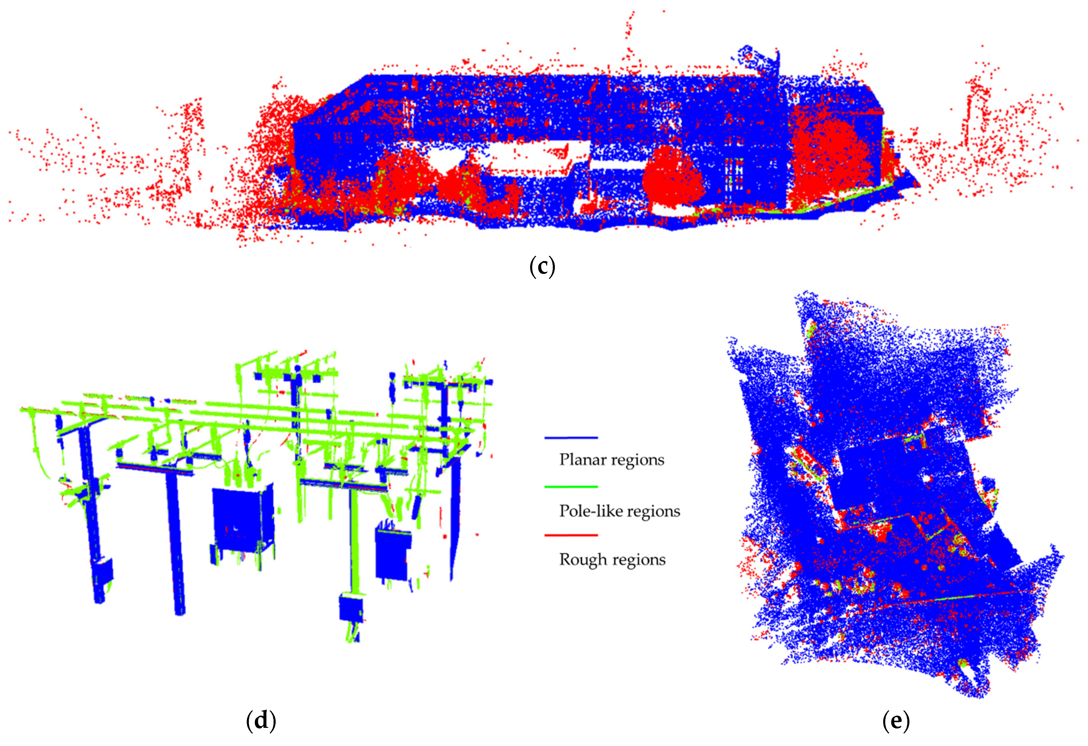
  • Planar and varying-radii pole-like features are simultaneously segmented,
  • ALS, TLS, MTLS, and image-based point clouds can be manipulated by the proposed segmentation procedure,
  • The region-growing process starts from optimally-selected seed regions to reduce the sensitivity of the segmentation outcome to the choice of the seed location,
  • The region-growing process considers variations in the local characteristics of the point cloud (i.e., local point density/spacing and noise level),
  • The QC process considers possible competition among neighboring planar and pole-like features for the same points,
  • The QC procedure considers possible artifacts arising from the sequence of the region growing process, and
  • The QC process considers the possibility of having partially or fully misclassified planar and pole-like features.
The paper starts with a presentation of the proposed segmentation and quality control procedures. Then, comprehensive results from ALS, TLS, and image-based point clouds are discussed to illustrate the feasibility of the proposed procedure. Finally, the paper concludes with a summary of the main characteristics, as well as the limitations of the proposed methodology/framework together with recommendations for future research.

2. Proposed Methodology

As can be seen in Figure 1, the proposed methodology proceeds according to the following steps: (1) structuring and characterization of the point cloud; (2) distance-based region growing starting from randomly-selected seed points to define seed regions with pre-defined size; (3) PCA-based classification and feature modeling of generated seed regions; (4) Sequential region-growing according to the quality of fit between neighboring points and the fitted-model through the constituents of the seed regions; (5) PCA-based classification, model-fitting, and region growing of non-segmented points; (6) distance-based region growing for the segmentation of rough points; and (7) quality control of the segmentation outcome. The following subsections introduce the technical details of these steps.
Figure 1. Framework for the multi-class segmentation and quality control procedure.
Remotesensing 08 00104 g001

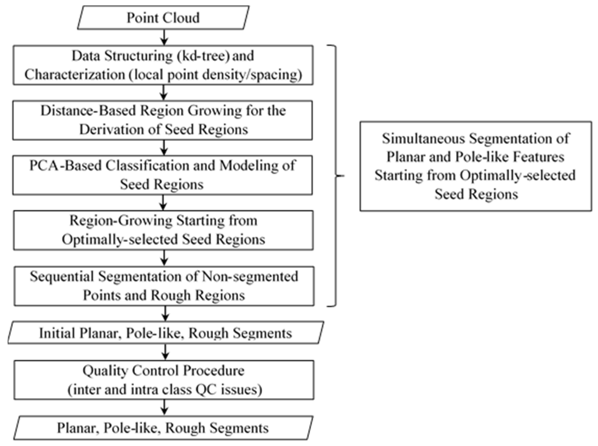
2.1. Simultaneous Segmentation of Planar and Pole-Like Features Starting from Optimally-Selected Seed Regions

In this subsection, we introduce the conceptual basis and implementation details for the first four steps of the processing framework in Figure 1 (i.e., data structuring and characterization, establishing seed regions, PCA-based classification and modeling of the seed regions, and sequential region-growing from optimally-selected seed regions).

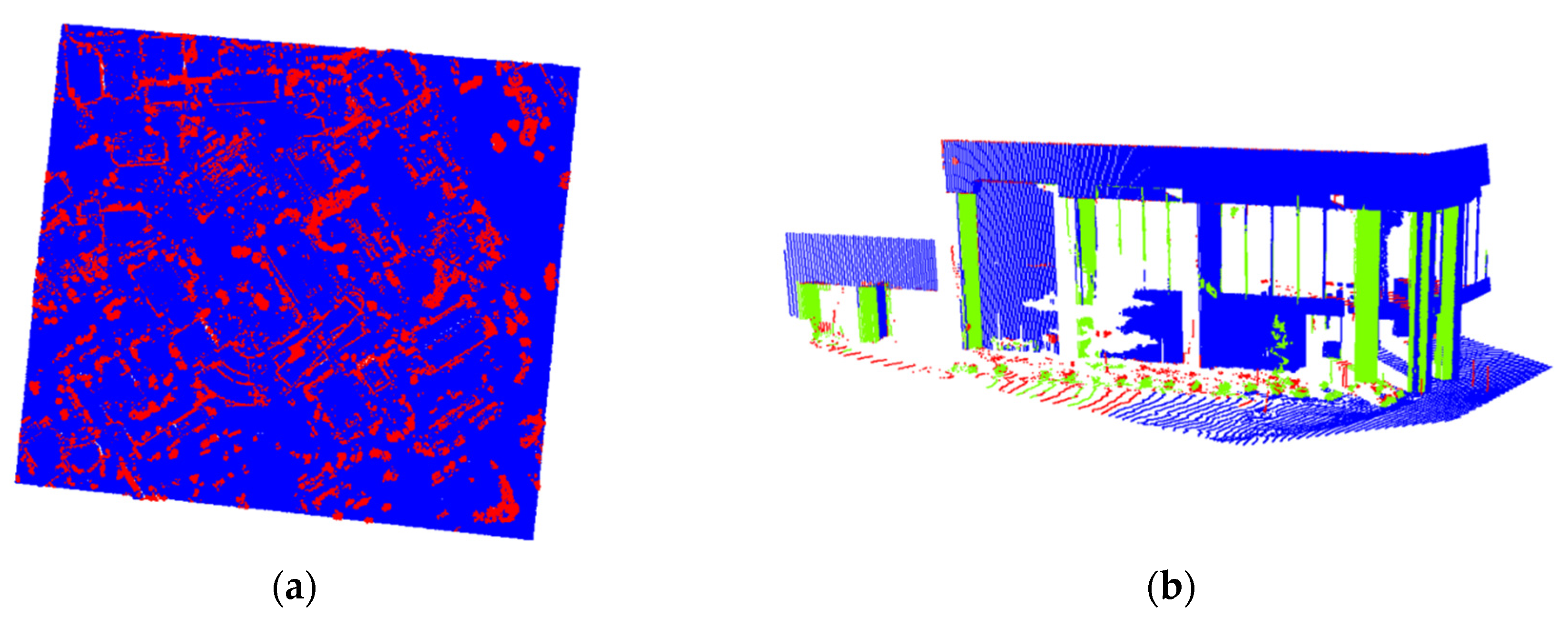
2.1.1. Data Structuring and Characterization

For non-organized point clouds, it is important to re-organize such data to facilitate the identification of the nearest neighbor or nearest n -neighbors for a given point. TIN, grid, voxel, Octree, and kd-tree data structures are possible alternatives for facilitating the search within a non-organized point cloud [39,40,41,42,43,44]. In this research, the kd-tree data structure is utilized for sorting and organizing a set of points since it leads to a balanced tree—i.e., a binary tree with the minimum depth—which improves the efficiency of the neighborhood-search process. The kd-tree data structure is established by recursive sequential subdivision of the three-dimensional space along the X, Y, and Z directions starting with the one that has the longest extent. The splitting plane is defined to be perpendicular to the direction in question and passes through the point with the median coordinate along that direction. The 3D recursive splitting proceeds until all the points are inserted in the kd-tree.
The outcome of any region-growing segmentation approach depends on the search radius, which is used to identify neighboring points that satisfy a predefined similarity criterion. This search radius should be based on the Local Point Density/Spacing (LPD/LPS) for the point under consideration. For either laser-based or image-based point clouds, the LPD/LPS will change depending on the utilized sensor and/or platform as well as the sensor-to-object distance. For image-based point clouds, the LPD/LPS can be also affected by object texture or illumination conditions. Therefore, we need to estimate a unique LPD/LPS for every point within the dataset in question. More specifically, for every point, we establish a local neighborhood that contains a pre-specified number of points. As stated in Lari and Habib [36], the evaluation of the LPD/LPS requires the identification of the nature of the local surface at the vicinity of the query point (i.e., LPD/LPS evaluation depends on whether the local surface is defined by a planar, thin linear, cylindrical, or rough feature—please, refer to the reported statistics in Table 1). The number of used points to define the local surface should be large enough to ensure that the local surface is correctly identified for valid estimation of the LPD/LPS. In this research, a total of 70 points have been used to define the local neighborhood for a given point. Then, a PCA procedure is used to identify the nature of the defined local neighborhood—i.e., determine whether it is part of a planar, pole-like, or rough region [45]. Depending on the identified class, the corresponding LPD— p n t s / m for thin pole-like features, p n t s / m 2 for planar and cylindrical features, and p n t s / m 3 for rough regions—and the corresponding LPS are estimated according to the established measures in Lari and Habib [38].
Table 1. LPD statistics for the different datasets.
ALSTLS1TLS2TLS3DIM
Number of Points812,980170,296201,846455,167230,434
Max. Planar LPD (pts/m2)4.5181549324.5473,443404
Min. Planar LPD (pts/m2)0.0581.687≈0.00017.3511.234
Mean Planar LPD (pts/m2)2.59678127.30517,685104
Max. Linear LPD (pts/m)10.1971408.4731,1860
Min. Linear LPD (pts/m)7.70816.7778.47355.0930
Mean Linear LPD (pts/m)8.96062.3968.4732760
Max. Cylindrical LPD (pts/m2)3.2042,42399934,337375
Min. Cylindrical LPD (pts/m2)2.0596.1321.70710.0633.066
Mean Cylindrical LPD (pts/m2)2.99031341.2166,05546.045
Max. Rough LPD (pts/m3)1.3299,2672,1201,954,8071217
Min. Rough LPD (pts/m3)0.0011.980≈0.00011.6880.053
Mean Rough LPD (pts/m3)0.363181826.238230,796145

2.1.2. Distance-Based Region Growing for the Derivation of Seed Regions

This step starts by forming a set of seed points that are randomly distributed within the point cloud in question. Rather than directly defining seed regions, which are centered at the randomly-established seed points, we define the seed regions through a distance-based region growing. More specifically, starting from a user-defined percentage of randomly-selected seed points, we perform a distance-based region growing (i.e., the spatial closeness of the points to the seed point in question as determined by the LPS is the only used criterion). The distance-based region growing continues until pre-specified region size is attained. This approach for seed-region definition will ensure that the seed region is large enough, while avoiding the risk of having the seed region comprised of points from two or more different classes. Therefore, when dealing with different features that are spatially close to each other, we ensure that the seed regions belong to the individual objects as long as the spatial separation between those features is larger than the LPS. Having larger seed regions that belong to individual objects will lead to better identification of the respective models associated with those neighborhoods, which in turn will increase the reliability of the segmentation procedure.

2.1.3. PCA-Based Classification and Modeling of Seed Regions

Now that we defined the seed regions, we use PCA to identify whether they belong to planar, pole-like, or rough neighborhoods. More specifically, the relationships among the normalized Eigen values of the dispersion matrix of the points within a seed region relative to its centroid are used to identify planar seed regions (i.e., where two of the normalized Eigen values are significantly larger than the third one), pole-like seed regions (i.e., where one of the normalized Eigen values is significantly larger the other two), and rough seed regions (i.e., where the three normalized Eigen values are of similar magnitude). For planar and pole-like seed regions, a Least Squares Adjustment (LSA) model-fitting procedure is used to derive the plane/pole-like parameters together with the quality of fit between the points within the seed region and the defined model as represented by the respective a-posteriori variance factor (this a-posteriori variance factor will be used as an indication of the local noise level within the seed region). For a planar seed region, the LSA estimates the three plane parameters—a, b, and c—using either Equation (1), (2), or (3) (the choice of the appropriate plane equation depends on the orientation of the Eigen vector corresponding to the smallest Eigen value—i.e., the one defining the normal to the plane)—refer to Figure 2. For a pole-like feature, the LSA estimates its radius together with four parameters that define the coordinates of a point along the axis and the axis orientation—p, q, a, and b—using either Equation (4), (5), or (6) (the choice of the appropriate equation depends on the orientation of the Eigen vector corresponding to the largest Eigen value—i.e., the one defining the axis orientation of the pole-like feature)—refer to Figure 3. One should note that the variable t in Equations (4)–(6), depends on the distance between the projection of any point onto the axis of the pole-like feature and the utilized point along the axis—i.e., (p,q,0) for the axis defined by Equation (4), (p,0,q) for the axis defined by Equation (5), or (0,p,q) for the axis defined by Equation (6) (refer to Figure 3).
z = a x + b y + c
y = a x + b z + c
x = a y + b z + c
x = p + t   a y = q + t   b z = t
x = p + t   a y = t z = q + t   b
x = t y = p + t   a z = q + t   b
Figure 2. Representation scheme for 3D planar features; planes that are almost parallel to the x y p l a n e (a); planes that are almost parallel to the x z p l a n e (b); and planes that are almost parallel to the y z p l a n e (c).
Remotesensing 08 00104 g002
Figure 3. Representation scheme for 3D pole-like features; pole-like features that are almost parallel to the z a x i s (a); pole-like features that are almost parallel to the y a x i s (b); and pole-like features that are almost parallel to the x a x i s (c).
Remotesensing 08 00104 g003

2.1.4. Region-Growing Starting from Optimally-Selected Seed Regions

In this research, the seed regions representing planar and pole-like features are sorted according to an ascending order for the evaluated a-posteriori variance factor in the previous step. One should note that such a-posteriori variance factor is an indication of the normal distances between the points within the seed region and the best-fitted model—i.e., it is an indication of the noise level in the dataset as well as the compatibility of the physical surface and the underlying mathematical model. Starting with the seed region that has the minimum a-posteriori variance factor, a region-growing process is implemented while considering the spatial proximity as defined by the LPS and the normal distance to the defined model through the seed region as the similarity criteria. Throughout the region-growing process, the model parameters and a-posteriori variance factor are sequentially updated. For a given seed region, the growing process will proceed until no more points could be added. The sequential region growing according to the established quality of fit—i.e., a-posteriori variance factor—will ensure that seed regions showing better fit to the planar or pole-like feature model are considered first. Thus, rather than starting the region growing from randomly established seed points, we start the growing from locations that exhibit good fit with the pre-defined models for planar and pole-like features.

2.1.5. Sequential Segmentation of Non-Segmented Points and Rough Regions

Depending on the user-defined percentage of seed points, one should expect that some points might not be segmented or considered since they are not within the immediate vicinity of seed points that belong to the same class or they happen to be at the neighborhood of rough seed regions. To consider such situations, we implement a sequential region-growing process by going through the points within the kd-tree data structure starting from its root and identifying the points that have not been segmented/classified so far. Whenever a non-segmented/non-classified point within the kd-tree data structure is encountered, the following region-growing procedure is implemented:
  • Starting from a non-segmented/non-classified point, a distance-based region growing is implemented, according the established LPS, until a pre-defined seed-region size is achieved.
  • For the established seed region, PCA is used to decide whether the seed region represents planar, pole-like, or rough neighborhood. If the seed region is deemed as being part of a planar or pole-like feature, the parameters of the respective model are estimated through a LSA procedure.
  • A region-growing process is carried out using the LPS and quality of fit with the established model in the previous step as the similarity measures. Throughout the region-growing process, the model parameters and the respective a-posteriori variance factor are sequentially updated.
  • Steps 1–3 are repeated until all the non-segmented/non-classified nodes within the kd-tree data structure are considered.
The last step of the segmentation process, is grouping neighboring points that belong to rough regions. This is carried out according to the following steps:
  • For the seed regions, which have been classified as being part of rough neighborhoods during the first or the second stages of the segmentation procedure, we conduct a distance-based region-growing of non-segmented points.
  • Finally, we inspect the kd-tree starting from its root node to identify non-segmented/non-classified nodes, which are utilized as seed points for a distance-based segmentation of rough regions.
At this stage, the constituents of a point cloud have been classified and segmented into planar, pole-like, and rough segments. For planar and pole-like features, we have also established the respective model parameters and a-posteriori variance factor, which describes the average normal distance between the constituents of a region and the best-fit model.

2.2. Quality Control of the Segmentation Outcome

In spite of the facts that, (1) the proposed region-growing segmentation strategy has been designed to optimally-select seed regions that exhibit the best quality of fit to the LSA-based planar/pole-like models; and (2) the region growing is based on the established LPS for the individual points, one cannot guarantee that the segmentation outcome will be perfect (i.e., the segmentation outcome might still exhibit artifacts). For example, one should expect that segmented regions at an earlier stage might invade segmented regions at a later stage. Additionally, due to the location of the randomly-established seed points and the nature of the objects within the point cloud, there might be instances where seed regions are wrongly classified (e.g., a portion of a planar feature is wrongly classified as a pole-like feature or a set of contiguous pole-like features are identified as a planar segment). As has been mentioned in the Introduction, prior research has dealt with the detection and mitigation of over-segmentation and under-segmentation problems. However, prior research does not consider potential artifacts that might arise when simultaneously segmenting planar, pole-like, and rough regions. The proposed quality control framework proceeds according to the following three stages; namely, (1) developing a list of hypothesized artifacts/problems that might take place during the segmentation process; (2) developing procedures for the detection of instances of such artifacts/problems without the need for having reference data; and (3) developing approaches to mitigate such problems whenever detected. The following list provides a summary of hypothesized problems that might take place within a multi-class simultaneous segmentation of planar and pole-like features; Figure 4a–f is a schematic illustration of such problems—in sub-figures a ,   b ,   c ,   e ,   and   f classified planar regions are displayed in light blue while classified pole-like features are displayed in light green:
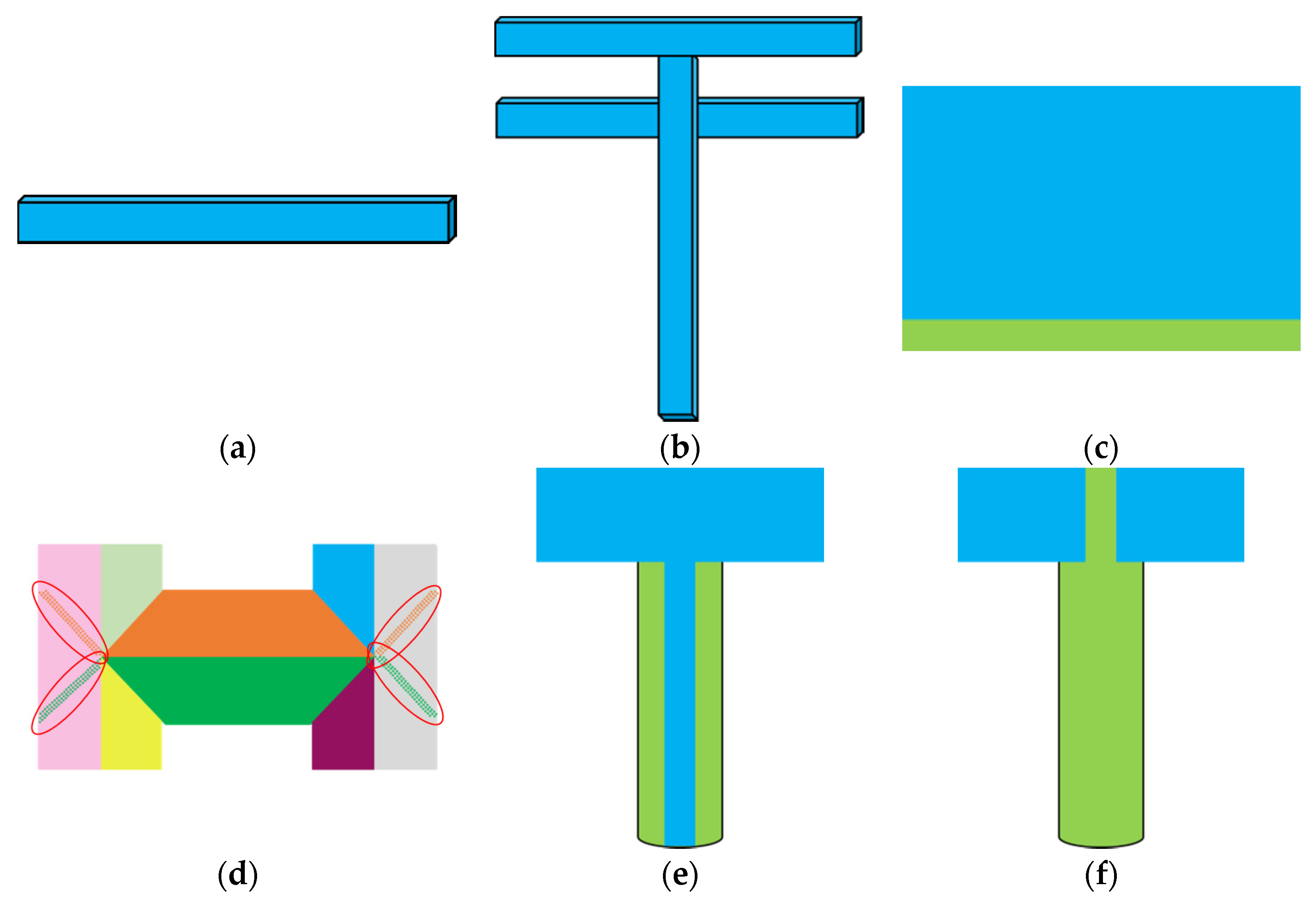
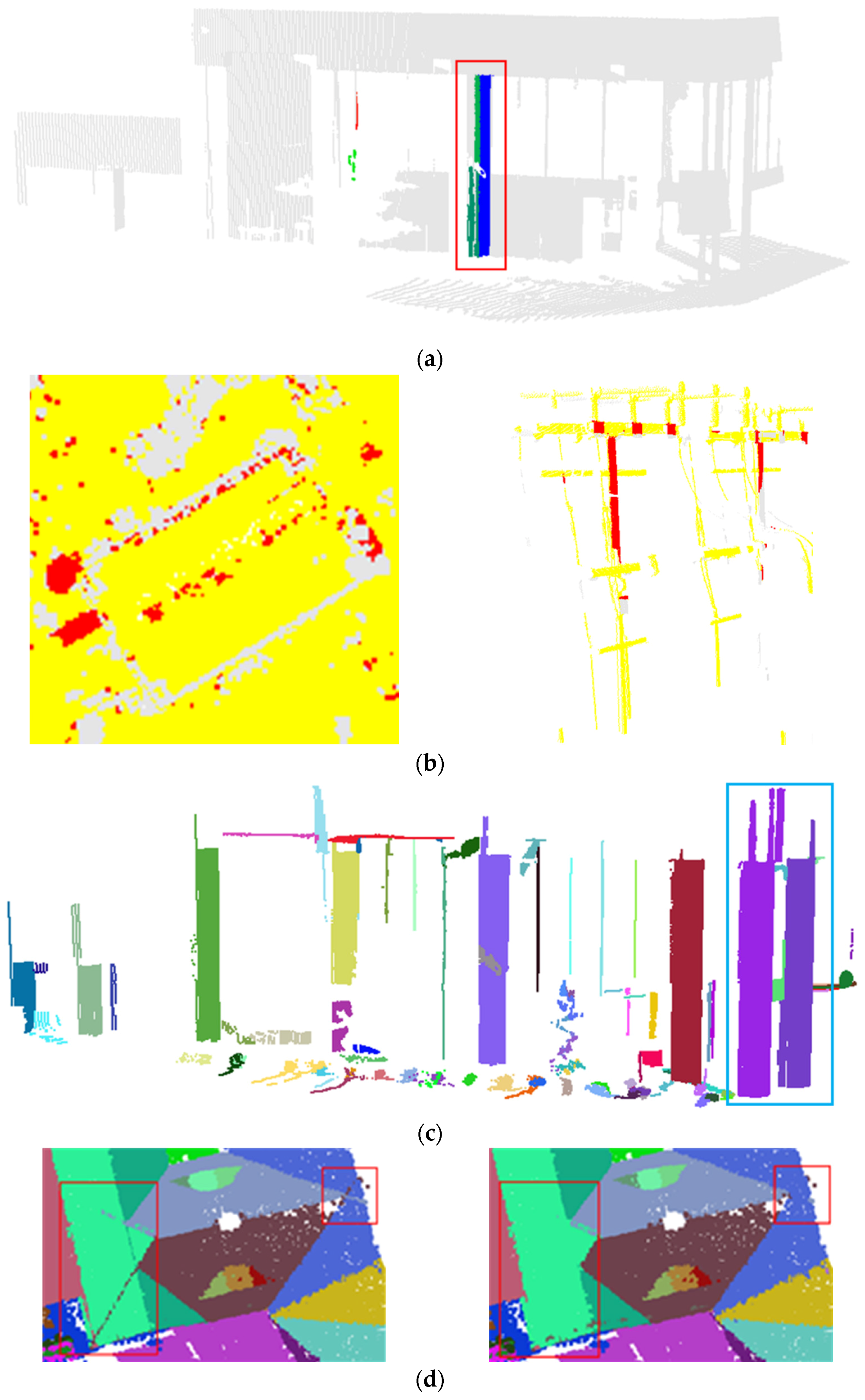
  • Misclassified planar features: Depending on the LPD/LPS and pre-set size for the seed regions, a pole-like feature might be wrongly classified as a planar region. This situation might be manifested in one of the following scenarios:
    • Single pole-like feature is wrongly classified as a planar region (Figure 4a), and
    • Multiple contiguous pole-like features are classified as a single planar region (Figure 4b).
  • Misclassified linear features: depending on the location of the randomly-established seed points, a portion of a planar region might be classified as a single pole-like feature (Figure 4c).
  • Partially misclassified planar and pole-like features: Depending on the order of the region growing process, segmented planar/pole-like features at the earlier stage of the segmentation process might invade neighboring planar/pole-like features. This situation might be manifested in one of the following scenarios:
    • Earlier-segmented planar regions invade neighboring planar features (Figure 4d),
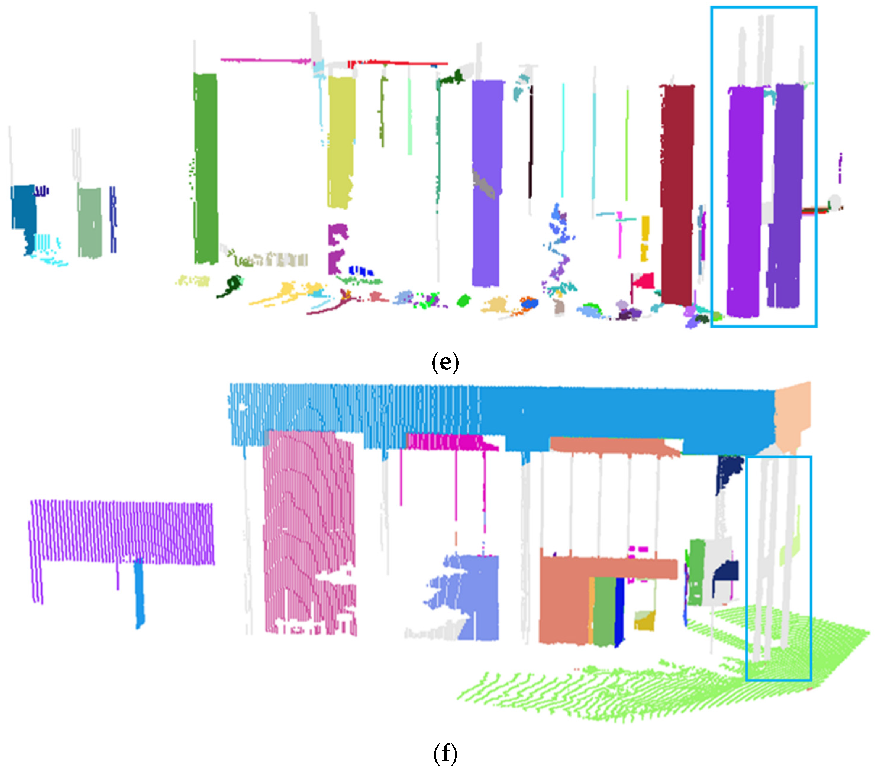
    • Earlier-segmented planar regions fully or partially invade neighboring pole-like features (Figure 4e, where a planar region partially invade a neighboring pole-like feature), and
    • Earlier-segmented pole-like features invade neighboring planar features (Figure 4f).
Figure 4. Possible segmentation artifacts; misclassified planar features (a,b); misclassified pole-like feature (c); partially misclassified planar features (d,e); and partially misclassified pole-like feature (f)—planar and pole-like features are displayed in light blue and light green, respectively, in subfigures (a), (b), (c), (e), (f).
Remotesensing 08 00104 g004
The above problems can be categorized as follows: (1) Interclass competition for neighboring points; (2) Intraclass competition for neighboring points; and (3) Fully/partially-misclassified planar and pole-like features. To deal with such segmentation problems, we introduce the following procedure to detect and mitigate instances of such problems:
  • itial mitigation of interclass competition for neighboring points: A key problem in region-growing segmentation is that derived regions at an early stage might invade neighboring features of the same or different class, which are derived at a later stage. In this QC category, we consider potential invasion among features that belong to different classes. Specifically, for segmented features in a given class (i.e., planar or pole-like features), features in the other classes (including rough regions) will be considered as potential candidates that could be incorporated into the constituent regions of the former class. For example, the constituents of pole-like features and rough regions will be considered as potential candidates that could be incorporated into planar features. In this case, if a planar feature has potential candidates, which are spatially close as indicated by the established LPS, and the normal distance between those potential candidates and the LSA-based model through that planar feature is within the respective a-posteriori variance factor, those potential candidates will be incorporated into the planar feature in question. The same procedure is applied for pole-like features, while considering planar and rough regions as potential candidates. In this regard, the respective QC measure— Q C i n t e r c l a s s   c o m p e t i t i o n —is evaluated according to Equation (7), where n i n c o r p o r a t e d represents the number of incorporated points from other classes and n p o t e n t i a l   c a n d i d a t e s represents the number of potential candidates for this class. For that QC measure, lower percentage indicates lower instances of points that have been incorporated from other classes.
    Q C i n t e r c l a s s   c o m p e t i t i o n =   n i n c o r p o r a t e d n p o t e n t i a l   c a n d i d a t e s  
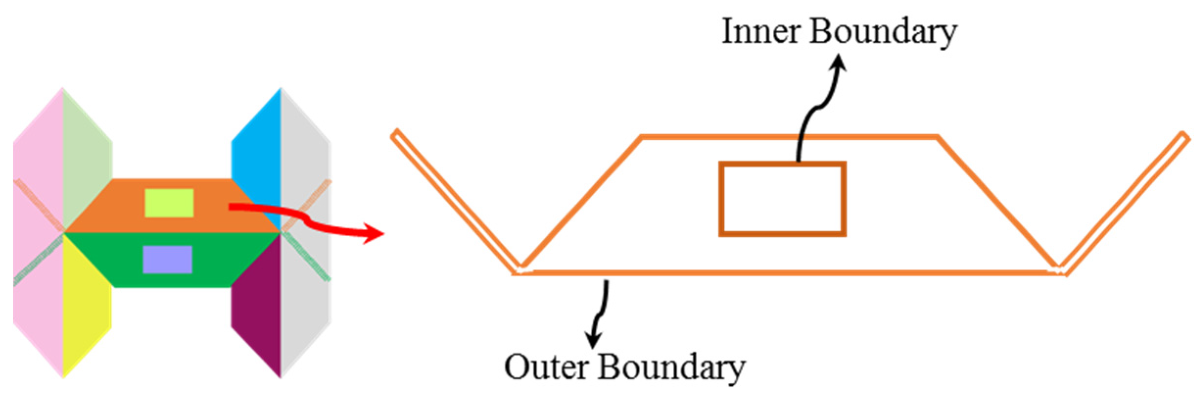
  • Mitigation of intraclass competition for neighboring points: This problem takes place whenever a feature, which has been derived at the earlier stage of the region growing, invades other features from the same class that have been segmented at a later stage. One can argue that intraclass competition for pole-like features is quite limited (this is mainly due to the narrow spread of pole-like features across its axis). Therefore, for this QC measure, we only consider intraclass completion for planar features (as can be seen in Figure 4d, where the middle planar regions invade the left and right planar features with the invading portions highlighted by red ellipses). Detection and mitigation of such problem starts by deriving the inner and outer boundaries of the segmented planar regions (Figure 5 illustrates an example of inner and outer boundaries for a given segment). The inner and outer boundaries can be derived using the minimum convex hull and inter-point-maximum-angle procedures presented by Sampath and Shan [44] and Lari and Habib [45], respectively. Then, for each of the planar regions, we check if some of their constituents are located within the boundaries of neighboring regions and at the same time the normal distances between such constituents and the fitted model through the neighboring regions are within their respective a-posteriori variance factor. In such a case, the individual points that satisfy these conditions are transformed from the invading planar feature to the invaded one. For such QC category, the respective measure is determined according to Equation (8), where n i n v a d i n g represents the number of invading planar points that have been transformed from the invading to the invaded segments and n p l a n e   t o t a l represents the total number of originally-segmented planar points. In this case, lower percentage indicates lower instances of such problem.
    Q C i n t r a c l a s s   c o m p e t i t i o n =   n i n v a d i n g n p l a n e   t o t a l  
    Figure 5. Inner and outer boundary derivation for the identification of intraclass competition for neighboring points.
    Figure 5. Inner and outer boundary derivation for the identification of intraclass competition for neighboring points.
    Remotesensing 08 00104 g005
  • Single pole-like feature wrongly classified as a planar one: To detect such instances (Figure 4a is a schematic illustration of such situation), we perform PCA of the constituents of the individual planar features. For such segmentation problem, the PCA-based normalized Eigen values will indicate 1-D spread of such regions. Whenever such scenario is encountered, the LSA-based parameters of the fitted cylinder through this feature together with the respective a-posteriori variance factor are derived. The planar feature will be reclassified as a pole-like one if the latter’s a-posteriori variance factor is almost equivalent to the planar-based one. For this case, the respective QC measure— Q C r e c l a s s i f i e d   l i n e a r   f e a u r e —is represented by Equation (9), where n r e c l a s s i f i e d   l i n e s is the number of points within reclassified linear features and n p l a n e   t o t a l is the total number of points within the originally-segmented planar features. In this case, lower percentage indicates fewer instances of such a problem.
    Q C r e c l a s s i f i e d   l i n e a r   f e a t u r e s =   n r e c l a s s i f i e d   l i n e s n p l a n e   t o t a l  
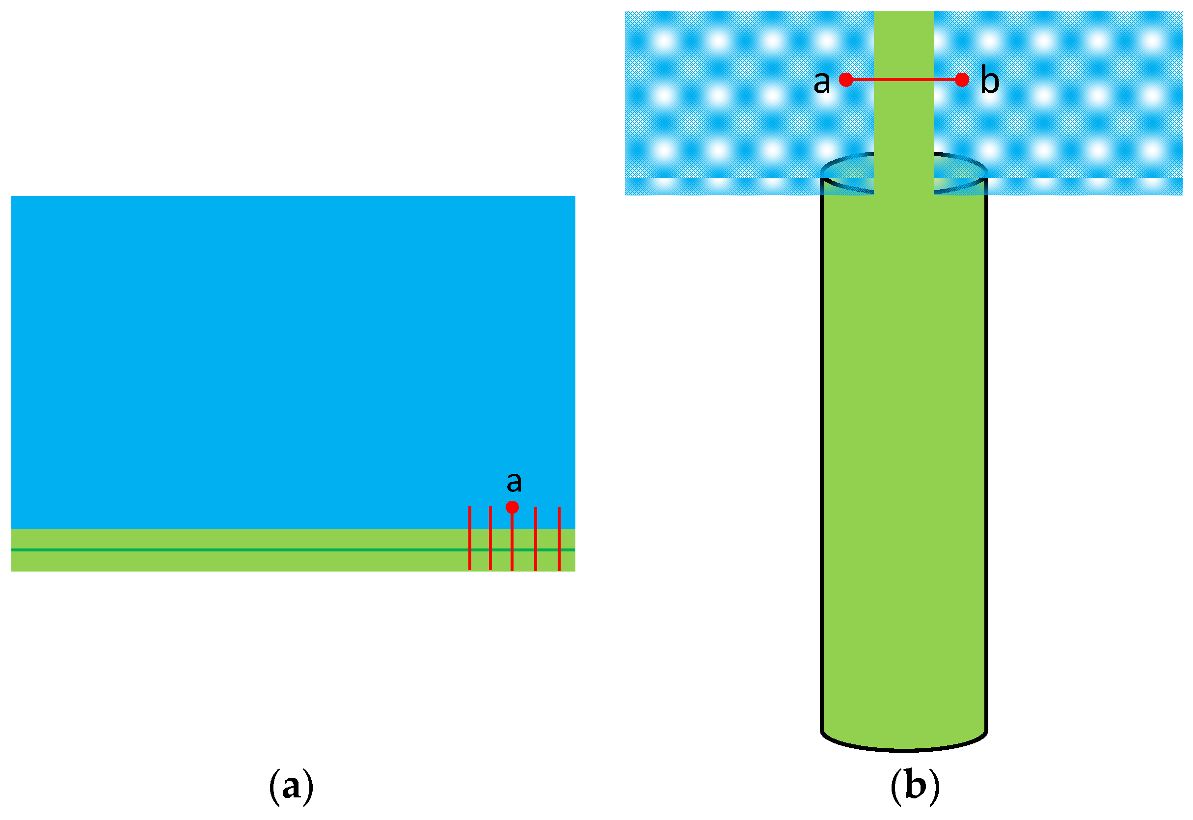
  • Mitigation of fully or partially misclassified pole-like features: For this problem (as illustrated by Figure 4c,f), we identify pole-like features or portions of pole-like features that are encompassed within neighboring planar features. The process starts with identifying neighboring pole-like and planar features where the axis of the pole-like feature is perpendicular to the planar-feature normal. Then, the constituents of the pole-like feature are projected onto the plane defined by the planar feature. Instances, where the pole-like feature is encompassed—either fully or partially—within the planar feature, are identified by slicing the pole-like feature in the across direction to its axis. For each of the slices, we determine the closest planar point(s) that does (do) not belong to the pole-like feature in question (e.g., point a in Figure 6a or points a   a n d   b in Figure 6b). If the closest point(s) happen to be immediate neighbor(s) of the constituents of that slice (as defined by the established LPS), then one can suspect that the portion of the pole-like feature at the vicinity of that slice might be encompassed within the neighboring planar region (i.e., that portion of the pole-like feature might be invading the planar region). To confirm or reject this suspicion, we evaluate the normal distances between the constituents of the slice and the neighboring planar region. If these normal distances are within the respective a-posteriori variance factor for the planar region, we confirm that the slice is encompassed within the planar region. Whenever the pole-like feature is fully encompassed within the planar region (Figure 6a), all the slices will have immediate neighbors from that planar region while having minimal normal distances. Consequently, the entire pole-like feature will be reassigned to the planar region. On the other hand, whenever the linear feature is partially encompassed within the planar region, we identify the slices where the closest neighbors to such slices are not immediate neighbors (Figure 6b). The portion of the pole-like feature, which is defined by such slices, will be retained while the other portion will be reassigned to the planar region. The QC measure in this case is defined by Equation (10), where n e n c o m p a s s e d   l i n e   p o i n t s   represents the number of points within the pole-like feature that are encompassed within the planar feature and n l i n e   t o t a l is the total number of points within the originally-segmented linear features. Lower percentage indicates fewer instances of such problem.
    Q C p a r t i a l l y / f u l l y   m i s c l a s s i f i e d   p o l e l i k e   f e a t u r e s =   n e n c o m p a s s e d   l i n e   p o i n t s n l i n e   t o t a l  
    Figure 6. Slicing and immediate-neighbors concept for the identification of fully/partially misclassified pole-like features (a)/(b).
    Figure 6. Slicing and immediate-neighbors concept for the identification of fully/partially misclassified pole-like features (a)/(b).
    Remotesensing 08 00104 g006
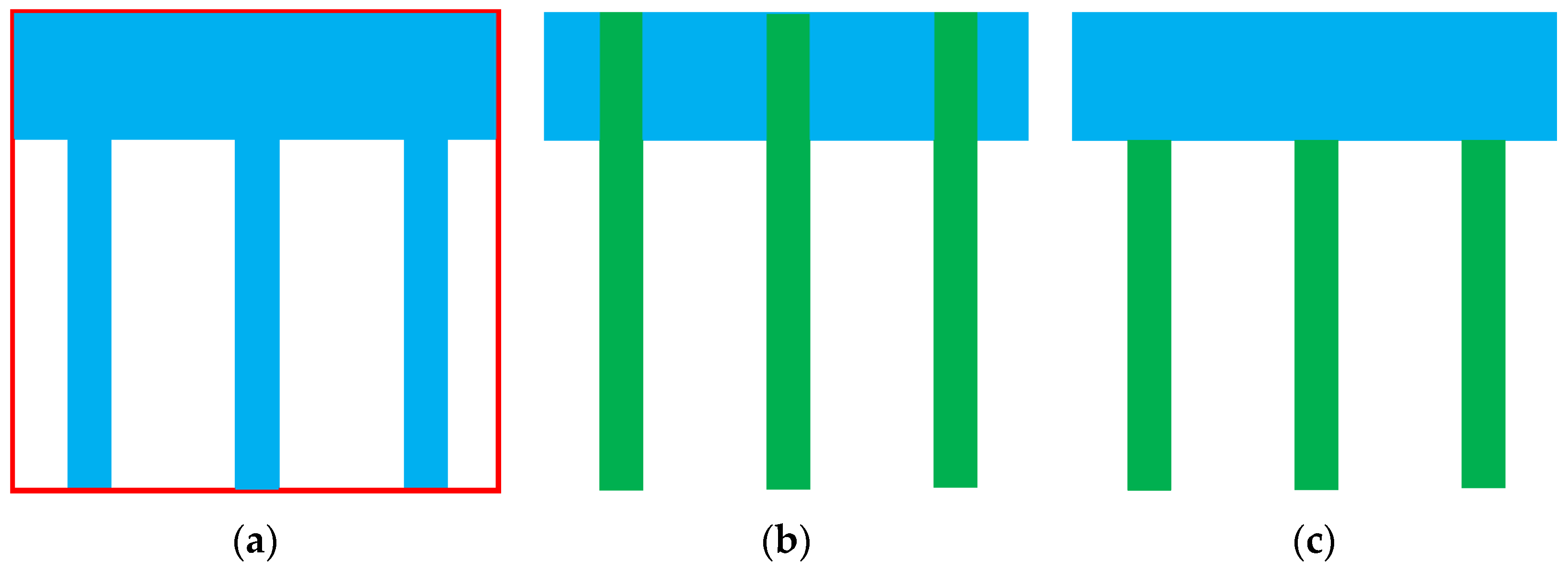
  • Mitigation of fully or partially misclassified planar features: The conceptual basis of the implemented procedure to detect instances of such problem (as illustrated by Figure 4b,e) is that whenever planar features are either fully (Figure 4b) or partially (Figure 4e) misclassified, a significant portion of the encompassing Minimum Bounding Rectangle (MBR) will not be occupied by those features (refer to Figure 7a). In this regard, one should note that the MBR denotes the smallest area rectangle that encompasses the identified boundary of the planar region in question [46]. Therefore, to detect instances of such problem, we start by defining the MBR for the individual planar regions. Then, we evaluate the ration between the area of the planar region in question and the area of the encompassing MBR. Whenever this area is below a pre-defined threshold, we suspect that the planar feature in question might contain pole-like features, which will take the form of tentacles to the original planar region (as can be seen in Figure 7a). To identify such features, we perform a 2D-linear feature segmentation procedure, which is similar to the one proposed earlier with the exception that it is conducted in 2D rather than 3D (i.e., the line parameters would include slope, intercept, and width)—refer to Figure 7b. More specifically, pre-defined percentage of seed points are established. Then, a distance-based region growing is carried out to define seed regions with pre-set size. A 2D-PCA and line fitting procedure is conducted to identify seed regions that represent 2D lines. Those seed regions are then incorporated within a region-growing process that considers both the spatial closeness of the points and their normal distance to the fitted 2D lines. Following the 2D-line segmentation, an over-segmentation quality control is carried out to identify single linear features that have been identified as multiple ones. Moreover, the conducted QC in the previous step is implemented to identify partially misclassified linear features—i.e., the invading portion of the linear feature(s) (refer to Figure 7c). The QC measure for such problem is evaluated according to Equation (11), where n m i s c l a s s i f i e d   p l a n e   p o i n t s represents the number of points within the planar feature that belong to 2D lines and n p l a n e   t o t a l is the total number of originally-segmented planar points. Lower percentage indicates fewer instances of such problem.
    Q C p a r t i a l l y / f u l l y   m i s c l a s s i f i e d   p l a n a r   f e a t u r e s =   n m i s c l a s s i f i e d   p l a n e   p o i n t s n p l a n e   t o t a l  
Figure 7. Segmented planar feature—in light blue—and the encompassing MBR—in red (a); segmented linear features—in green (b); and final segmentation after the identification of partially-misclassified linear features (c).
Remotesensing 08 00104 g007

3. Experimental Results

To illustrate the performance of the segmentation and quality control procedure, this section provides the segmentation and quality control results using ALS, TLS, and image-based point clouds. The main objectives of the conducted experiments are as follows:
  • Prove the feasibility of the proposed segmentation procedure in handling data with significant variation in LPD/LPS as well as inherent noise level,
  • Prove the feasibility of the proposed segmentation procedure in handling data with different distribution and concentration of planar, pole-like, and rough regions,
  • Prove the capability of the proposed QC procedure in detecting and quantifying instances of the hypothesized segmentation problems, and
  • Prove the capability of the proposed QC procedure in mitigating instances of the hypothesized segmentation problems.
The following subsections provide the datasets description, segmentation results, and the outcome of the quality control procedure.

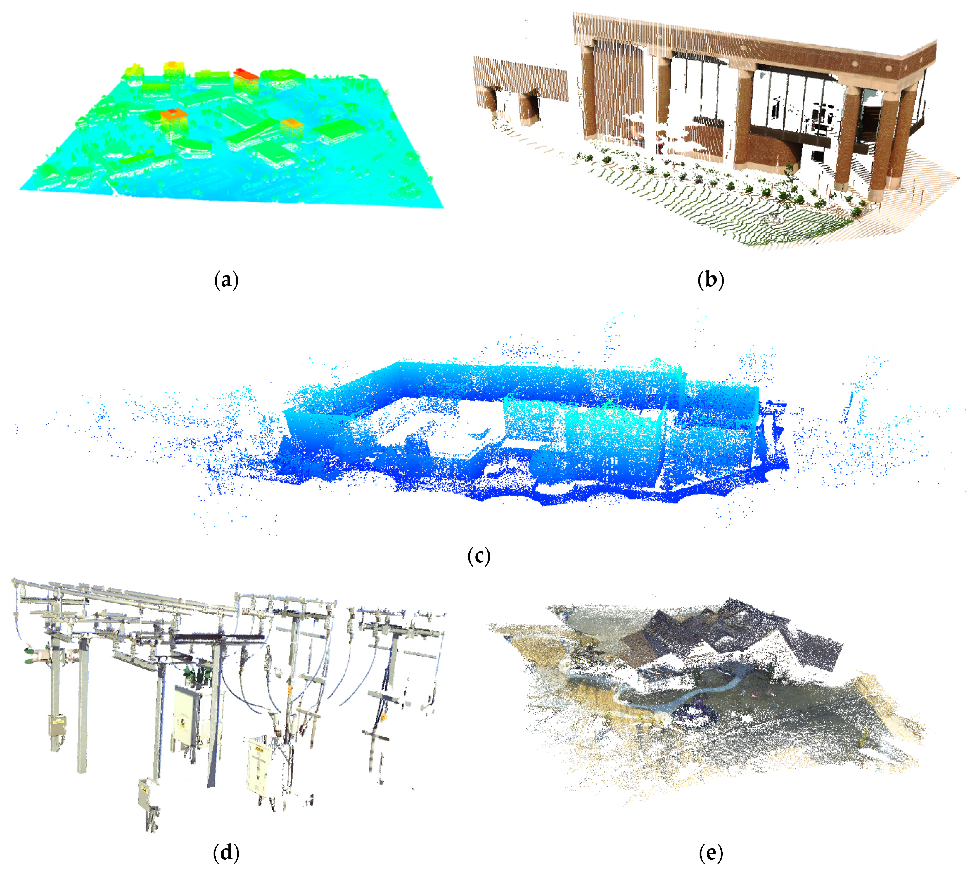
3.1. Datasets Description

Airborne Laser Scanner Dataset—ALS: This dataset is captured by an Optech ALTM 3100 over an urban area that includes planar roofs, roads, and trees/bushes. The extent of the covered area is roughly 0.5 km × 0.5 km. Figure 8a shows a perspective view of the ALS point cloud, where the color is based on the height of the different points.
First Terrestrial Laser Scanner Dataset—TLS1: This dataset is captured by a FARO Focus3D X330 scanner. The effective scan distance for this scanner ranges from 0.6 m up to 330 m. The ranging error is ±2 mm. The scanner is positioned at the vicinity of a building façade with planar and cylindrical features whose radii is almost 0.6 m. The extent of the covered area is approximately 35 m × 20 m × 10 m. Figure 8b illustrates the perspective view of this dataset with the colors derived from the scanner-mounted camera.
Second Terrestrial Laser Scanner Dataset—TLS2: This dataset is captured by Leica HDS 3000 scanner. The effective san distance for this unit ranges up to 300 m with ±6 mm position accuracy at 50 m. The covered area includes a planar building façade, some light poles, and trees/bushes. The extent of the covered area is almost 250 m × 200 m × 26 m. A perspective view of this dataset is illustrated in Figure 8c.
Third Terrestrial Laser Scanner Dataset—TLS3: This dataset covers an electrical substation and is captured by a FARO Focus3D X130 scanner. The effective scan distance ranges from 0.6 m up to 130 m. The ranging error is ±2 mm. The dataset is mainly comprised of pole-like features with relatively small radii. The extent of the covered area is roughly 12 m × 10 m × 6 m. A perspective view of this dataset is provided in Figure 8d with the colors derived from the scanner-mounted camera.
Dense Image Matching Dataset—DIM: This dataset, which is shown in Figure 8e, is derived from a block of 28 images captured by a GoPro 3 camera onboard a DJI Phantom 2 UAV platform over a building with complex roof structure. The extent of the covered area is approximately 100 m × 130 m × 17 m. A Structure from Motion (SfM) approach developed by He and Habib [46] is adopted for automated determination of the frame camera EOPs as well as sparse point cloud representing the imaged area relative to an arbitrarily-defined local reference frame. Then, a semi-global dense matching is used to derive a dense point cloud from the involved images [9].
The processing framework starts with data structuring as well as deriving the LPD/LPS for the point clouds in the different datasets. For LPD/LPS estimation, the closest 70 points have been used. Ratios among the PCA-based Eigen values are used to classify the local neighborhoods into planar, pole-like, and rough regions. For Planar regions, the smallest normalized Eigen value should be less than 0.03, while the ration between the other two should be larger than 0.6. For pole-like neighborhoods, on the other hand, the largest normalized Eigen value should be larger than 0.7. The number of the involved points and the statistics of the LPD for the different datasets are listed in Table 1, where one can observe the significant variations in the derived LPD values.
Figure 8. Perspective views of the point clouds from the ALS (a); TLS1 (b); TLS2 (c); TLS3 (d); and DIM (e) datasets.
Remotesensing 08 00104 g008

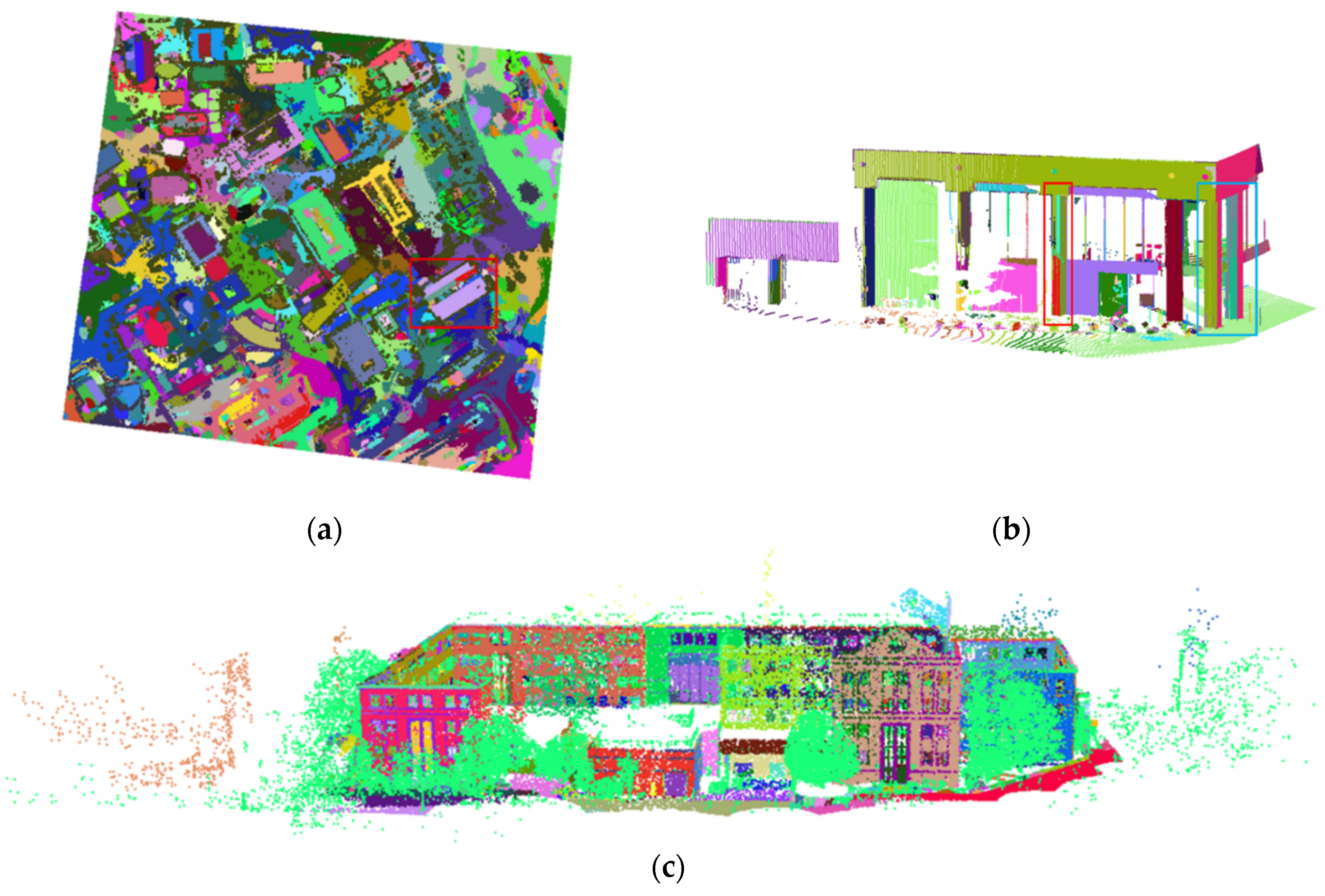
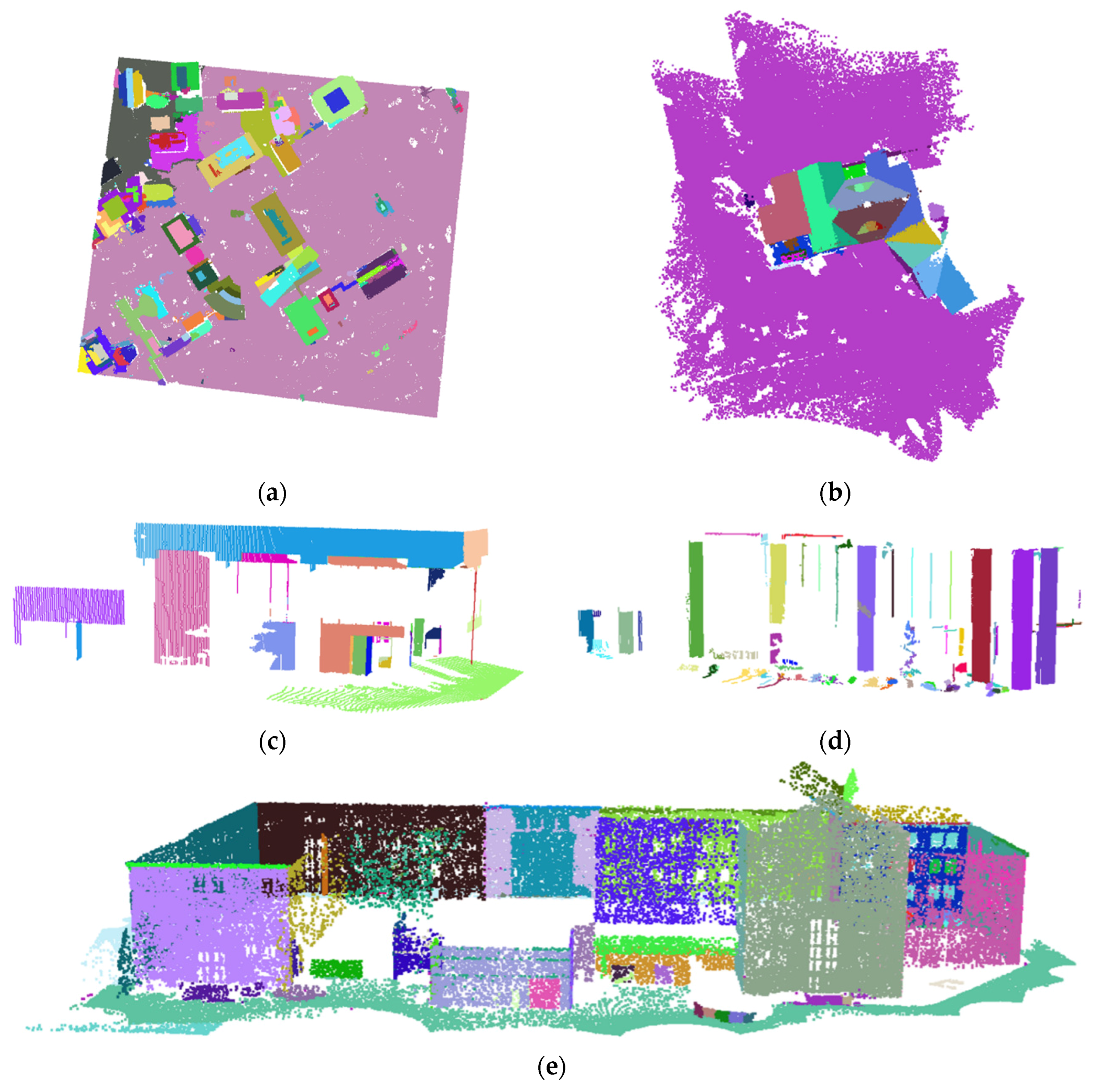
3.2. Segmentation Results

This section provides the segmentation results for planar, pole-like, and rough regions from the different datasets. Before discussing the segmentation results, we introduce the different thresholds, the rationale for setting them up, and the utilized numerical values. The proposed region-growing segmentation methodology involves three thresholds: (1) Percentage of randomly-selected seed points relative to the total number of available points within the dataset—For the above datasets, this percentage is set to 10%. One should note that using larger percentage value did not make a significant impact on the segmentation results; (2) Pre-set size of the seed regions—This size should be set-up in a way to ensure that the seed region is large enough for reliable estimation of the model parameters associated with that region. For the conducted tests, the pre-set region size is set to 100; (3) Normal distance threshold—In general, the normal distance threshold for the region-growing process is based on the derived a-posteriori variance factor from the LSA parameter estimation procedure. However, we set upper threshold values that depend on the sensor specifications (i.e., the normal distance thresholds are not allowed to go beyond these values). For the conducted experiments, the ALS-based region-growing normal distance is set to 0.2 m. For the TLS and DIM datasets, the normal distance threshold is set to 0.05 m. The proposed methodology is implemented in C#. The experiments are conducted using a computer with 16 GB RAM and Intel(R) Core(TM) i7-4790 CPU @3.60 GHz. The time performance of the proposed data structuring, characterization, and segmentation is listed in Table 2.
Table 2. Time performance of the proposed segmentation.
ALSTLS1TLS2TLS3DIM
Number of Points812,980170,296201,846455,167230,434
Data Structuring and Characterization (mm:ss)08:1501:4802:0206:5702:34
Segmentation Time (mm:ss)11:4002:5501:3306:3703:56
Total Time (mm:ss)19:5504:4303:3513:3406:30
Figure 9 and Figure 10 present the feature classification and segmentation results, respectively. For the classification results in Figure 9, planar, pole-like, and rough regions are shown in blue, green, and red, respectively. As can be seen in Figure 9, ALS, TLS2, and DIM datasets are mainly comprised of planar and rough regions. TLS1 and TLS3, on the other hand, mainly include planar and pole-like features, where large-radii pole-like features are present in TLS1 and the majority of TLS3 is comprised of small-radii cylinders. In Figure 10, the segmented planar, pole-like, and rough regions are shown in different colors. Visual inspection of the results in Figure 10 indicates that a good segmentation has been achieved. To quantitatively evaluate the quality of such segmentation, the previously-discussed QC measures are used to denote the frequency of detected artifacts.
Figure 9. Perspective views of the classified point clouds for the ALS (a); TLS1 (b); TLS2 (c); TLS3 (d); and DIM (e) datasets (planar, pole-like, and rough regions are shown in blue, green, and red, respectively).
Remotesensing 08 00104 g009aRemotesensing 08 00104 g009b
Figure 10. Perspective views of the segmented point clouds for the ALS (a); TLS1 (b); TLS2 (c); TLS3 (d); and DIM (e) datasets (different segments are shown in different colors).
Remotesensing 08 00104 g010aRemotesensing 08 00104 g010b

3.3. Quality Control Outcome

The quality control procedure has been implemented according to the following sequence: QC1) detection and mitigation of single pole-like features that have been misclassified as planar ones, QC2) initial mitigation of interclass competition for neighboring points, QC3) detection and mitigation of over-segmentation problems, QC4) detection and mitigation of intraclass competition for neighboring points, QC5) detection and mitigation of fully/partially misclassified pole-like features, and finally QC6) detection and mitigation of fully/partially misclassified planar features. One should note that for QC3, the respective over-segmentation measure is evaluated as the ration between the merged segments in a given class relative to the total number of segments in that class. Figure 11, presents the segmentation results following these QC procedures. For TLS1 and TLS3, segmentation results for planar and pole-like features are presented separately since those datasets have significant portions that pertain to such classes. Figure 12 illustrated examples of the detected/mitigated problems through the different QC measures. More specifically, Figure 12a shows portions of a cylindrical column, as highlighted by the red rectangle, that have been originally classified as planar regions and after QC1, they have been correctly reclassified as pole-like features. Figure 12b shows examples of points from other classes, in red, that have been incorporated into planar and pole-like features, in yellow, after implementing QC2. An example of corrected over-segmentation of pole like features after QC3 is illustrated in Figure 12c (compare the segmentation results in Figure 10b and Figure 12c). Detection and mitigation of intraclass competition for neighboring points after QC4 is shown in Figure 12d (refer to the highlighted regions within the red rectangles before and after QC4). The results of mitigating fully/partially misclassified linear regions after QC5 are shown in Figure 12e (refer to the results after the over-segmentation in Figure 12c and those in Figure 12e, where one can see the correct mitigation of partially-misclassified pole-like features). Finally, Figure 12f shows an example of the segmentation results after applying QC6 that identifies/corrects partially/fully misclassified planar features (compare the results in Figure 10b and Figure 12f). The proposed QC procedures provide quantitative measures that indicate the frequency of the segmentation problems. Such quantitative measures are presented in Table 3, where closer investigation reveals the following:
  • For TLS1 and TLS3, which include significant number of pole-like features, a higher percentage of misclassified single pole-like features (QC1) is observed. TLS1 has pole-like features with larger radii. Therefore, there is higher probability that seed regions along cylindrical features with high point density are misclassified as planar ones. For TLS3, misclassified pole-like features are caused by having several thin beams in the dataset.
  • For interclass competition for neighboring points (QC2), airborne datasets with predominance of planar features have higher percentage of Q C i n t e r c l a s s   c o m p e t i t i o n ( p l a n a r ) —refer to the results for the ALS and DIM datasets. On the other hand, Q C i n t e r c l a s s   c o m p e t i t i o n ( p o l e l i k e ) has higher percentages in datasets that have significant portions belonging to cylindrical features (i.e., TLS1 and TLS3).
  • Due to inherent noise in the datasets as well as the strict normal distance thresholds as defined by the derived a-posteriori variance factor, over-segmentation problems (QC4) are present. In this regard, one should note that over-segmentation problems are easier to handle than under-segmentation ones, which could arise from relaxed normal-distance thresholds.
  • Intraclass competition for neighboring points (QC4) are quite minimal. This is evident by the reported low percentages for this category.
  • For partially/misclassified pole-like features, higher percentages of QC5 when dealing with low number of points in such classes is not an indication of a major issue in the segmentation procedure (e.g., QC5 for ALS and DIM where the percentages of the points that belong to pole-like feature are almost 0% and 4%, respectively).
  • For partially/misclassified planar features, higher percentages of QC6 should be expected when dealing with datasets that have pole-like features with large radii or several interconnected linear features that are almost coplanar (this is the case for TLS1 and TLS3, respectively).
Figure 11. Perspective views of the segmented point clouds after the quality control procedure for the ALS–planar (a); DIM–planar (b); TLS1–planar (c); TLS1–pole-like (d); TLS2–planar (e); TLS3–planar (f); and TLS3–pole-like (g) datasets—different segments are shown in different colors.
Remotesensing 08 00104 g011aRemotesensing 08 00104 g011b
Table 3. QC measures for the different datasets.
ALSTLS1TLS2TLS3DIM
Q C 1 n r e c l a s s i f i e d   l i n e s /
n p l a n e   t o t a l /
Q C r e c l a s s i f i e d   l i n e a r   f e a u r e
101/
716,628/
≈0.000
5,439/
123,370/
0.044
402/
126,193/
0.003
25,484/
224,635/
0.113
71/
211,553/
≈0.000
Q C 2 Planar n i n c o r p o r a t e d /
n p o t e n t i a l   c a n d i d a t e s /
Q C i n t e r c l a s s   c o m p e t i t i o n
31,700/
96,453/
0.328
5,457/
52,365/
0.104
2,788/
76,055/
0.036
24,469/
256,016/
0.095
3,991/
18,952/
0.210
Q C 2 Pole-like n i n c o r p o r a t e d /
n p o t e n t i a l   c a n d i d a t e s /
Q C i n t e r c l a s s   c o m p e t i t i o n
0/
812,879/
0
22,193/
123,042/
0.180
4,379/
194,014/
0.022
29,340/
208,937/
0.140
5,198/
227,486/
0.022
Q C 3 Planar n m e r g e d   p l a n a r /
n s e g m e n t e d   p l a n a r /
Q C o v e r   s e g m e n t a t i o n
618/
801/
0.771
23/
59/
0.389
278/
367/
0.757
8/
86/
0.093
163/
195/
0.835
Q C 3 Pole-like n m e r g e d   l i n e a r /
n s e g m e n t e d   l i n e a r /
Q C o v e r   s e g m e n t a t i o n
0/
4/
0
21/
113/
0.185
8/
144/
0.055
152/
430/
0.353
38/
55/
0.69
Q C 4 n i n v a d i n g /
n p l a n e   t o t a l /
Q C i n t r a c l a s s   c o m p e t i t i o n
21,690/
748,227/
0.028
857/
123,388/
0.006
4,521/
128,579/
0.035
5,427/
223,620/
0.024
3,381/
215,473/
0.015
Q C 5 n e n c o m p a s s e d   l i n e   p o i n t s /
n l i n e   t o t a l /
Q C m i s c l a s s i f i e d   p o l e l i k e
101/
101/
1
5,841/
69,447/
0.084
1,866/
12,211/
0.152
9,748/
275,570/
0.035
3,427/
8,146/
0.420
Q C 6 n m i s c l a s s i f i e d   p l a n a r /
n p l a n e   t o t a l /
Q C m i s c l a s s i f i e d   p l a n a r
N/A29,647/
123,388/
0.240
N/A73,187/
223,620/
0.327
N/A
Figure 12. Examples of improved segmentation quality by the different QC measures. (a) After QC1: reclassified pole-like features; (b) After QC2: Interclass competition (planar and pole-like); (c) After QC3: Over-segmentation (pole-like); (d) Before and after QC4: Intraclass competition (planar); (e) After QC5: Misclassified pole-like; (f) After QC6: Misclassified planar.
Remotesensing 08 00104 g012aRemotesensing 08 00104 g012b

4. Conclusions and Recommendations for Future Work

Segmentation of point clouds into planar, pole-like, and rough regions is the first step in the data-processing chain for object modeling. This paper presents a region-growing segmentation procedure that simultaneously identify planar, pole-like, and rough features in point clouds while considering variations in LPS and noise level. In addition to these characteristics, the proposed region-growing segmentation starts from optimally-selected seed regions that are sorted according to their quality of fit to the LSA-based parametric representation of pole-like and planar regions. Given that segmentation artifacts cannot be avoided, a QC methodology is introduced to consider possible problems arising from the sequential-segmentation procedure (i.e., possible invasion of earlier-segmented regions to later-segmented ones) and possible competition between the different segments for neighboring points. The main advantages of the proposed QC procedure include: (1) It does not need reference data; (2) It provides quantitative estimate of the frequency of detected instances of hypothesized problems; and (3) It encompasses a mitigation mechanism that eliminate instances of such problems. In summary, the proposed processing framework tries to optimize the segmentation procedure and at the same time, potential artifacts are detected, quantified, and mitigated.
To illustrate the performance of the segmentation and quality control procedures, we conducted experimental results using real datasets from airborne and terrestrial laser scanners as well as image-based point clouds. The segmentation results have been proven to be quite reliable while relying on few thresholds that could be easily established. Moreover, the QC procedure has been successful in detecting and eliminating possible problems that could be present in the segmentation results.
Future research will be focusing on establishing additional constraints to ensure even more reliable selection of seed regions. In addition, color/intensity information after accurate geometric and radiometric sensor calibration will be used to improve the segmentation results. We will be also considering other segmentation problems that could be mitigated through improved QC procedures. Finally, the outcome from the segmentation and QC procedures will be used to make hypotheses regarding the generated segments (e.g., building rooftops, building façades, light poles, road surfaces, trees, and bushes).

Acknowledgments

The authors acknowledge the financial support of the Lyles School of Civil Engineering and Faculty of Engineering at Purdue University of this research work. We are also thankful to the members of the Digital Photogrammetry Research Group at Purdue University who helped in the data collection for the experimental results.

Author Contributions

A. Habib and Y.J. Lin conceived and designed the proposed methodology and conducted experiments. Y.J. Lin implemented the methodology and analyzed the experiments under A. Habib’s supervision. The manuscript was written by A. Habib.

Conflicts of Interest

The authors declare no conflicts of interest.

References

  1. Gonzalez-Aguilera, D.; Crespo-Matellan, E.; Hernandez-Lopez, D.; Rodriguez-Gonzalvez, P. Automated urban analysis based on LiDAR-derived building models. IEEE Trans. Geosci. Remote Sens. 2013, 51, 1844–1851. [Google Scholar] [CrossRef]
  2. Golparvar-Fard, M.; Balali, V.; de la Garza, J.M. Segmentation and recognition of highway assets using image-based 3D point clouds and semantic Texton forests. J. Comput. Civ. Eng. 2012, 29, 04014023. [Google Scholar] [CrossRef]
  3. Alshawabkeh, Y.; Haala, N. Integration of digital photogrammetry and laser scanning for heritage documentation. Int. Arch. Photogramm. Remote Sens. 2004, 35, B5. [Google Scholar]
  4. Gruen, A. Development and status of image matching in photogrammetry. Photogramm. Rec. 2012, 27, 36–57. [Google Scholar] [CrossRef]
  5. Pratt, W.K. Digital Image Processing; Wiley: New, York, NY, USA, 1978. [Google Scholar]
  6. Canny, J. A computational approach to edge detection. IEEE Trans. Pattern Anal. Mach. Intell. 1986, PAMI-8, 679–698. [Google Scholar] [CrossRef]
  7. Ballard, D.H. Generalizing the Hough transform to detect arbitrary shapes. Pattern Recognit. 1981, 13, 111–122. [Google Scholar] [CrossRef]
  8. Hirschmüller, H. Accurate and efficient stereo processing by semi-global matching and mutual information. In Proceedings of the 2005 IEEE Computer Society Conference on Computer Vision and Pattern Recognition (CVPR ’05), San Diego, CA, USA, 20–25 June 2005; pp. 807–814.
  9. Hirschmüller, H. Stereo processing by semiglobal matching and mutual information. IEEE Trans. Pattern Anal. Mach. Intell. 2008, 30, 328–341. [Google Scholar] [CrossRef] [PubMed]
  10. Haala, N. The landscape of dense image matching algorithms. In Photogrammetric Week’ 13; Fritsch, D., Ed.; Wichmann: Stuttgart, Germany, 2013; pp. 271–284. [Google Scholar]
  11. Hyyppä, J.; Wagner, W.; Hollaus, M.; Hyyppä, H. Airborne laser scanning. In SAGE Handbook of Remote Sensing; SAGE: New York, NY, USA, 2009; pp. 199–211. [Google Scholar]
  12. Sithole, G.; Vosselman, G. Experimental comparison of filter algorithms for bare-Earth extraction from airborne laser scanning point clouds. ISPRS J. Photogramm. Remote Sens. 2004, 59, 85–101. [Google Scholar] [CrossRef]
  13. Liu, X. Airborne LiDAR for DEM generation: Some critical issues. Prog. Phys. Geogr. 2008, 32, 31–49. [Google Scholar]
  14. Habib, A.F.; Zhai, R.; Kim, C. Generation of complex polyhedral building models by integrating stereo-aerial imagery and lidar data. Photogramm. Eng. Remote Sens. 2010, 76, 609–623. [Google Scholar] [CrossRef]
  15. Kwak, E.; Habib, A. Automatic representation and reconstruction of DBM from LiDAR data using Recursive Minimum Bounding Rectangle. ISPRS J. Photogramm. Remote Sens. 2014, 93, 171–191. [Google Scholar] [CrossRef]
  16. El-Halawany, S.; Moussa, A.; Lichti, D.D.; El-Sheimy, N. Detection of road curb from mobile terrestrial laser scanner point cloud. In Proceedings of the ISPRS Workshop on Laserscanning, Calgary, AB, Canada, 29–31 August 2011.
  17. Qiu, R.; Zhou, Q.-Y.; Neumann, U. Pipe-Run Extraction and Reconstruction from Point Clouds. In Computer Vision–ECCV 2014; Springer: Cham, Switzerland, 2014; pp. 17–30. [Google Scholar]
  18. Son, H.; Kim, C.; Kim, C. Fully automated as-built 3D pipeline extraction method from laser-scanned data based on curvature computation. J. Comput. Civ. Eng. 2014, 29, B4014003. [Google Scholar] [CrossRef]
  19. Becker, S.; Haala, N. Grammar supported facade reconstruction from mobile lidar mapping. In Proceedings of the ISPRS Workshop, CMRT09-City Models, Roads and Traffic, Paris, France, 3–4 September 2009.
  20. Dimitrov, A.; Golparvar-Fard, M. Segmentation of building point cloud models including detailed architectural/structural features and MEP systems. Autom. Constr. 2015, 51, 32–45. [Google Scholar] [CrossRef]
  21. Rottensteiner, F.; Briese, C. A new method for building extraction in urban areas from high-resolution LIDAR data. Int. Arch. Photogramm. Remote Sens. Spat. Inf. Sci. 2002, 34, 295–301. [Google Scholar]
  22. Forlani, G.; Nardinocchi, C.; Scaioni, M.; Zingaretti, P. Complete classification of raw LIDAR data and 3D reconstruction of buildings. Pattern Anal. Appl. 2006, 8, 357–374. [Google Scholar] [CrossRef]
  23. Vosselman, G.; Gorte, B.G.; Sithole, G.; Rabbani, T. Recognising structure in laser scanner point clouds. Int. Arch. Photogramm. Remote Sens. Spat. Inf. Sci. 2004, 46, 33–38. [Google Scholar]
  24. Rabbani, T.; van den Heuvel, F.; Vosselmann, G. Segmentation of point clouds using smoothness constraint. Int. Arch. Photogramm. Remote Sens. Spat. Inf. Sci. 2006, 36, 248–253. [Google Scholar]
  25. Al-Durgham, M.; Habib, A. A framework for the registration and segmentation of heterogeneous lidar data. Photogramm. Eng. Remote Sens. 2013, 79, 135–145. [Google Scholar] [CrossRef]
  26. Yang, B.; Dong, Z. A shape-based segmentation method for mobile laser scanning point clouds. ISPRS J. Photogramm. Remote Sens. 2013, 81, 19–30. [Google Scholar] [CrossRef]
  27. Wang, J.; Shan, J. Segmentation of LiDAR point clouds for building extraction. In Proceedings of the American Society for Photogrammetry and Remote Sensing Annual Conference, Baltimore, MD, USA, 9–13 March 2009; pp. 9–13.
  28. Awwad, T.M.; Zhu, Q.; Du, Z.; Zhang, Y. An improved segmentation approach for planar surfaces from unstructured 3D point clouds. Photogramm. Rec. 2010, 25, 5–23. [Google Scholar] [CrossRef]
  29. Lari, Z.; Habib, A. An adaptive approach for the segmentation and extraction of planar and linear/cylindrical features from laser scanning data. ISPRS J. Photogramm. Remote Sens. 2014, 93, 192–212. [Google Scholar] [CrossRef]
  30. Filin, S.; Pfeifer, N. Segmentation of airborne laser scanning data using a slope adaptive neighborhood. ISPRS J. Photogramm. Remote Sens. 2006, 60, 71–80. [Google Scholar] [CrossRef]
  31. Haralock, R.M.; Shapiro, L.G. Computer and Robot Vision; Addison-Wesley Longman Publishing Co., Inc.: Boston, MA, USA, 1991. [Google Scholar]
  32. Biosca, J.M.; Lerma, J.L. Unsupervised robust planar segmentation of terrestrial laser scanner point clouds based on fuzzy clustering methods. ISPRS J. Photogramm. Remote Sens. 2008, 63, 84–98. [Google Scholar] [CrossRef]
  33. Pu, S.; Vosselman, G. Automatic extraction of building features from terrestrial laser scanning. Int. Arch. Photogramm. Remote Sens. Spat. Inf. Sci. 2006, 36, 25–27. [Google Scholar]
  34. Heipke, C.; Mayer, H.; Wiedemann, C.; Jamet, O. Evaluation of automatic road extraction. Int. Arch. Photogramm. Remote Sens. 1997, 32, 151–160. [Google Scholar]
  35. Rutzinger, M.; Rottensteiner, F.; Pfeifer, N. A comparison of evaluation techniques for building extraction from airborne laser scanning. IEEE J. Sel. Top. Appl. Earth Obs. Remote Sens. 2009, 2, 11–20. [Google Scholar] [CrossRef]
  36. Belton, D. Classification and Segmentation of 3D Terrestrial Laser Scanner Point Clouds. Ph.D. Thesis, Curtin University of Technology, Bentley, Australia, 2008. [Google Scholar]
  37. Nurunnabi, A.; Belton, D.; West, G. Robust segmentation for multiple planar surface extraction in laser scanning 3D point cloud data. In Proceedings of the IEEE 2012 21st International Conference on Pattern Recognition (ICPR), Tsukuba, Japan, 11–15 November 2012; pp. 1367–1370.
  38. Lari, Z.; Habib, A. New approaches for estimating the local point density and its impact on LiDAR data segmentation. Photogramm. Eng. Remote Sens. 2013, 79, 195–207. [Google Scholar] [CrossRef]
  39. Shewchuk, J.R. Triangle: Engineering a 2D quality mesh generator and Delaunay triangulator. In Applied Computational Geometry towards Geometric Engineering; Springer: Berlin, Germany; Heidelberg, Germany, 1996; pp. 203–222. [Google Scholar]
  40. Priestnall, G.; Jaafar, J.; Duncan, A. Extracting urban features from LiDAR digital surface models. Comput. Environ. Urban Syst. 2000, 24, 65–78. [Google Scholar] [CrossRef]
  41. Reitberger, J.; Schnörr, C.; Krzystek, P.; Stilla, U. 3D segmentation of single trees exploiting full waveform LIDAR data. ISPRS J. Photogramm. Remote Sens. 2009, 64, 561–574. [Google Scholar] [CrossRef]
  42. Bentley, J.L. Multidimensional binary search trees used for associative searching. Commun. ACM 1975, 18, 509–517. [Google Scholar] [CrossRef]
  43. Moore, I.D.; Grayson, R.B.; Ladson, A.R. Digital terrain modelling: A review of hydrological, geomorphological, and biological applications. Hydrol. Process. 1991, 5, 3–30. [Google Scholar] [CrossRef]
  44. Pulli, K.; Duchamp, T.; Hoppe, H.; McDonald, J.; Shapiro, L.; Stuetzle, W. Robust meshes from multiple range maps. In Proceedings of the IEEE International Conference on Recent Advances in 3-D Digital Imaging and Modeling, Ottawa, ON, Canada, 12–15 May 1997; p. 205.
  45. Shaw, P.J. Multivariate Statistics for the Environmental Sciences; Arnold: London, UK, 2003. [Google Scholar]
  46. He, F.; Habib, A. Linear Approach for Initial Recovery of the Exterior Orientation Parameters of Randomly Captured Images by Low-Cost Mobile Mapping Systems. ISPRS Int. Arch. Photogramm. Remote Sens. Spat. Inf. Sci. 2014, 1, 149–154. [Google Scholar] [CrossRef]

