Abstract
Robust and rapid image dense matching is the key to large-scale three-dimensional (3D) reconstruction for multiple Unmanned Aerial Vehicle (UAV) images. However, the following problems must be addressed: (1) the amount of UAV image data is very large, but ordinary computer memory is limited; (2) the patch-based multi-view stereo-matching algorithm (PMVS) does not work well for narrow-baseline cases, and its computing efficiency is relatively low, and thus, it is difficult to meet the UAV photogrammetry’s requirements of convenience and speed. This paper proposes an Image-grouping and Self-Adaptive Patch-based Multi-View Stereo-matching algorithm (IG-SAPMVS) for multiple UAV imagery. First, multiple UAV images were grouped reasonably by a certain grouping strategy. Second, image dense matching was performed in each group and included three processes. (1) Initial feature-matching consists of two steps: The first was feature point detection and matching, which made some improvements to PMVS, according to the characteristics of UAV imagery. The second was edge point detection and matching, which aimed to control matching propagation during the expansion process; (2) The second process was matching propagation based on the self-adaptive patch. Initial patches were built that were centered by the obtained 3D seed points, and these were repeatedly expanded. The patches were prevented from crossing the discontinuous terrain by using the edge constraint, and the extent size and shape of the patches could automatically adapt to the terrain relief; (3) The third process was filtering the erroneous matching points. Taken the overlap problem between each group of 3D dense point clouds into account, the matching results were merged into a whole. Experiments conducted on three sets of typical UAV images with different texture features demonstrate that the proposed algorithm can address a large amount of UAV image data almost without computer memory restrictions, and the processing efficiency is significantly better than that of the PMVS algorithm and the matching accuracy is equal to that of the state-of-the-art PMVS algorithm.
1. Introduction
The image sequences of UAV low-altitude photogrammetry are characterized by large scale, high resolution and rich texture information, which make it suitable for three-dimensional (3D) observation and its role as a primary source of fine 3D data [1,2]. UAV photogrammetry systems consist of airborne sensors, airborne Global Navigation Satellite Systems (GNSS) (for example, Global Positioning Systems, GPS) and Inertial Navigation Systems (INS), flight control systems and other components, which can provide aerial images and position and pose (POS) data [3,4]. As light and small low-altitude remote sensing aircraft, UAVs offer advantages such as flexibility, ease of operation, convenience, safety and reliability, and low costs [3,5,6]. They can be widely used in many applications such as large-scale mapping [7], true orthophoto generation [8], environmental surveying [9], archaeology and cultural heritage [10], traffic monitoring [11], 3D city modeling [12], and especially emergency response [13]; each field contributes to the rapid development of the technology and offers extensive markets [2,14].
Reconstructing 3D models of objects based on large-scale and high-resolution image sequences obtained by UAV low-altitude photogrammetry demands rapid modeling speeds, high automaticity and low costs. These attributes rely upon the technology in the digital photogrammetry and computer vision fields, and image dense matching is exactly the key to this problem. However, because of their small size, UAVs are vulnerable to airflow, resulting in instability in flight attitudes, which leads to images with large tilt angles and irregular tilt directions [15,16]. Until now, most UAV photogrammetry systems have used non-metric cameras, which generate a large number of images with small picture formats, resulting in a small base-to-height ratio [5]. The characteristics described above present many difficulties and challenges for robust and rapid image matching. Thus, the research on and implementation of UAV multi-view stereo-matching are of great practical significance and scientific value.
The goal of the multi-view stereo is to reconstruct a complete 3D object model from a collection of images taken from known camera viewpoints [17]. Over the last decade, a number of high-quality algorithms have been developed, and the state of the art is improving rapidly. According to [18], multi-view stereo algorithms can be roughly categorized into four classes: (1) Voxel-based approaches [19,20,21,22,23,24] require knowing a bounding box that contains the scene, and their accuracy is limited by the resolution of the voxel grid. A simple example of this approach is the graph cut algorithm [22,25,26], which transforms 3D reconstruction into finding the minimum cut of the constructed graph; (2) Algorithms based on deformable polygonal meshes [27,28,29] demand a good starting point—for example, a visual hull model [30,31]—to initialize the corresponding optimization process, which limits their applicability. The spacing curve [29] first extracts the outline of the object, establishing a rough visual hull, and then photo consistency constraints are adopted to carve the visual hull and finally recover the surface model. Voxel-based or polygonal mesh–based methods are often limited to object data sets (scene data sets or crowd scene data sets are hard to handle), and they are not flexible; (3) Approaches based on multiple depth maps [32,33,34,35] are more flexible, but the depth maps tend to be noisy and highly redundant, leading to wasted computational effort. Therefore, these algorithms typically require additional post-processing steps to clean up and merge the depth maps [36]. The Semi-Global Matching (SGM) algorithm [35] and its acceleration algorithms [37] are widely used in many applications [38,39]. The study in [40] enhanced the SGM approach with the capacity to search pixel correspondences using dynamic disparity search ranges, and introduced a correspondence linking technique for disparity map fusion (disparity maps are generated for each reference view and its two adjacent views) in a sequence of images, which is most similar to [41]; (4) patch-based methods [42,43] represent scene surfaces by collections of small patches (or surfels). They use matching propagation to achieve dense matching. Typical algorithms include the patch propagation algorithm [18], belief propagation algorithm [44], and triangle constrained image matching propagation [45,46]. Patch-based matching in the scene space is much more reasonable than rectangular window matching in the image space [22,26,33] because it adds the surface normal and position information. Furukawa [18] generates a sparse set of patches corresponding to the salient image features, and then spreads the initial matches to nearby pixels and filters incorrect matches to maintain surface accuracy and completeness. This algorithm can handle a variety of data sets and allows outliers or obstacles in the images. Furthermore, it does not require any assumption on the topology of an object or a scene and does not need any initialization, for example a visual hull model, a bounding box, or valid depth ranges that are required in most other competing approaches, but it can take advantage of such information when available. The state-of-the-art algorithm achieves extremely high performance on a great deal of MVS datasets [47] and is suitable for large-scale high-resolution multi-view stereo [48], but does not work well for narrow-baseline cases [18]. To improve the processing efficiency of PMVS, Mingyao Ai [16] feeds the PMVS software with matched points (as seed points) to obtain a dense point cloud.
This paper proposes a multi-view stereo-matching method for low-altitude UAV data, which is characterized by a large number of images, a small base-to-height ratio, large tilt angles and irregular tilt directions. The proposed method is based on an image-grouping strategy and some control strategies suitable for UAV image matching and a self-adaptive patch-matching propagation method. It is used to improve upon the state-of-the-art PMVS algorithm in terms of the processing capacity and efficiency. Practical applications indicate that the proposed method greatly improves processing capacity and efficiency, while the matching precision is equal to that of the PMVS algorithm.
The paper is organized as follows. Section 2 describes the issues and countermeasures for UAV image matching and the improved multi-view stereo-matching method based on the PMVS algorithm for UAV data. In Section 3, based on experiments using three typical sets of UAV data with different texture features, the processing efficiency and matching accuracy of the proposed multi-view stereo-matching method for UAV data are analyzed and discussed. Conclusions are presented in the last section.
2. Methodology
2.1. The Issues and Countermeasures Related to UAV Image Matching
Because of the low flight altitude of UAVs, UAV images have high resolution and rich features. However, we cannot avoid mismatching because of the impact of deformation, occlusion, discontinuity and repetitive texture. For image deformation problems, we can establish a general affine transformation model [18,49,50]. For occlusion problems, because the occluded part of an image maybe visible in other images, the multi-view redundancy matching strategy was generally used [18,50]. For discontinuity problems, local smooth constraints were introduced to match the sparse texture areas, and edges were used to control smooth constraints [51]. For repetitive texture problems, the epipolar constraint is a good choice. However, it is ineffective for ambiguous matches when the texture and epipolar line have similar directions. This paper used the matching method based on patch, which can solve the problem.
2.2. PMVS Algorithm
We will briefly introduce the Patch-based Multi-View Stereo (PMVS) algorithm [18]; then we will employ it and make improvements in the field of UAV image dense matching. PMVS [18,52] is a multi-view stereo software that uses a set of images as well as the camera parameters as inputs and then reconstructs the 3D structure of an object or a scene that is visible in the images. The software outputs both the 3D coordinate and the surface normal at each oriented point. The algorithm consists of three procedures: (1) initial matching where sparse (3D) seed points are generated; (2) expansion where the initial matches are spread to nearby pixels and dense matches are obtained; (3) filtering where visibility constraints are used to eliminate incorrect matches. After the first step (generating seed points), the next two steps need to cycle three times.
First, use the Difference-of-Gaussian (DOG) [53] and Harris [54] operators to detect blob and corner features. To ensure uniform coverage, lay over each image a regular grid of pixel blocks and return as features the four local maxima with the strongest responses in each block for each operator. Consider each image as reference image in turn and other images that meet the geometric constraint conditions as search images . For each feature detected in , collect in the set of features of the same type (Harris or DOG) that lie within two pixels from the corresponding epipolar lines in , and triangulate the 3D points associated with the pairs . Sort these points in order of increasing distance from the optical center of the corresponding camera. Initial a patch from these points one by one and also initial corresponding image sets , (images in satisfy the angle constraint, and images in satisfy the correlation coefficient constraint). Then, use a conjugate-gradient method [55] to refine the center and normal vector of the patch and update and . If , the patch generation is deemed a success, and the patch is stored in the corresponding cells of the visible images. To speed up the computation, once a patch has been reconstructed and stored in a cell, all the features in the cell are removed and no longer used.
Second, repeat taking existing patches and generating new ones in nearby empty spaces. The expansion is unnecessary if a patch has already been reconstructed there or if there is segmentation information (depth discontinuity) when viewed from the camera. The new patch’s normal vector is the same as that of the seed patch. The new patch’s center is the intersection of the light through the neighborhood image cell of the image point and the seed patch plane. The rest is similar to the procedure for generating the seed patch: Refine and verify the new patch, update and , and if , accept the new patch as a success. The new patches are also participating in the expansion as seed patches. The goal of the expansion step is to reconstruct at least one patch in each image cell.
Third, remove erroneous patches using three filters that rely on visibility consistency, a weak form of regularization, and clustering constraint.
2.3. The Design and Implementation of IG-SAPMVS
The proposed IG-SAPMVS mainly processes multiple UAV images with known orientation elements and outputs a dense colored point cloud. First, given that the number of images may be too large and considering the memory limit of an ordinary computer, we need to group the images, which will be described in Section 2.3.4. Then, we process each group in turn, which is partitioned into three parts: (1) multi-view initial feature-matching; (2) matching propagation based on the self-adaptive patch; and (3) filtering the erroneous matching points. Finally, we need to merge the 3D point cloud results of all the groups into a whole, which will be described in Section 2.3.5.
2.3.1. Multi-View Initial Feature-Matching
This procedure had two steps: The first was feature point detection and matching, which made some improvements to PMVS, according to the characteristics of UAV imagery. The second was edge detection and matching, which aimed to control matching propagation during the expansion process.
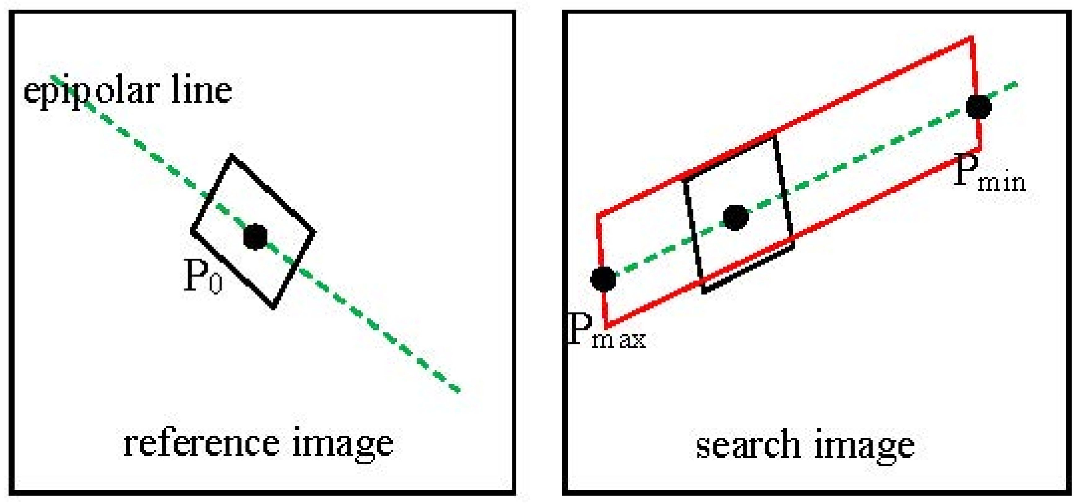
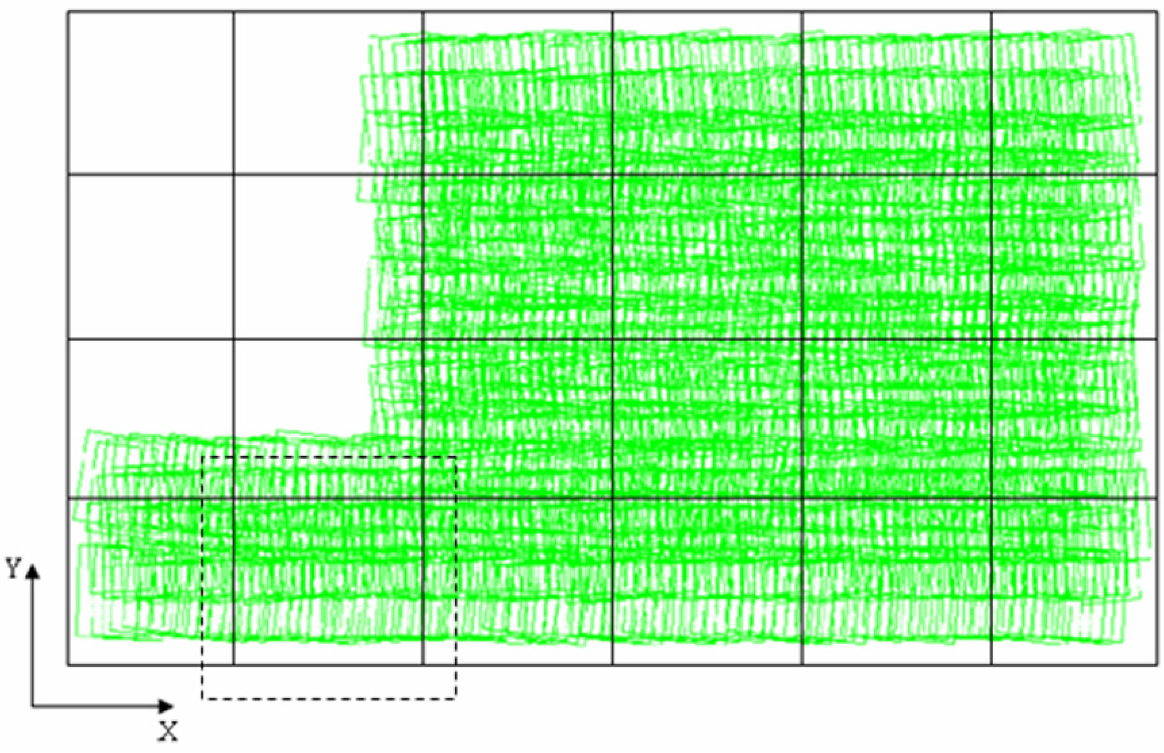
The proposed method followed PMVS by setting up regular grids on all of the images, used Harris and DOG operators to detect feature points, and then matched the feature points. For each matched feature point in the reference image, when finding candidate matching points on the corresponding epipolar line in the search image, there is an improvement compared to PMVS. In general cases, the rough ground elevation scope of the region photographed by UAV is known. Denoting the rough ground elevation scope by , there is a corresponding scope denoted by in the epipolar line of the search images; thus, we can simply seek the corresponding image points in that scope. Taking into account that the orientation elements of the reference image may not be very accurate, the search range (the red box in Figure 1) was expanded to two pixels around the epipolar line. Then, we calculated the correlation coefficient between each potential candidate matching point in that scope and the matched feature point . Because of the unstable flight attitudes of the UAV, the image deformation is large. It is not advisable to use the traditional correlation coefficient calculation method that assumes the relevant window may be simply along the direction of the image. Thus, we designed the relevant window along the direction of the epipolar line; that is to say, the edge of the relevant window was parallel with the epipolar line (Figure 1).

Figure 1.
The relevant window (black window) is consistent with the direction of the epipolar line (green dotted line).
Figure 1.
The relevant window (black window) is consistent with the direction of the epipolar line (green dotted line).
The potential candidate feature point whose correlation coefficient is greater than (in this paper, we set to be 0.7) was used as candidate match point and added to set . The set was sorted according to the value of the correlation coefficient from big to small, and then, the 3D points associated with the pairs were triangulated. According to [18], we considered these 3D points as potential patch centers. Next, we refined and verified each patch candidate associated with the potential patch center in turn according to the PMVS method. Finally, we obtained the accurate 3D seed points with normal vectors.
Edge feature detection and matching, taking the method of Li Zhang [51] as a reference, first used the Canny operator [56] to detect edge points on every image, and then performed a match for the dominant points and well-distributed points on the edges. The only difference was that after obtaining the 3D edge points using the method of [51], we used the PMVS method to refine and verify each 3D edge point.
2.3.2. Matching Propagation Based on Self-Adaptive Patch
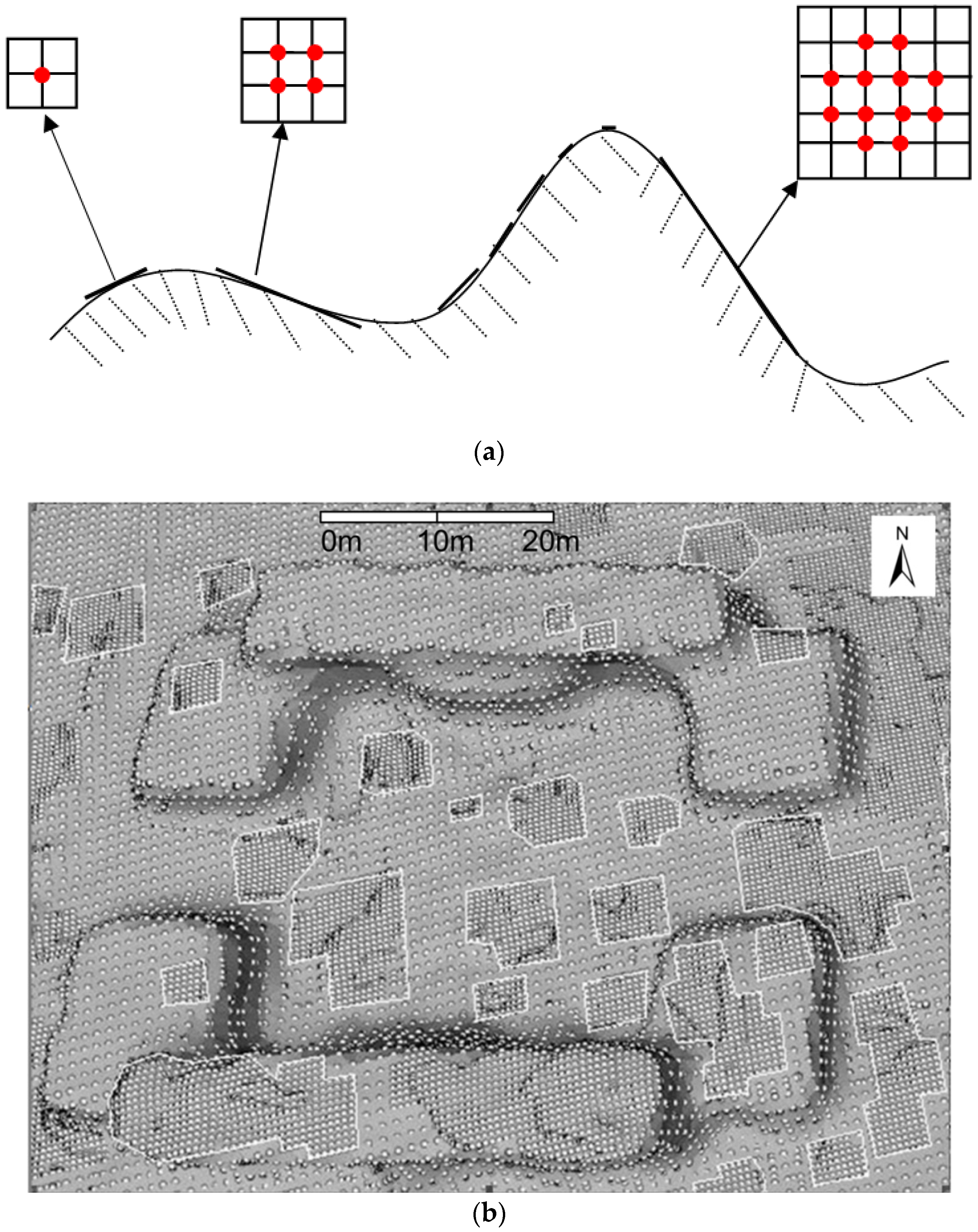
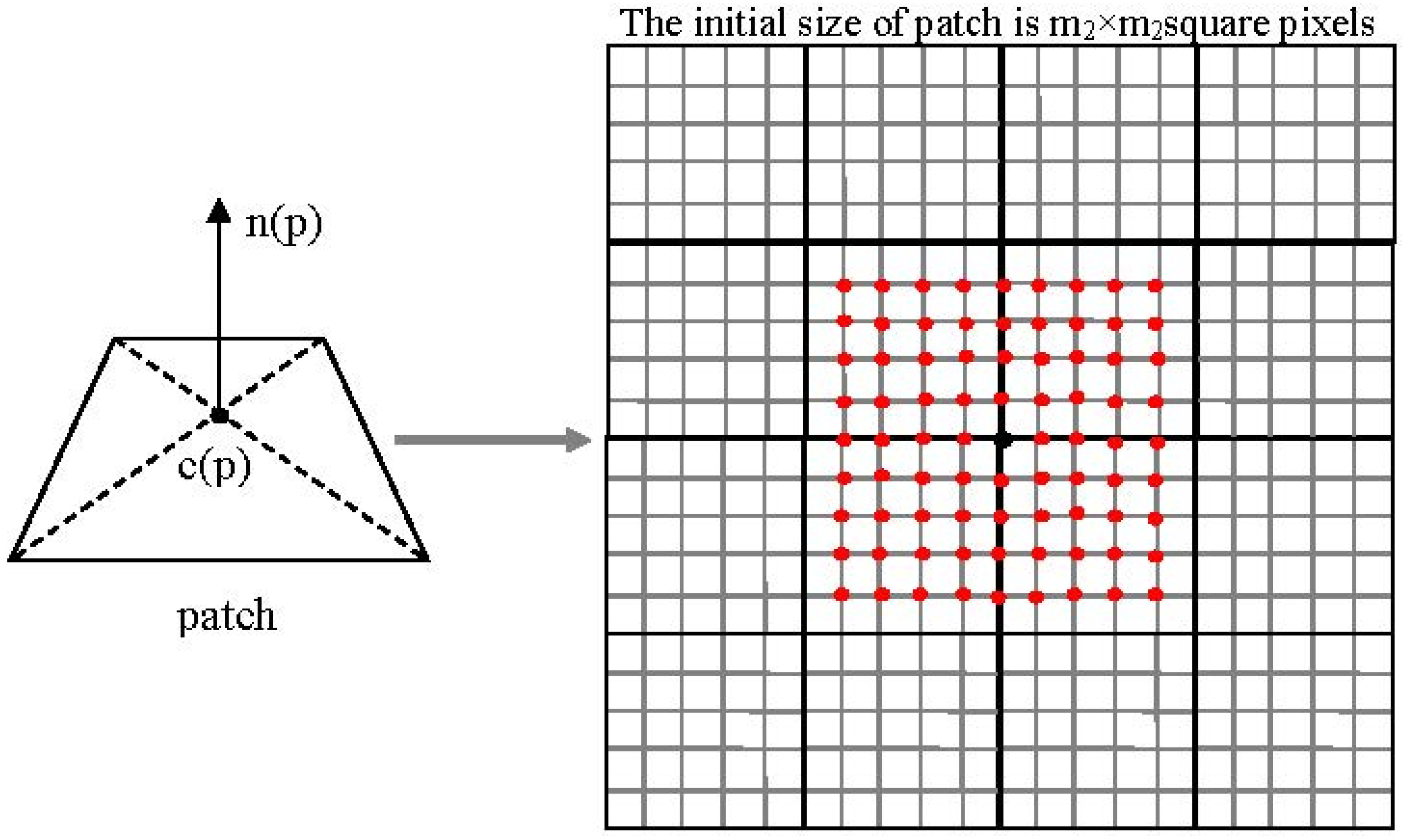
In PMVS, the 3D seed points are very sparse, and dense matching mainly depends on the expansion step; moreover, it is time-consuming. However, such speed makes it difficult to meet the requirements of real-time and convenient UAV photogrammetry. Thus, this paper presented matching propagation based on the self-adaptive patch method to improve processing efficiency. The basic concept was to build initial patches centered by the 3D seed points that had already been obtained. The extents and shapes of the patches could adapt to the terrain relief automatically: When the surface was smooth, the size of the patch would become bigger to cover the entire smooth area; if the terrain was very rough, the size of the patch would become smaller to describe the details of the surface (Figure 2a). In Figure 2, different sizes and shapes of patches are conformed to the different terrain features. There are more spread points on the larger extent patches.

Figure 2.
(a) Self-adaptive patch; (b) Schematic diagram of self-adaptive patches on the DSM.
Figure 2.
(a) Self-adaptive patch; (b) Schematic diagram of self-adaptive patches on the DSM.
The initial size of a patch must ensure that the projection of the patch onto the reference image can cover the size of square pixels (in this paper, is also denoted as the length of the patch, and the initial value of is , meaning it is three times the initial patch size of PMVS). There was an affine transformation between the patch and its projection onto the image, and the affine transformation parameters could be determined by the center coordinate and normal vector of the patch. Taking the projection of the patch onto the image as a relevant window, the correlation coefficient between the reference image and each search image donated by was calculated. Because UAV imagery is generally taken by an ordinary non-metric digital camera, the imagery usually has three channels: R, G, B. Thus, when calculating the correlation coefficient , we made full use of the information of the three channels. The formula is as follows:
where
Then, we computed the average value of the correlation coefficients as follows:
where is the number of search images.
If the is greater than the threshold , the surface area covered by the patch is smooth and can be similarly treated as a plane, so that some new 3D points (near the patch center) in the patch plane can be directly generated. The normal vectors of the new 3D points are the same as the normal vector of the patch. According to the properties of affine transformation, a plane through affine transformation becomes another plane , and the affine transformation parameters for each point on the plane are the same [18,57]; thus, we can compute the corresponding coordinates of the 3D new points in the patch by using the center point coordinate and normal vector of this patch plane. The calculation process is as follows:
- (1)
- Calculate the xyz-plane coordinate system of the patch, that is the x-axis is and the y-axis is , and the normal vector of the patch is seen as the z-axis (Figure 3). The patch center is considered the origin of the xyz-plane coordinate system of the patch. The y-axis is the vector that is perpendicular to the normal vector and the Xc-axis of the image space coordinate system; thus, . The x-axis is the vector that is perpendicular to the y-axis and the normal vector ; thus, . Then, and are normalized to the unit vector.
- (2)
- Calculate the ground resolution of the image as follows:where represents the distance between the patch center and the projection center of the image, represents the focal length, represents the angle between the light through the patch center and the normal vector of the patch, and actually represents the corresponding distance in the direction of for one pixel in the image.
- (3)
- Suppose a new point’s plane coordinate in the patch plane coordinate system is . The plane coordinates of the new points in the patch plane coordinate system are as shown in Figure 4. To ensure matching accuracy, the spread size is in the range of (the patch size is ) when the patch center is considered the origin of the patch plane coordinate system.
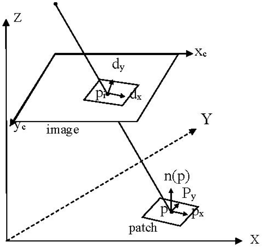
Figure 3.
The xyz-plane coordinate system of the patch.
Figure 3.
The xyz-plane coordinate system of the patch.

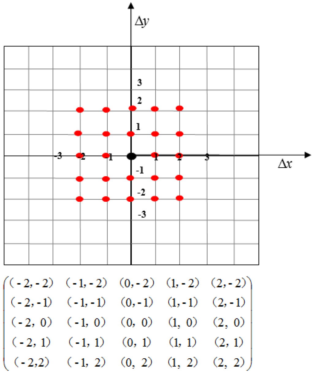
Figure 4.
The plane coordinates of the new points (red points) in the patch plane.
Figure 4.
The plane coordinates of the new points (red points) in the patch plane.

- (4)
- Calculate the XYZ-coordinate of the new point in the object space coordinate system. Suppose a (3D) new point is and the patch center is . We calculate the XYZ-coordinate of the new point as follows:
After obtaining the XYZ-coordinate of a new point in the object space coordinate system, the new point is projected onto the reference image and search images so that we can obtain the corresponding image points.
As a result, new 3D points are spread by the 3D seed point, as shown in Figure 5.

Figure 5.
The new 3D points (red points) are propagated by the seed point (black point).
Figure 5.
The new 3D points (red points) are propagated by the seed point (black point).
In our method, the size and shape of the patch can self-adapt to the texture feature: (1) For big and very smooth areas, the generated new 3D points will be directly added to the seed point set, and the newly added seed points are also in the original patch plane and they can spread further so that it enlarges the size of the original patch. Thus, the shape formed by all the spread points in the original patch would not be a regular square (Figure 2); (2) For discontinuous terrain, the length of the patch would be shortened to avoid crossing the edge, resulting in a smaller spread size (the spread size is in the range of ) and a smaller size of the patch (); (3) For a large relief terrain, the size and shape of the patch would be automatically shrunk from different directions, resulting in a smaller spread size. For such cases, the generated new 3D points would be processed following the method of PMVS. First, they are refined and verified one by one, and then the 3D points that are successfully constructed are added to the 3D seed point set. The newly added seed points are not in the original patch plane, and, thus, they will not enlarge the size of the original patch.
2.3.3. The Strategy of Matching Propagation
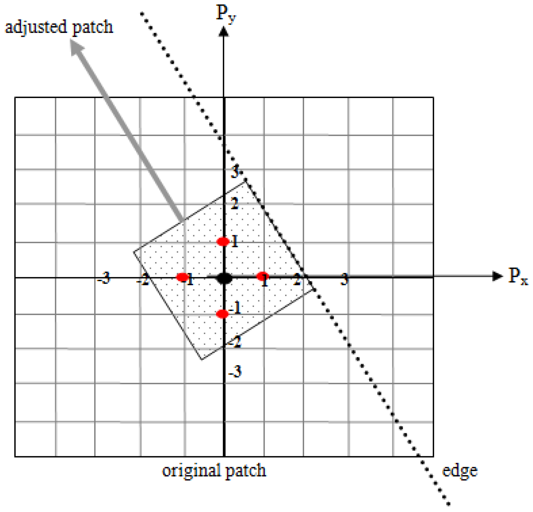
In Self-Adaptive Patch-based Multi-View Stereo-matching (SAPMVS), the size and shape of the patch should adapt to the texture feature: increasing the patch size in smooth areas and decreasing the patch size in undulating terrain. In addition, the patch should avoid crossing discontinuous terrain. The strategy of matching propagation based on the self-adaptive patch is as follows (Figure 6):
- (1)
- Get a 3D seed point from the initial feature-matching set , and build a patch by using that point as the patch center. The initial size of the patch should ensure that the projection of the patch onto the reference image is of size square pixels. In this paper, is also denoted as the length of the patch, and the initial value of is 21. However, if the set becomes empty, stop the whole matching propagation process.
- (2)
- If the patch does not contain any edge points, go to step 3. Otherwise, adjust the size and shape of the patch so that the edge (we used the edge points to determine the edge) is not crossed. In Figure 7, the patch is partitioned into two parts by an edge. We need to build a new patch from the part that contains the center point. The center point of the new patch is unchanged, and the shape is a square. One edge of the new patch is parallel to the edge. Thus, the length of the patch decreased and the shape also changed. Finally, go to step 3.
- (3)
- Take the projection of the patch onto each of the images as the relevant window, and use Equation (1) to calculate the correlation coefficient between the reference image and each search image. Then, use Equation (2) to calculate the average value of the correlation coefficients .
- (4)
- If , the size of the patch needs to be adjusted; thus, go to step 5, or else generate some new 3D points near the patch center in the range of on the patch plane. Details are presented in Section 2.3.2. Here, we need to judge whether another point has already been generated in that place. The judging method is as follows: project the new point onto the target image; if there is another point in the image pixel of the new point, give up the newly generated point. Directly add the remaining new points to the set , and go to step 1.
- (5)
- From one direction (e.g., the right), shrink the patch once by two pixels and calculate the in the meantime. If the value of is increased, continue to shrink the size of the patch in the same direction; otherwise, change the direction (e.g., left, up and down) to shrink the patch. The process above continues until . However, if the process continues until , go to step 1. After finishing the size and shape adjustment process, if the length of the patch is greater than pixels, go to step 4, or else go to step 6).
- (6)
- Generate new 3D points near the patch center in the range of on the patch plane (if , the scope becomes ). Then, refine and verify them one by one. Add the points that are constructed successfully to the set , and go to step 1.
In the end, filter the incorrect points following the PMVS filtering method.
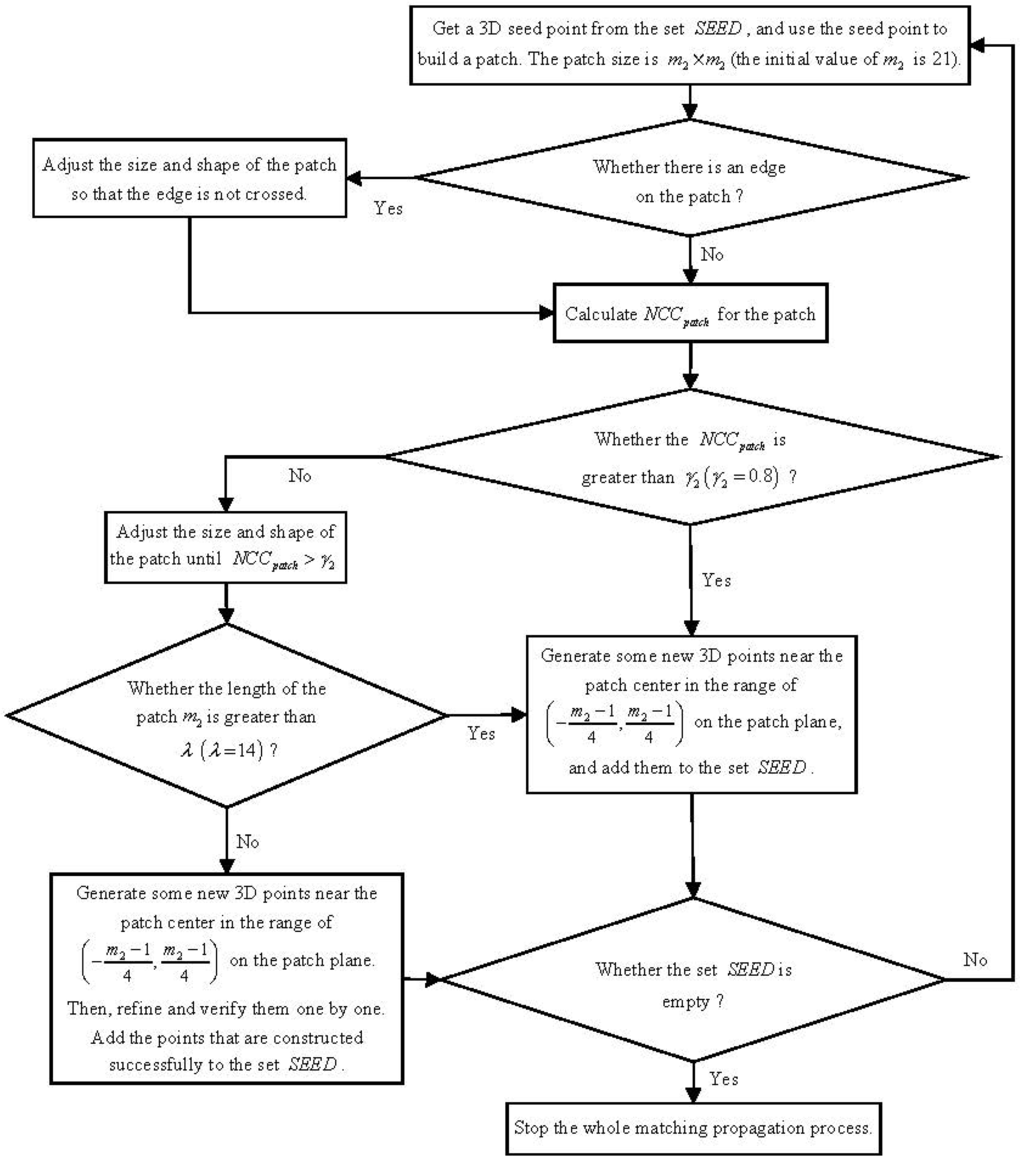
Figure 6.
The flow chart of the matching propagation based on self-adaptive patch.
Figure 6.
The flow chart of the matching propagation based on self-adaptive patch.
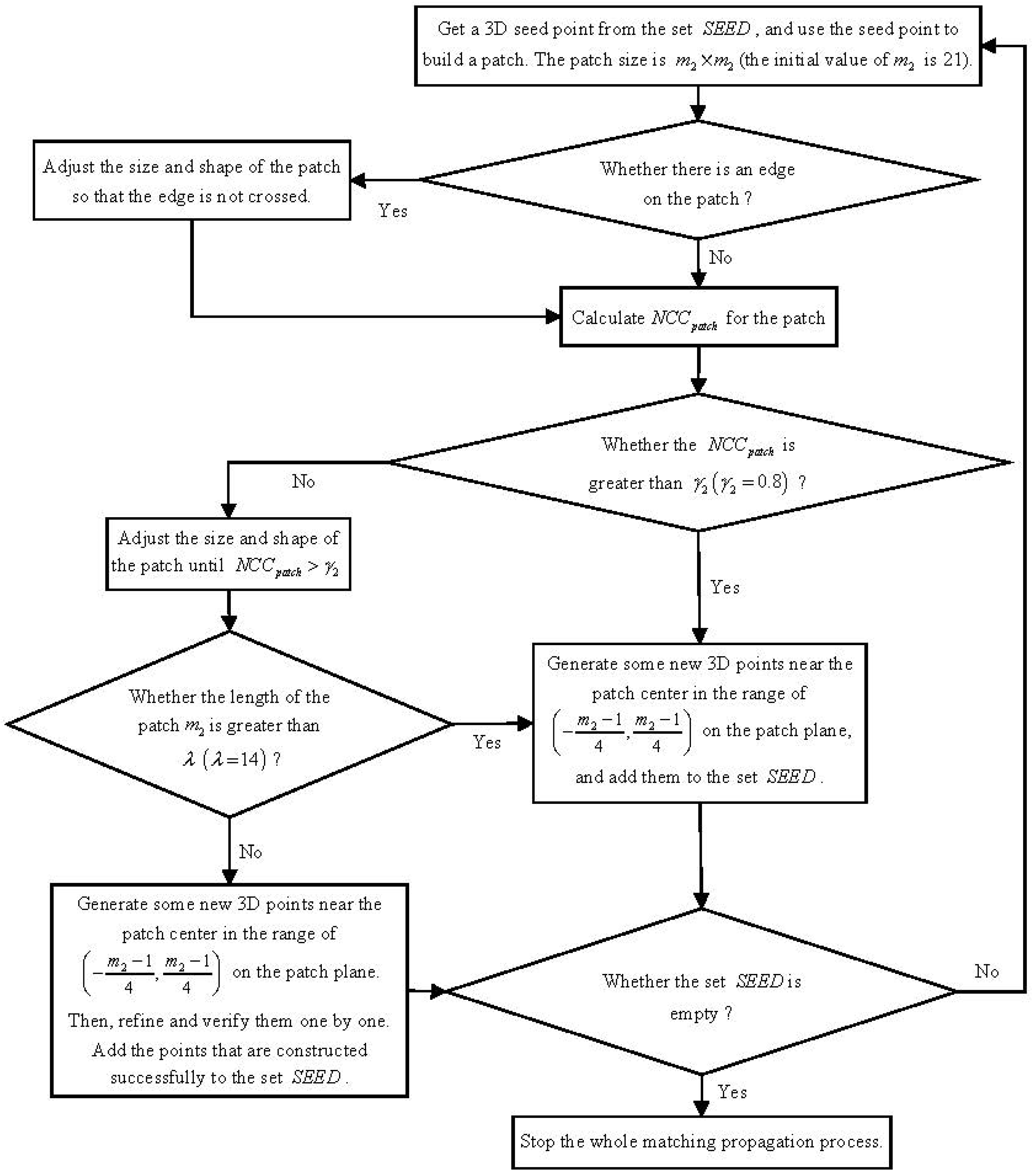

Figure 7.
Adjusting patch according to the edge.
Figure 7.
Adjusting patch according to the edge.
2.3.4. Image-Grouping
Generally, a UAV flight varies between one and three hours. The number of images can reach from 1000 to 2000. It demands a high-performance computer and, in particular, a memory with large capacity. Thus, we should divide the whole region into small regions and process each separately. Finally, combine the matching result of each image group into a whole point cloud. When we divide the whole region, we must not only consider the memory constraint but also process more images at one time. Suppose the number of images in each group is no more than (the value of is related to the computer memory and the size of the image; in this paper, ). The process for grouping images is as follows:
- (1)
- Calculate the position and the size of the associated area (footprint) of every image, that is the corresponding ground points’ XY-plane coordinates for the four corner points of the image.
Firstly, compute the size of the footprint (the length and width of the ground region) as follows:
where and are the width and height of the image. is the flight height relative to the ground, and is the focal length of the image.
Then, compute the four XY-plane coordinates of the footprint as follows:
where is the rotation angle of the image, and is the coordinate of the projection center.
- (2)
- Compute the minimum enclosing rectangle of the entire photographed area according to the footprints of all the images.
- (3)
- Divide the minimum enclosing rectangle into blocks to ensure the number of images that are completely within each block is no more than but close to (Figure 8). Compute the footprint of each block, and enlarge the block. In Figure 8, the black dotted box represents the enlarged block, which is denoted by bigBlock.
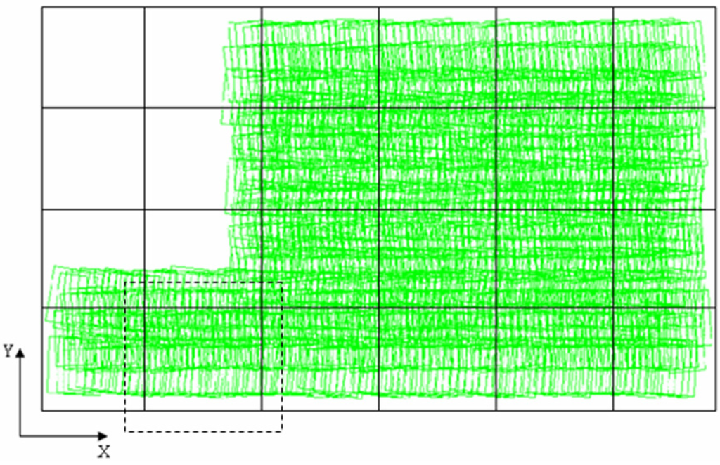
Figure 8.
To set up regular grids in a minimum enclosing rectangle.
Figure 8.
To set up regular grids in a minimum enclosing rectangle.
- (4)
- According to the footprint of every image and the footprint of every bigBlock, take all the images belonging to one bigBlock as a group.
2.3.5. Group Matching and Merging the Results
Process each image group in turn using the proposed Self-Adaptive Patch-based Multi-View Stereo-matching algorithm (SAPMVS). SAPMVS is partitioned into three parts: (1) multi-view initial feature-matching, which is introduced in Section 2.3.1; (2) matching propagation based on the self-adaptive patch, which is introduced in Section 2.3.3; (3) filtering the erroneous matching points following the PMVS filtering method. As a result, we obtain the group matching results.
Finally, we need to merge all group matching results into a whole. The merge process is as follows: (1) Remove the redundant points in bigBlock; that is, retain only the points in the block and abandon the points that exceed the extent of the block; (2) Obtain the final point cloud of the entire photographed area by merging the point clouds of every block.
To avoid gaps that appear on the edges of the blocks in the final result, in step (1) we should preserve the (3D) edge points of each block and, in step (2) remove the (3D) repetitive points at the block edges according to the corresponding image points of those 3D points. If there is a corresponding image point that belongs to two 3D points, we preserve only one of the two 3D points (or refine and verify the 3D repetitive points following the PMVS method).
3. Experiments and Results
3.1. Evaluation Index and Method
Currently, there is no unified approach to evaluating multiple image dense matching algorithms. Usually, we can compare them in the following aspects [58]: (1) accuracy, which indicates the degree of correct matching quantitatively; (2) reliability, which represents the degree of precluding overall classification error; (3) versatility, the ability to apply the algorithm to different image scenes; (4) complexity, the cost of equipment and calculation.
In the field of computer vision, to evaluate the accuracy of a multi-view dense matching algorithm, 3D reconstruction of the scene is carried out by means of the dense matching algorithm, and then the 3D reconstruction model is compared with the high-accuracy real surface model (real data are obtained by laser), and the performance of the dense matching algorithm is evaluated in terms of accuracy and completeness [17]. In the field of digital photogrammetry, we can use the corresponding image points obtained by the multi-view stereo image matching to obtain their corresponding object points by means of forward intersection, and we can then generate the Digital Surface Model (DSM) and Digital Elevation Model (DEM). Therefore, we can evaluate the accuracy of DSM and DEM and thereby evaluate the accuracy of the matching algorithm indirectly; the accuracy of the DEM and DSM can be evaluated in relation to higher-precision reference data, such as laser point cloud data and manual measurement control point data [46,51].
As the output result of our algorithm is the 3D point cloud and the computational cost is large, we will evaluate our algorithm from three aspects: visual inspection, quantitative description and complexity. Visual inspection ensures that the shape of the 3D point cloud is consistent with the actual terrain. Quantitative description is necessary to compare the 3D point cloud with the high-precision reference data, such as laser point cloud data and artificial measurement control point data. Complexity mainly refers to the requirements of devices and the cost in time of computing. On the other hand, the main input data of our algorithm are the images that have lens distortion removed [59,60,61] and their orientation elements, while the accuracy of the orientation elements can directly affect the accuracy of the imaging geometric model, which may lead to errors in the forward intersection.
3.2. Experiments and Analysis
To evaluate the performance of our multi-view stereo-matching algorithm for multiple UAV imagery in a more in-depth and comprehensive way, we will use three typical sets of UAV data with different texture features viewed from three perspectives: visual inspection, quantitative description and complexity.
3.2.1. The Experimental Platform
The proposed algorithm is implemented in Visual C++ and a PC with Intel® Core™ i7 CPU 920 2.67 GHz processors, 3.25 GB RAM, and Microsoft Windows Xp Sp3 64.
3.2.2. The First Dataset: Northwest University Campus, China
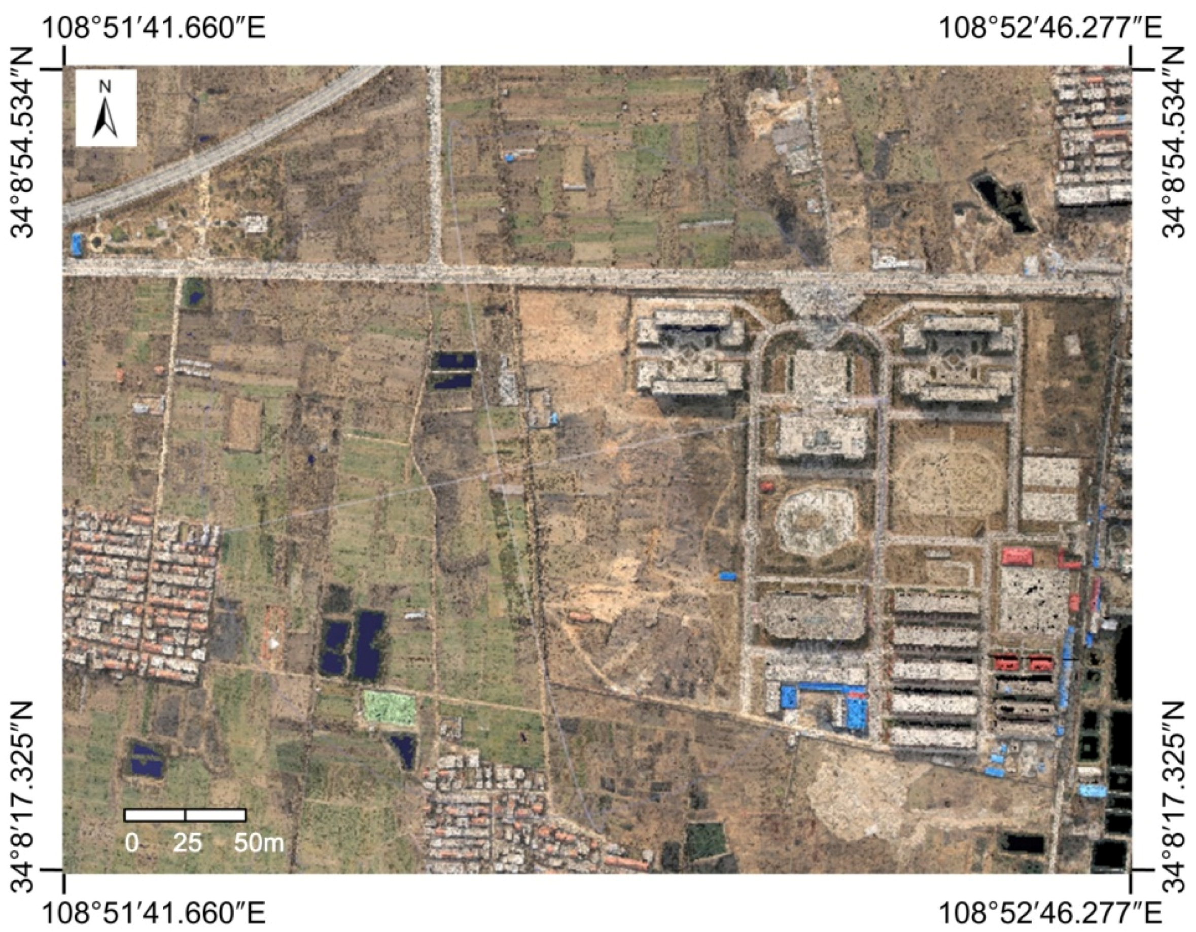
This group of experiments uses UAV imagery data taken at the Northwest University campus in Shaanxi, China, by a Cannon EOS 400D. The photography flying height is 700 m, and the ground resolution of the imagery is approximately 0.166 m. The shooting lasted 40 min, and there are a total of 67 images. The specific parameters of the photography can be seen in Table 1.

Table 1.
The parameters of the UAV photography in Northwest University.
| Camera Name | CCD Size (mm × mm) | Image Resolution (pixels × pixels) | Pixel Size (μm) | Focal Length (mm) | Flying Height (m) | Ground Resolution (m) | Number of Images |
|---|---|---|---|---|---|---|---|
| Canon EOS 400D | 22.16 × 14.77 | 3888 × 2592 | 5.7 | 24 | 700 | 0.166 | 67 |
This set of data is provided by Xi’an Dadi Surveying and Mapping Corporation. We used a commercial UAV photogrammetric processing software called GodWork, which was developed by Wuhan University, to perform automatic aerotriangulation to obtain the precise orientation elements of the images (we can also use the structure-from-motion software “VisualSFM” by Changchang Wu [62,63] to estimate the precise camera pose). The accuracy of aerotriangulation was as follows: the value of the unit-weight mean square error (Sigma0) was 0.49 pixels, and the average residual of the image point was 0.23 pixels. Because the data had no manual control point information, the bundle adjustment method and the orientation elements were under freenet. Figure 9 is the tracking map of the 67 images under freenet. We used GodWork software to remove the lens distortion of the 67 images. Table 2 shows part of the corrected images’ external orientation elements.
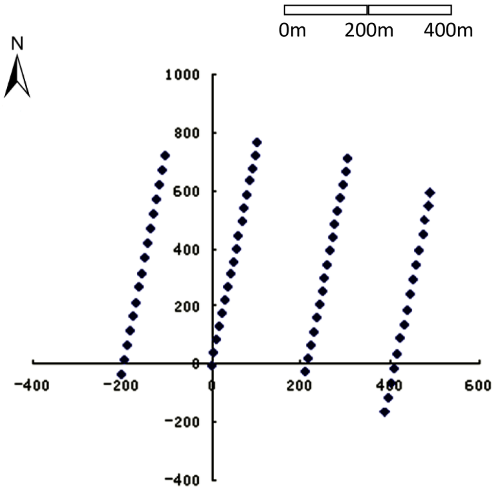
Figure 9.
The tracking map of the 67 images under freenet.
Figure 9.
The tracking map of the 67 images under freenet.
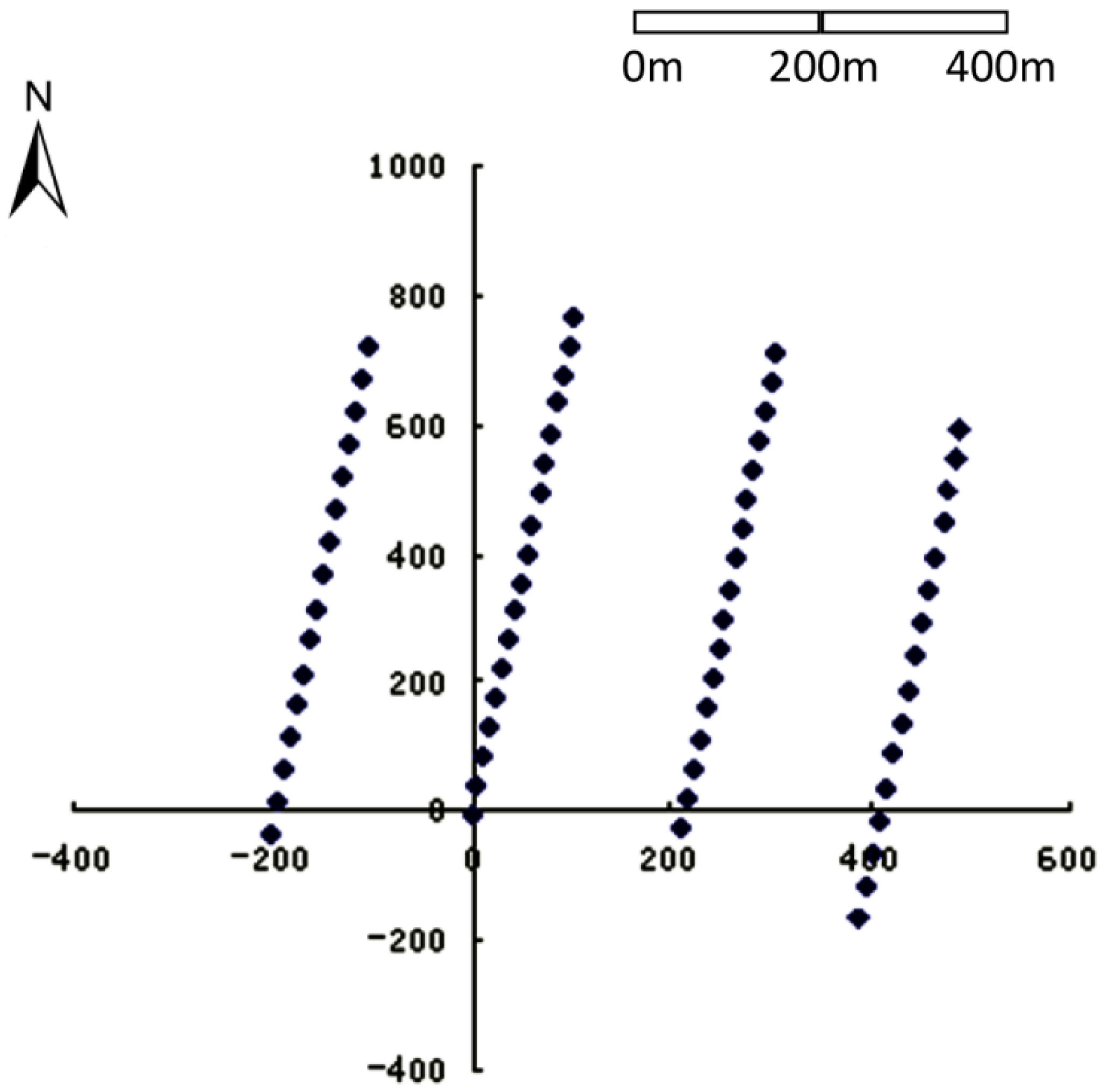
Table 2.
The external orientation elements of a portion of the corrected images.
| Image Name | X (m) | Y (m) | Z (m) | φ (Degree) | ω (Degree) | κ (Degree) |
|---|---|---|---|---|---|---|
| IMG_0555 | −201.736 | −31.7532 | −1.35375 | −1.0234 | −0.44255 | 166.7002 |
| IMG_0554 | −194.482 | 17.90618 | −1.22801 | −0.71193 | −0.1569 | 166.2114 |
| IMG_0553 | −187.641 | 67.63342 | −0.87626 | 0.320481 | −0.03621 | 166.3385 |
| IMG_0552 | −180.965 | 116.052 | −0.61774 | 0.518773 | −0.87317 | 166.7509 |
| IMG_0551 | −174.434 | 166.2001 | −0.59227 | 0.454139 | −0.86679 | 167.2784 |
| IMG_0550 | −168.264 | 214.3878 | −0.79246 | −0.57551 | −0.67894 | 167.5912 |
| IMG_0549 | −162.096 | 265.1268 | −0.70428 | −1.08565 | −0.7456 | 167.166 |
| IMG_0548 | −156.002 | 314.2426 | −0.53393 | −1.40444 | −0.84598 | 166.5402 |
| IMG_0547 | −148.987 | 367.3003 | −0.30983 | −0.77136 | −0.86104 | 166.5097 |
| IMG_0546 | −142.152 | 417.2658 | −0.04708 | −0.38776 | −0.89084 | 166.5219 |
| IMG_0545 | −135.102 | 466.7365 | 0.507349 | −0.08542 | −0.09929 | 166.4838 |
| IMG_0544 | −128.322 | 520.032 | 1.246216 | −0.2938 | −0.41415 | 166.7157 |
| IMG_0543 | −121.833 | 569.8722 | 1.862483 | −0.20825 | −0.21687 | 167.1119 |
First, we used the proposed UAV multiple image–grouping strategy to divide this set of 67 images into 12 groups. The serial number of each image group is shown in Table 3.
Table 3.
Image-grouping result of the Northwest University data.
| Group | Image Number | Corresponding Image Name | Number of Images |
|---|---|---|---|
| 0 | 0 1 2 3 4 5 | IMG_1093~IMG_1089 | 6 |
| 1 | 6 7 8 9 10 11 | IMG_ 1087~IMG_1082 | 6 |
| 2 | 12 13 14 15 | IMG_1081~IMG_1078 | 4 |
| 3 | 16 17 18 19 20 21 | IMG_0102~IMG_0107 | 6 |
| 4 | 22 23 24 25 26 27 | IMG_0108~IMG_0113 | 6 |
| 5 | 28 29 30 31 32 | IMG_0114~IMG_0118 | 5 |
| 6 | 33 34 35 36 37 38 | IMG_0641~IMG_0646 | 6 |
| 7 | 39 40 41 42 43 44 | IMG_0647~IMG_0652 | 6 |
| 8 | 45 46 47 48 49 50 | IMG_0653~IMG_0658 | 6 |
| 9 | 51 52 53 54 55 56 | IMG_0555~IMG_0550 | 6 |
| 10 | 57 58 59 60 61 62 | IMG_0549~IMG_0544 | 6 |
| 11 | 63 64 65 66 | IMG_0543~IMG_0540 | 4 |
After image-grouping, we used the proposed Self-Adaptive Patch-based Multi-View Stereo-matching algorithm (SAPMVS) to address each image group, and obtained the 3D dense point cloud data of each image group. Then, we merged the 3D dense point clouds of each group; the merged 3D dense point cloud is shown in Figure 10 (the small black areas in the figures are water). We found that the merged 3D dense point cloud has 8,526,192 points, and the point density is approximately three points per square meter; thus, the ground resolution is approximately 0.3 m.
Because of the lack of control point data or high-precision reference data in the data set, such as the laser point cloud, we use the visual inspection method to evaluate the results of the proposed algorithm, i.e., whether the shape of the 3D point cloud is consistent with the actual terrain. We compared the 3D dense point cloud and the corresponding corrected images that had the lens distortion removed, as shown in Figure 11. By comparing the point clouds and images in Figure 11, it can be seen that the 3D dense point clouds of the proposed algorithm accurately described the terrain features of the Northwest University campus as well as the shape and distribution of physical objects (such as roads and buildings).

Figure 10.
The merged 3D dense point cloud of Northwest University.
Figure 10.
The merged 3D dense point cloud of Northwest University.
For further analysis of the accuracy and efficiency of the proposed algorithm, we used the proposed IG-SAPMVS algorithm and PMVS algorithm [18,52], respectively, to process this set of data, and recorded the processing time and the 3D point cloud results. Table 4 shows the statistics for these two algorithms with respect to the processing time and the point number of 3D dense point clouds. Figure 12 shows the final 3D dense point cloud results.
From Table 4, it can be seen that the processing time of the proposed IG-SAPMVS algorithm is approximately 0.5 times that of the PMVS algorithm; thus, the calculation efficiency of the proposed IG-SAPMVS algorithm is significantly higher than that of the PMVS algorithm. Because the terrain relief of the test area is not large and there are many flat square grounds in the test area, the proposed Self-Adaptive Patch-based Multi-View Stereo-matching algorithm (SAPMVS) can spread more quickly than the PMVS algorithm in the matching propagation process. On the other hand, based on Table 4, it can be seen that the point number of the 3D dense point cloud by the proposed IG-SAPMVS algorithm is 1.15 times that of the PMVS algorithm; Figure 12 illustrates that the 3D dense point cloud result of the proposed IG-SAPMVS algorithm is almost the same as that of the PMVS algorithm based on visual inspection. In general, the proposed IG-SAPMVS algorithm outperforms the PMVS algorithm in computing efficiency and the quantity of 3D dense point clouds.
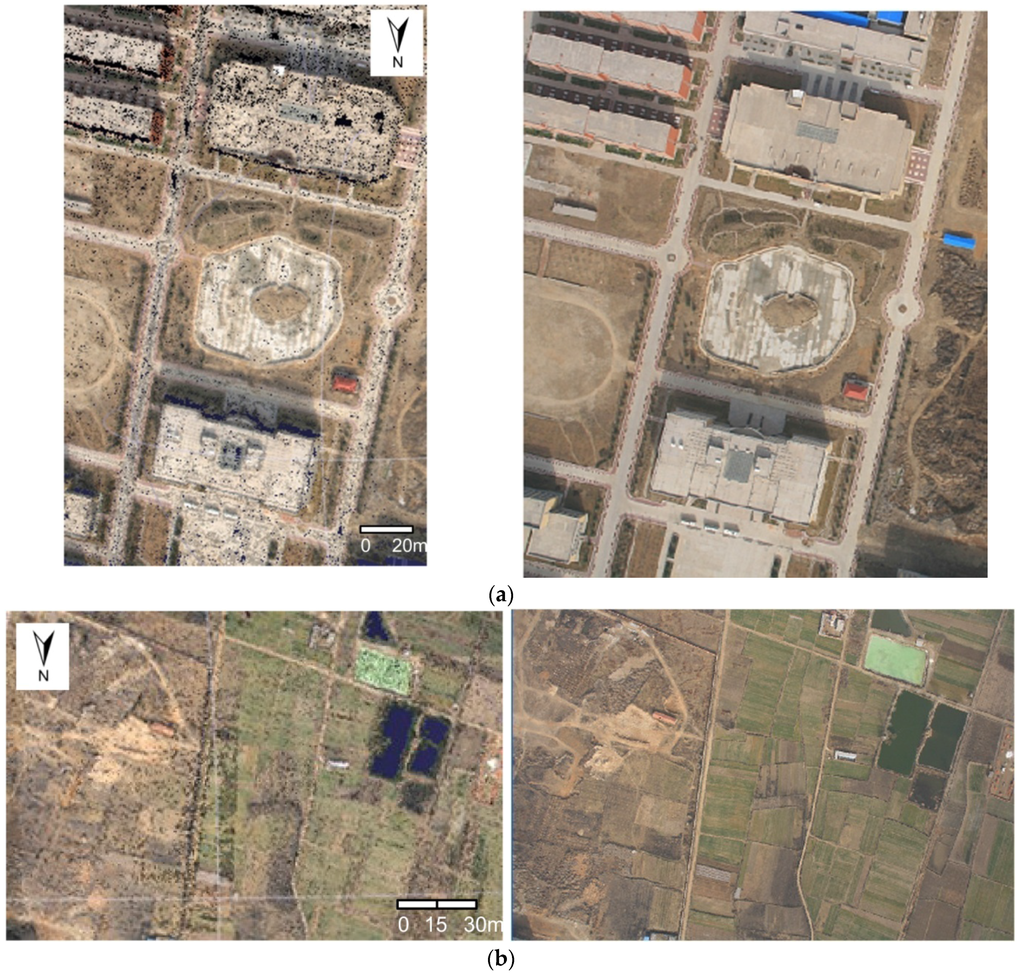
Figure 11.
Comparison of the same areas in the 3D dense point clouds and the corresponding images. (a) The building area; (b) the flat area.
Figure 11.
Comparison of the same areas in the 3D dense point clouds and the corresponding images. (a) The building area; (b) the flat area.

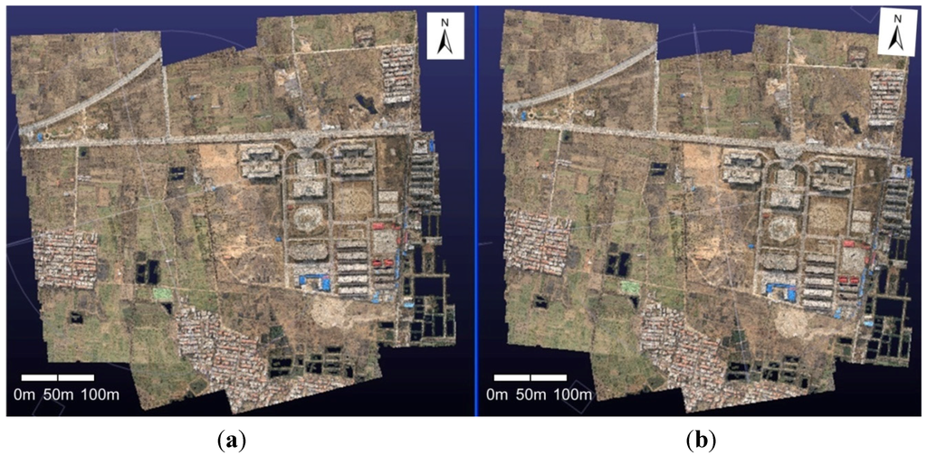
Figure 12.
Final 3D point cloud results of the Northwest University campus using IG-SAPMVS (a) and PMVS (b).
Figure 12.
Final 3D point cloud results of the Northwest University campus using IG-SAPMVS (a) and PMVS (b).
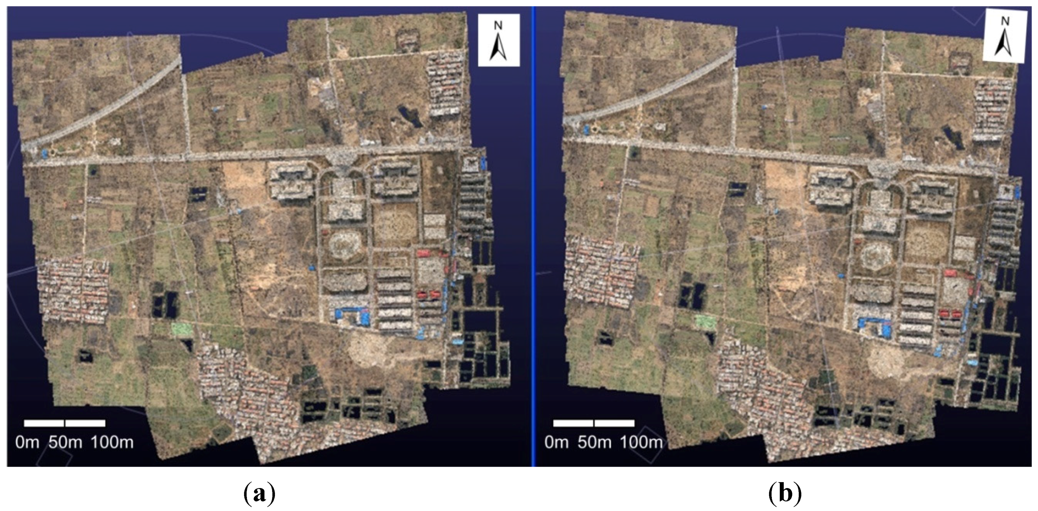
Table 4.
Statistics for the proposed IG-SAPMVS algorithm and PMVS algorithm.
| Algorithm | RunTime (h:min:s) | Point Cloud Amount | Number of Images |
|---|---|---|---|
| IG-SAPMVS | 2:41:38 | 8526192 | 67 |
| PMVS | 4:8:30 | 7428720 | 67 |
3.2.3. The Second Dataset: Remote Mountains
This group of experiments uses UAV imagery data of remote mountains characterized by large relief, heavy vegetation and a small amount of physical objects, such as roads and buildings, in China; they were also taken by a Cannon EOS 400D with a focus of 24 mm. The photography flying height is approximately 1900 m and the ground resolution of the imagery is approximately 0.451 m. There are a total of 125 images. Figure 13 is the GPS tracking map under the geodetic control network. We also used GodWork software to remove the lens distortion of the 125 images.
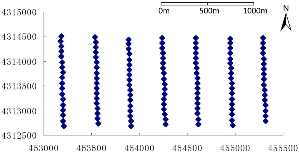
Figure 13.
The GPS tracking map of the UAV images taken in remote mountains under geodetic control network.
Figure 13.
The GPS tracking map of the UAV images taken in remote mountains under geodetic control network.

This set of data is also provided by Xi'an Dadi Surveying and Mapping Corporation. Because of the low accuracy of the airborne GPS/IMU data, it cannot meet the requirements of the proposed multi-view stereo-matching algorithm. We used the commercial UAV photogrammetric processing software GodWork, which was developed by Wuhan University, to perform automatic aerotriangulation and obtain the images’ precise exterior orientation elements. The accuracy of aerotriangulation was as follows: the value of the unit-weight mean square error (Sigma0) was 0.77 pixels, and the average residual of the image point was 0.36 pixels. Table 5 shows part of the corrected images’ external orientation elements.
First, we also used the UAV multiple image-grouping strategy to divide this set of 125 images into 21 groups. After image-grouping, we used the proposed Self-Adaptive Patch-based Multi-View Stereo-matching algorithm (SAPMVS) to address each image group, and obtained the 3D dense point cloud data of each image group. Then, we merged the 3D dense point clouds of each group, and the merged 3D dense point cloud is shown in Figure 14 (the small black areas in the figures are water). We found that the merged 3D dense point cloud has 12,509,202 points, and the point density is approximately one point per square meter; thus, the ground resolution is approximately 1 m.
Table 5.
The external orientation elements of part of the corrected images (the remote mountains).
| Image Name | X (m) | Y (m) | Z (m) | φ (Degree) | ω (Degree) | κ (Degree) |
|---|---|---|---|---|---|---|
| IMG_0250 | 453208.9 | 4312689 | 1926.36 | 4.251745 | −2.30691 | 10.23632 |
| IMG_0251 | 453205.6 | 4312796 | 1926.462 | 2.852207 | −6.04494 | 10.94959 |
| IMG_0252 | 453200.6 | 4312900 | 1921.71 | 0.681977 | −7.93856 | 11.60872 |
| IMG_0253 | 453198.6 | 4313007 | 1920.499 | −0.01863 | −3.6135 | 8.714555 |
| IMG_0254 | 453198.7 | 4313117 | 1915.972 | 3.277204 | −6.38877 | 8.599633 |
| IMG_0255 | 453199.3 | 4313230 | 1910.448 | 6.64432 | −6.29777 | 8.965715 |
| IMG_0256 | 453196.7 | 4313341 | 1904.105 | 3.33602 | −6.5811 | 10.72329 |
| IMG_0257 | 453194.1 | 4313450 | 1903.386 | 1.594531 | −4.486 | 10.71933 |
| IMG_0258 | 453192.8 | 4313559 | 1902.593 | −4.04339 | −5.57166 | 8.112464 |
| IMG_0259 | 453194.9 | 4313667 | 1899.551 | 3.77633 | −2.96418 | 7.066141 |
| IMG_0260 | 453198.2 | 4313776 | 1899.075 | 7.240338 | −5.29839 | 8.254281 |
| IMG_0261 | 453196.6 | 4313882 | 1898.725 | 3.41796 | −1.02482 | 10.90049 |
| IMG_0262 | 453193.1 | 4313986 | 1895.928 | 3.000324 | −5.9483 | 12.35882 |
| IMG_0263 | 453185.4 | 4314095 | 1896.413 | 1.532879 | −4.00544 | 11.27756 |
| IMG_0264 | 453184 | 4314196 | 1895.204 | 4.379199 | −2.4512 | 11.95034 |

Figure 14.
The merged 3D dense point cloud of the remote mountains. (a) The plan view of the merged 3D dense point cloud; (b) The side views of the merged 3D point-cloud.
Figure 14.
The merged 3D dense point cloud of the remote mountains. (a) The plan view of the merged 3D dense point cloud; (b) The side views of the merged 3D point-cloud.
For further analysis of the accuracy and efficiency of the proposed algorithm, we used the proposed IG-SAPMVS algorithm and PMVS algorithm [18,52], respectively, to process this set of remote mountain data and recorded the processing time and the 3D point cloud results. Table 6 shows the statistics of these two algorithms with respect to the processing time and the point number of the 3D dense point clouds. Figure 15 shows the final results of the 3D dense point cloud.
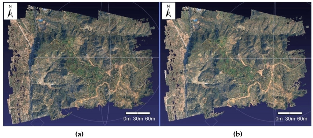
Figure 15.
Final 3D point cloud results of the remote mountains using IG-SAPMVS (a) and PMVS (b).
Figure 15.
Final 3D point cloud results of the remote mountains using IG-SAPMVS (a) and PMVS (b).
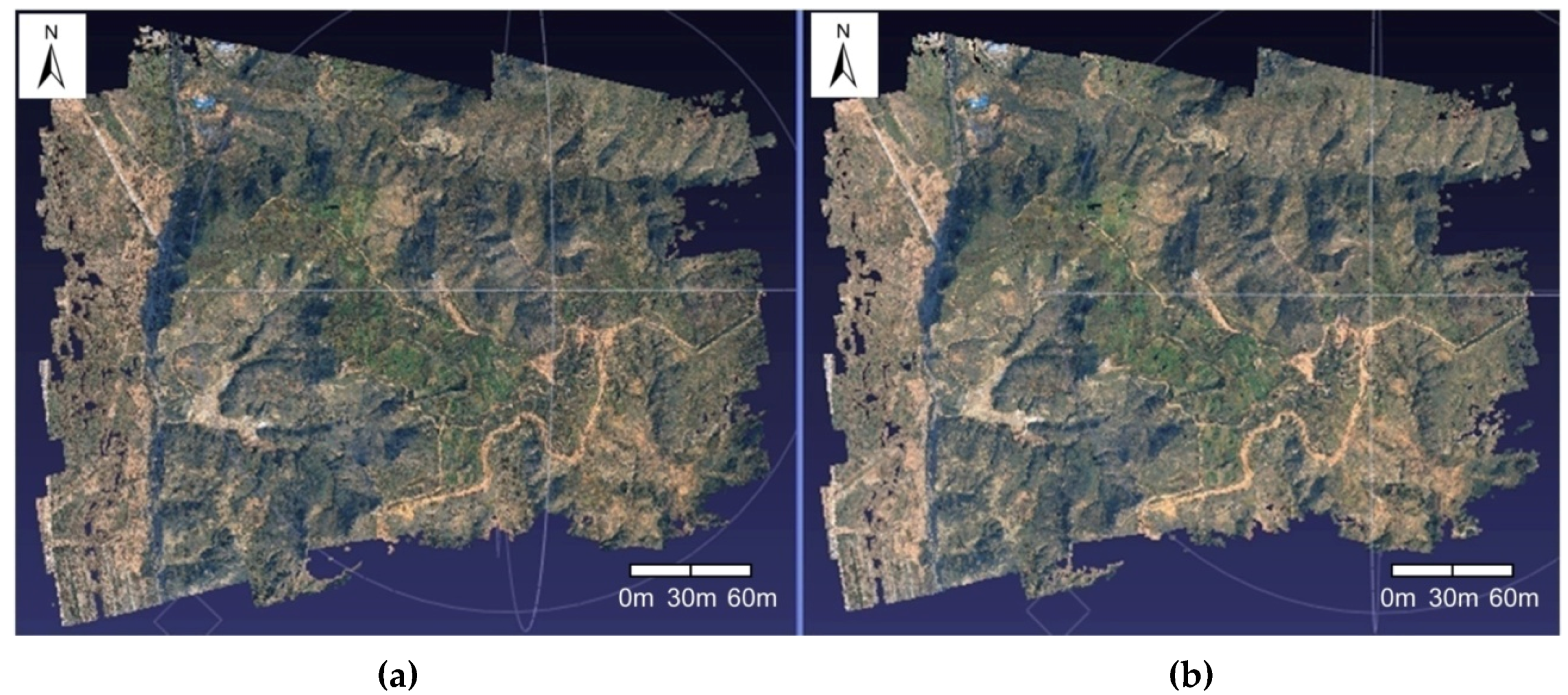
Table 6.
The statistics of the proposed IG-SAPMVS algorithm and PMVS algorithm.
| Algorithm | RunTime (h:min:s) | Point Cloud Amount | Number of Images |
|---|---|---|---|
| IG-SAPMVS | 4:36:5 | 12509202 | 125 |
| PMVS | 15:48:11 | 8953228 | 125 |
From Table 6, it can be seen that the processing time of the proposed IG-SAPMVS algorithm is about one-third of that of the PMVS algorithm; thus, the efficiency of the proposed IG-SAPMVS algorithm is significantly higher than that of the PMVS algorithm. Obviously, even in the remote mountain field with complex terrain, the proposed Self-Adaptive Patch-based Multi-View Stereo-matching algorithm (SAPMVS) can spread more quickly than the PMVS algorithm in the matching propagation process. On the other hand, based on Table 6, it can be seen that the point number of the 3D dense point cloud by the proposed IG-SAPMVS algorithm is 1.40 times that of the PMVS algorithm, and Figure 15 illustrates that the 3D dense point cloud result of the proposed IG-SAPMVS algorithm is nearly the same as the PMVS algorithm based on visual inspection. In general, the proposed IG-SAPMVS algorithm significantly outperforms the PMVS algorithm in computing efficiency and the quantity of 3D dense point clouds.
3.2.4. The Third Dataset: Vaihingen, Germany
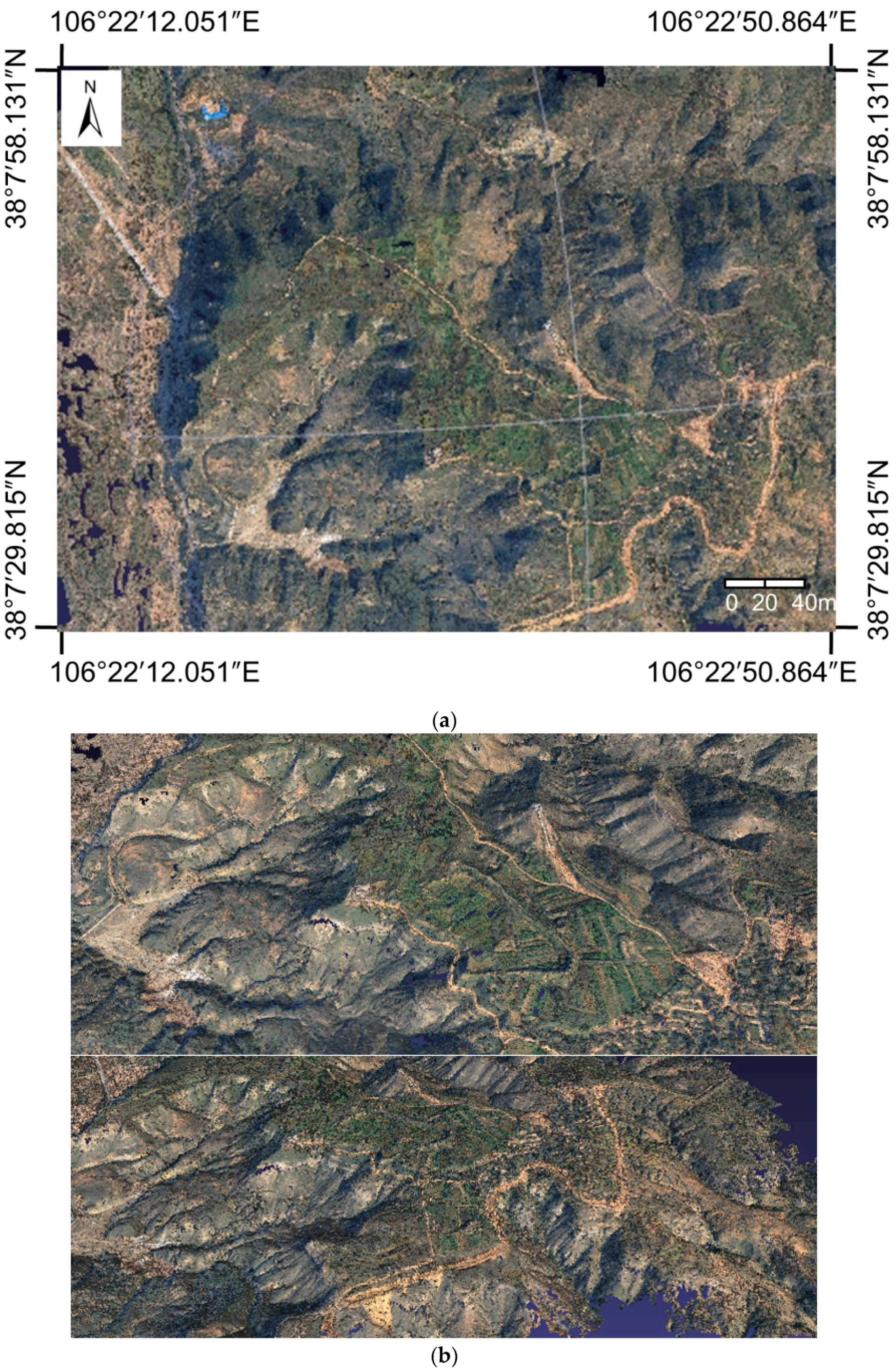
The third dataset was captured over Vaihingen, Germany, by the German Society for Photogrammetry, Remote Sensing and Geoinformation (DGPF) [64]. It consists of three test areas of various object classes (three yellow areas in Figure 16).
- •
- Area 1 “Inner City”: This test area is situated in the center of the city of Vaihingen. It is characterized by dense development consisting of historic buildings with rather complex shapes, but there are also some trees (Figure 17a).
- •
- Area 2 “High Riser”: This area is characterized by a few high-rise residential buildings that are surrounded by trees (Figure 17b).
- •
- Area 3 “Residential Area”: This is a purely residential area with small detached houses (Figure 17c).

Figure 16.
The Vaihingen test areas.
Figure 16.
The Vaihingen test areas.
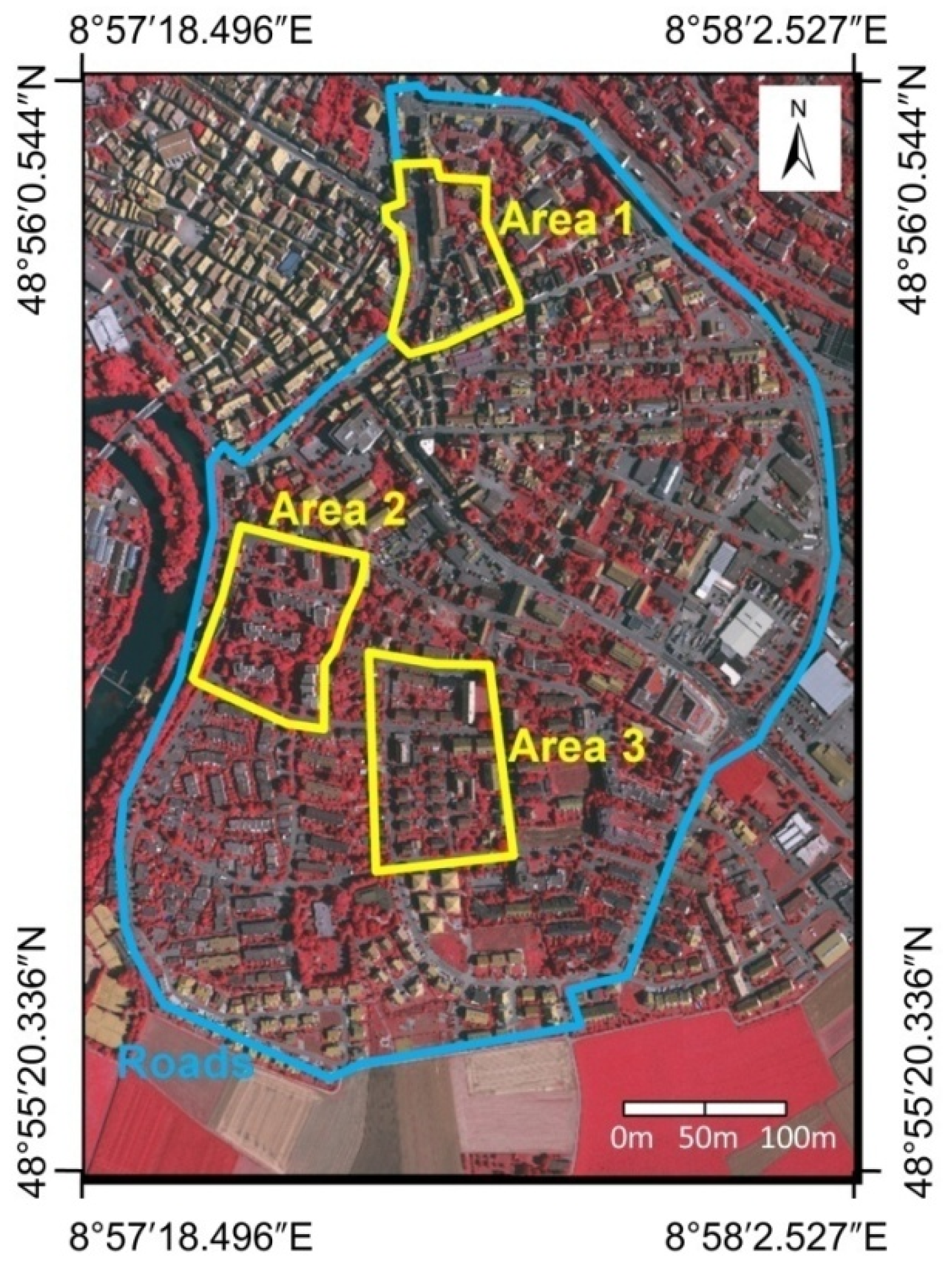
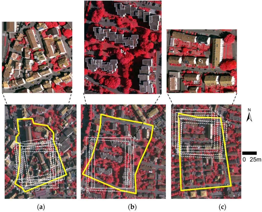
Figure 17.
The three test sites in Vaihingen. (a) a1-a8: the eight cut images of the “Inner City” from the original images: 10030061.jpg, 10030062.jpg, 10040083.jpg, 10040084.jpg, 10050105.jpg, 10050106.jpg, 10250131.jpg, 10250132.jpg, respectively; (b) b1-b4: the four cut images of the “High Riser” from the original images: 10040082.jpg, 10040083.jpg, 10050104.jpg, 10050105.jpg, respectively; (c) c1-c6: the six cut images of the “Residential Area” from the original images: 10250134.jpg, 10250133.jpg, 10040083.jpg, 10040084.jpg, 10050105.jpg, 10050106.jpg, respectively.

The data include high-resolution digital aerial images and orientation parameters and airborne laser scanner data (available in [65]).
Digital Aerial Images and Orientation Parameters: The images are a part of the Intergraph/ZI DMC block with 8 cm ground resolution [64]. Each area is visible in multiple images from several strips. The orientation parameters are distributed together with the images. The accuracy of aerotriangulation is as follows: the value of unit-weight mean square error (Sigma0) is about 0.25 pixels. Table 7 shows the external orientation elements of the images in the test region.
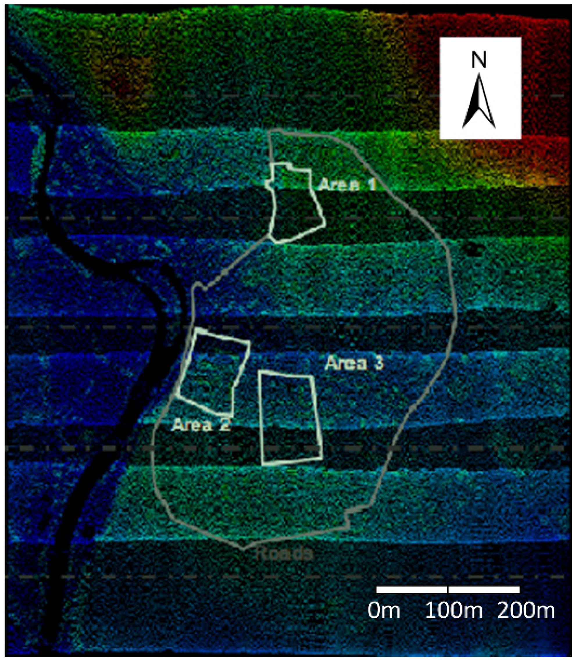
Airborne Laser Scanner Data: The test area was covered by 10 strips captured with a Leica ALS50 system. Inside an individual strip, the average point density is 4 points [66]. The airborne laser scanner data of the test region are shown in Figure 18.
Table 7.
The external orientation elements of the experimental images (Vaihingen data).
| Image Name | X (m) | Y (m) | Z (m) | ω (Degree) | ϕ (Degree) | κ (Degree) |
|---|---|---|---|---|---|---|
| 10030060.tif | 496803.043 | 5420298.566 | 1163.983 | 2.50674 | 0.73802 | 199.32970 |
| 10030061.tif | 497049.238 | 5420301.525 | 1163.806 | 2.05968 | 0.67409 | 199.23470 |
| 10030062.tif | 497294.288 | 5420301.839 | 1163.759 | 1.97825 | 0.51201 | 198.84290 |
| 10030063.tif | 497539.821 | 5420299.469 | 1164.423 | 1.40457 | 0.38326 | 198.88310 |
| 10040081.tif | 496558.488 | 5419884.008 | 1181.985 | −0.87093 | 0.36520 | −199.20110 |
| 10040082.tif | 496804.479 | 5419882.183 | 1183.373 | −0.26935 | −0.63812 | −198.97290 |
| 10040083.tif | 497048.699 | 5419882.847 | 1184.616 | 0.34834 | −0.40178 | −199.44720 |
| 10040084.tif | 497296.587 | 5419884.550 | 1185.010 | 0.81501 | −0.53024 | −199.35600 |
| 10040085.tif | 497540.779 | 5419886.806 | 1184.876 | 1.38534 | −0.46333 | −199.85010 |
| 10050103.tif | 496573.389 | 5419477.807 | 1161.431 | −0.48280 | −0.03105 | −0.23869 |
| 10050104.tif | 496817.972 | 5419476.832 | 1161.406 | −0.65210 | −0.06311 | −0.17326 |
| 10050105.tif | 497064.985 | 5419476.630 | 1159.940 | −0.74655 | 0.11683 | −0.09710 |
| 10050106.tif | 497312.996 | 5419477.065 | 1158.888 | −0.53451 | −0.19025 | −0.13489 |
| 10050107.tif | 497555.389 | 5419477.724 | 1158.655 | −0.55312 | −0.12844 | −0.13636 |
| 10250130.tif | 497622.784 | 5420189.950 | 1180.494 | 0.09448 | 3.41227 | −101.14170 |
| 10250131.tif | 497630.734 | 5419944.364 | 1181.015 | 0.61065 | 2.54420 | −97.84478 |
| 10250132.tif | 497633.024 | 5419698.973 | 1179.964 | 1.27053 | 1.62793 | −97.23292 |
| 10250133.tif | 497628.317 | 5419452.807 | 1179.237 | 0.90688 | 0.83308 | −98.72504 |
| 10250134.tif | 497620.954 | 5419207.621 | 1178.201 | 0.17675 | 1.27920 | −101.86160 |
| 10250135.tif | 497617.307 | 5418960.618 | 1176.629 | 0.22019 | 1.47729 | −101.55860 |

Figure 18.
The airborne laser scanner data of the experimental region (Vaihingen).
Figure 18.
The airborne laser scanner data of the experimental region (Vaihingen).
Because this dataset’s image pixel resolution ( square pixels) is large, it often exhausted the computer memory in the experiment when processing the original images. In addition, the imaging of any of the three experimental areas is only a small part of each image. Therefore, we can cut out the three experimental areas in each of the original images separately (Figure 17). We used the proposed Self-Adaptive Patch-based Multi-View Stereo-matching algorithm (SAPMVS) to address the three sets of cut images separately, and obtained the 3D dense point cloud data of each dataset. The 3D dense point cloud data of each dataset are shown in Figure 19. The statistics of the results by the proposed SAPMVS algorithm are shown in Table 8.

Figure 19.
Final 3D point cloud results for the three sets of cut images. (a) Area 1: “Inner City”; (b) Area 2: “High Riser”; (c) Area 3: “Residential Area”.
Figure 19.
Final 3D point cloud results for the three sets of cut images. (a) Area 1: “Inner City”; (b) Area 2: “High Riser”; (c) Area 3: “Residential Area”.
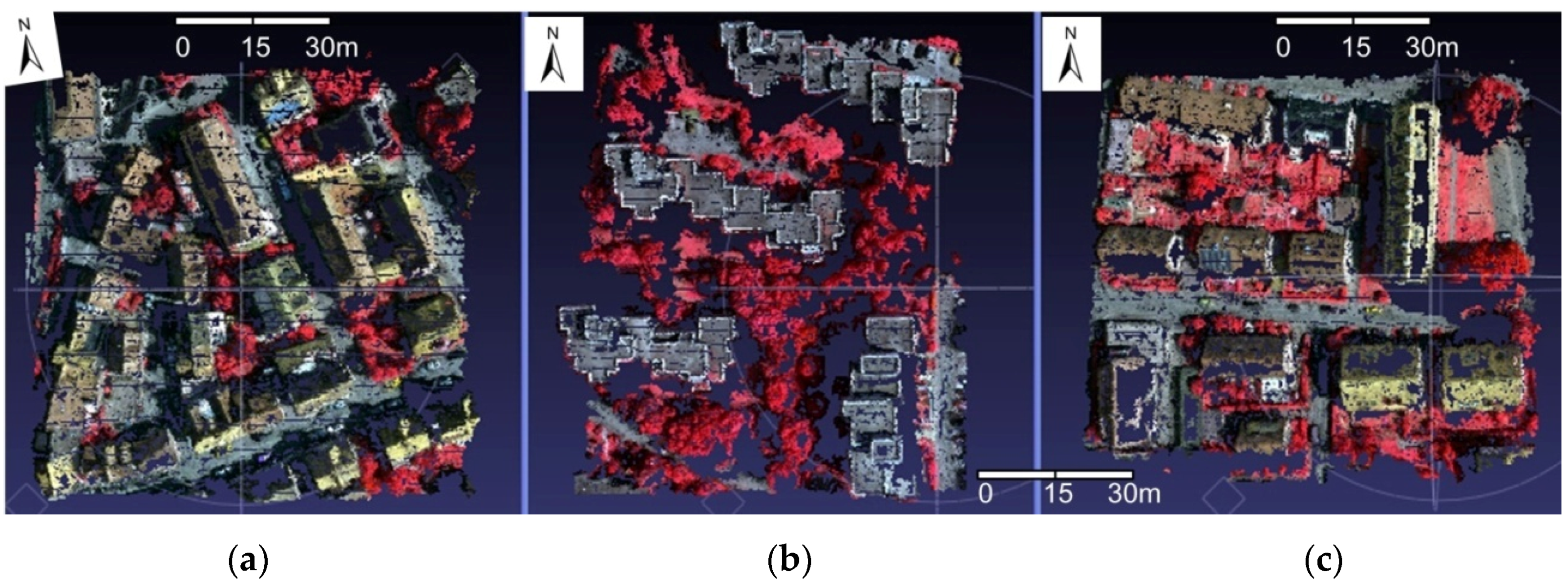
Table 8.
The statistics for the results of the Vaihingen data by the proposed SAPMVS algorithm.
| Experiment Area | Number of Images (Image Pixel Resolution) | Point Amount | Average Distance between Points | RunTime (min:s) |
|---|---|---|---|---|
| Area 1: “Inner City” | 8 (1200*1200) | 253125 | 16 cm | 11:33 |
| Area 2: “High Riser” | 4 (1200*1600) | 220073 | 16 cm | 6:30 |
| Area 3: “Residential Area” | 6 (1400*1300) | 259637 | 16 cm | 9:46 |
From Table 8 and Figure 19, it can be seen that the computational efficiency of the proposed SAPMVS algorithm is high and the ground resolution of the obtained 3D dense point cloud is approximately 0.16 m.
To quantitatively describe the accuracy of the proposed algorithm, we can compare the obtained 3D point cloud results by the PMVS and the proposed algorithm with the high-precision airborne laser scanner data, respectively. The specific evaluation method is performed as follows: For each 3D point of the obtained point-cloud result that was assumed to be , we determine all the laser points near the point (the XY-plane distance between point and the laser point should be smaller than the threshold value , which is related to the average point density of the airborne laser scanner data, in our experiment ) in the laser point cloud data; we then calculate the average elevation of these nearby laser points as the reference elevation of the point [36]. Finally, we compare the elevation of the point with its reference elevation and calculate the root mean square error () and the maximum error () of the obtained 3D point cloud [67]. The calculation formulas are as follows:
where represents the point number of the obtained 3D dense point cloud result. It should be noted that using this method to evaluate the accuracy of the obtained 3D dense point cloud has one drawback: At the edge or the fracture line, the value of may become a large value, which is inconsistent with the actual situation, resulting in a pseudo-error. That is to say, if a 3D point is on the edge (or at one side of the edge) and the nearby laser points are located outside of the edge (or on the other side of the edge), the value of may become very large, but the large error is not real (in fact, in that case, the maximum error is not meaningful). The quantitative evaluation results if we do not remove the pseudo-errors (from statistics, the frequency of pseudo-errors is relatively small) are shown in Table 9.
Table 9.
The quantitative evaluation accuracy of the obtained 3D dense point cloud without removing pseudo-errors. (a) PMVS; (b) The proposed algorithm.
| (a) | ||||
| Experiment Area | Checkpoint Amount | RMSE(m) | Max(m) | Percentage of Errors within 1 m |
| Area 1: “Inner City” | 245752 | 2.180527 | 20.410379 | 66.7% |
| Area 2: “High Riser” | 213679 | 4.032463 | 30.742815 | 46.1% |
| Area 3: “Residential Area” | 252568 | 2.349705 | 18.903685 | 74.1% |
| (b) | ||||
| Experiment Area | Checkpoint Amount | RMSE(m) | Max(m) | Percentage of Errors within 1 m |
| Area 1: “Inner City” | 253125 | 2.164632 | 20.307628 | 66.8% |
| Area 2: “High Riser” | 220073 | 3.950138 | 29.812880 | 46.4% |
| Area 3: “Residential Area” | 259637 | 2.328481 | 18.713413 | 74.2% |
Because there are a certain number of pseudo-errors that may be very large, when evaluating the accuracy of the obtained 3D dense point cloud, we mainly focus on the percentage of errors within 1 m (for errors within 1 m, the vast majority should be a true error; this has valuable reference meaning) and then the value. However, the value of is a maximum pseudo-error and is not meaningful, and if there is no such pseudo-error, the actual value will be much smaller.
Table 9a shows that the percentages of errors within 1 m by the PMVS algorithm for the three experiment areas (“Area 1”, “Area 2”, and “Area 3”) are 66.7%, 46.1% and 74.1%, respectively, and the corresponding values are 2.180527 m, 4.032463 m and 2.349705 m, respectively. Table 9b shows that the percentages of errors within 1 m by the proposed algorithm for the three experiment areas (“Area 1”, “Area 2”, and “Area 3”) are 66.8%, 46.4% and 74.2%, respectively, and the corresponding values are 2.164632 m, 3.950138 m and 2.328481 m, respectively. It can be seen that the accuracy of the proposed algorithm is slightly higher than that of the PMVS algorithm for the three experiment areas. Additionally, it can be seen that the matching accuracy from high to low is “Area 3”, “Area 1”, and “Area 2”. Such an experimental result is reasonable because there are mainly low residential buildings in “Area 3”, the buildings in “Area 1” are more complex, and the buildings in “Area 2” are very tall; thus, the matching difficulty is gradually increased.
To evaluate the actual accuracy of the PMVS and the proposed algorithm more precisely, we need to delete some of the large pseudo-errors when calculating the value. We can take a simple approach inspired by [68,69,70,71]: For “Area 3” and “Area 1”, if the value of a 3D point is greater than the Elevation Error Threshold 1 , we consider the value of as a pseudo-error and delete the 3D point (do not use it as a checkpoint), while for “Area 2”, if the value of a 3D point is greater than the Elevation Error Threshold 2 , we consider the value of as a pseudo-error and delete the 3D point (do not use it as a checkpoint). The actual and more precise quantitative evaluation results of the two algorithms are shown in Table 10 and Table 11.
Table 10.
The actual quantitative evaluation accuracy of the obtained 3D dense-point cloud by removing the large pseudo-errors (, ). (a) PMVS; (b) The proposed method.
| (a) | ||||
| Experiment Area | Point Amount | Checkpoint Amount | RMSE(m) | Percentage of Errors within 1 m |
| Area 1: “Inner City” | 245752 | 243179 | 1.312648 | 67.5% |
| Area 2: “High Riser” | 213679 | 212151 | 3.402339 | 46.5% |
| Area 3: “Residential Area” | 252568 | 250463 | 1.587426 | 74.7% |
| (b) | ||||
| Experiment Area | Point Amount | Checkpoint Amount | RMSE(m) | Percentage of Errors within 1 m |
| Area 1: “Inner City” | 253125 | 250488 | 1.301095 | 67.5% |
| Area 2: “High Riser” | 220073 | 218508 | 3.352631 | 46.7% |
| Area 3: “Residential Area” | 259637 | 257470 | 1.571167 | 74.8% |
Table 10a shows that after we deleted the large pseudo-errors (, ), the values of the PMVS algorithm for the three experiment areas (“Area 1”, “Area 2”, and “Area 3”) are 1.312648 m, 3.402339 m and 1.587426 m, respectively. Table 10b shows that after we deleted the large pseudo-errors (, ), the values of the proposed algorithm for the three experiment areas (“Area 1”, “Area 2”, and “Area 3”) are 1.301095 m, 3.352631 m and 1.571167 m, respectively. It can be seen that the accuracy of the proposed algorithm is almost equal to that of the PMVS algorithm for the three experiment areas. In fact, the pseudo-errors that still remain act as a kind of constraint on the precision of the two algorithms.
Table 11.
The actual quantitative evaluation accuracy of the obtained 3D dense point cloud by removing the pseudo-errors (, ). (a) PMVS; (b) The proposed method.
| (a) | ||||
| Experiment Area | Point Amount | Checkpoint Amount | RMSE (m) | Percentage of Errors within 1 m |
| Area 1: “Inner City” | 245752 | 240826 | 0.880695 | 68.2% |
| Area 2: “High Riser” | 213679 | 173487 | 1.351428 | 57.1% |
| Area 3: “Residential Area” | 252568 | 248728 | 0.898527 | 75.3% |
| (b) | ||||
| Experiment Area | Point Amount | Checkpoint Amount | RMSE (m) | Percentage of Errors within 1 m |
| Area 1: “Inner City” | 253125 | 248113 | 0.870425 | 68.1% |
| Area 2: “High Riser” | 220073 | 178565 | 1.316283 | 57.2% |
| Area 3: “Residential Area” | 259637 | 255674 | 0.886161 | 75.3% |
Table 11a shows that after we deleted almost all the pseudo-errors (, ), the values by the PMVS algorithm for the three experiment areas (“Area 1”, “Area 2”, and “Area 3”) are 0.880695 m, 1.351428 m and 0.898527 m, respectively. Table 11b shows that after we deleted almost all the pseudo-errors (, ), the values by the proposed algorithm for the three experiment areas (“Area 1”, “Area 2”, and “Area 3”) are 0.870425 m, 1.316283 m and 0.886161 m, respectively. It can be seen that the accuracy of the proposed algorithm is almost equal to that of the PMVS algorithm for the three experiment areas. In fact, because the building coverage of the three experimental regions is high, the overall accuracy of the dense matching algorithm is bound to decrease. In addition, the precision of the image orientation elements may act as a small type of constraint on the precision of the proposed algorithm.
3.2.5. Discussion
Based on experiments on three typical sets of UAV data with different texture features, the experimental conclusions are as follows:
- (1)
- The proposed multi-view stereo-matching algorithm based on matching control strategies suitable for multiple UAV imagery and the self-adaptive patch can address the UAV image data with different texture features effectively. The obtained dense point cloud has a realistic effect, and the precision is equal to that of the PMVS algorithm.
- (2)
- Due to the image-grouping strategy, the proposed algorithm can handle a large amount of data on a typical computer and is, to a large degree, not restricted by the memory of the computer.
- (3)
- The proposed matching propagation method based on the self-adaptive patch is superior to that of the state-of-the-art PMVS algorithm in terms of the processing efficiency, and has, to some extent, improved the accuracy of the multi-view stereo-matching algorithm by the self-adaptive spread patch sizes according to terrain relief, e.g., a small spread patch size for large relief terrain, and avoiding crossing the terrain edge, i.e., the fracture line.
However, there are several limitations with respect to the proposed approach. The following aspects should be addressed in future work:
- (1)
- The accuracy and completeness of the proposed algorithm.
In cases of special UAV data characterized by serious terrain discontinuity or other difficult conditions (low texture and so on), the accuracy and completeness of the proposed algorithm is not very high [18]. It needs to be further optimized (for example, after multi-view stereo-matching, we can post-process the 3D dense point cloud to fill in possible holes and obtain a complete mesh model [18,72]).
- (2)
- The accuracy evaluation method of the proposed algorithm.
In the experimental section, the quantitative description method for the precision of the proposed algorithm may have certain shortcomings that act as constraints on the evaluation precision of the proposed algorithm. We have implemented a simple and effective solution; however, it can be replaced or further improved upon. There are primarily two approaches that can help avoid the problem of pseudo-error effectively: (1) First, the reference model was aligned to its image set using an iterative optimization approach (an Iterative Closest Point alignment, ICP) that minimizes the photo-consistency function between the reference mesh and the images. The alignment parameters consist of a translation, rotation, and uniform scale. Second, we compare the elevation between the dense point cloud obtained from the images and the reference mesh obtained from the high precision laser points [17,73]; (2) We can compare the elevation between the high precision Ground Control Points (GCPs) and the DSM (volume or mesh) or DEM obtained from the dense point cloud for the images [74,75,76,77].
4. Conclusions
Multi-view dense image-matching is a hot topic in the field of digital photogrammetry and computer vision. In this paper, according to the characteristics of UAV imagery, we proposed a multi-view stereo image-matching method for UAV images based on image-grouping and the self-adaptive patch. This algorithm mainly processed multiple UAV images with the known orientation elements and could output a colorful 3D dense point cloud. The main processing procedures were as follows: First, the UAV images were divided into groups automatically. Then, each image group was processed in turn, and the processing flow was partitioned into three parts: (1) multi-view initial feature-matching; (2) matching propagation based on the self-adaptive patch; and (3) filtering the erroneous matching points. Finally, considering the overlap problem between groups, the matching results were merged into a whole.
The innovations of this paper were as follows: (1) An image-grouping strategy for multi-view UAV image-matching was designed; as a result, the proposed algorithm can address a large number of UAV image data without the restriction of computer memory; (2) According to the characteristics of UAV imagery, some matching control strategies were proposed for multiple UAV image-matching, which could improve the efficiency of the initial feature-matching process; (3) A new matching propagation method was designed based on the self-adaptive patch. In the matching propagation process, the sizes and shapes of the patches could adapt to the terrain relief automatically, and the patches were prevented from crossing the terrain edge, i.e., the fracture line. Compared with the matching propagation method of the PMVS algorithm, the proposed self-adaptive patch-based matching propagation method not only reduced computing time markedly, but also enhanced integrity to some extent.
In sum, many practices indicate that the proposed method can address a large amount of UAV image data with almost no computer memory restrictions and significantly surpasses the PMVS algorithm in processing efficiency, while the matching precision is equal to that of the PMVS algorithm.
Acknowledgments
This work was supported by the National Basic Research Program of China (Grant Nos. 2012CB719905, 2012CB721317), the National Natural Science Foundation of China (Grant No. 41127901), the Scientific Research Program of China in Public Interest of Surveying, Mapping and Geographic Information (Grant No. 201412015) and the Open Foundation of State Key Laboratory of Information Engineering in Surveying, Mapping and Remote Sensing (Grant No. (13) Key Project). We are thankful for Yasutaka Furukawa and Jean Ponce for providing the open source code of PMVS algorithm.
Author Contributions
Xiongwu Xiao, Linhui Li and Zhe Peng designed the multi-view stereo-matching algorithm for multiple UAV images based on image-grouping and self-adaptive patch; Xiongwu Xiao and Linhui Li wrote the manuscript; BingxuanGuo and Deren Li helped to design the multi-view stereo-matching algorithm for multiple UAV images based on image-grouping and self-adaptive patch and helped to outline the manuscript structure; Jianchen Liu and Nan Yang helped to remove lens distortion of the original images to get the corrected images and calculated the orientation elements of the corrected images by GodWork software; Peng Zhang prepared the UAV image data; Peng Zhang and Nan Yang helped to prepare the manuscript. All authors read and approved the final manuscript.
Conflicts of Interest
The authors declare no conflict of interest.
References
- Lin, Z.; Su, G.; Xie, F. UAV borne low altitude photogrammetry system. Int. Arch. Photogramm. Remote Sens. Spat. Inf. Sci. 2012, XXXIX-B1, 415–423. [Google Scholar] [CrossRef]
- Tong, X.; Liu, X.; Chen, P.; Liu, S.; Luan, K.; Li, L.; Liu, S.; Liu, X.; Xie, H.; Jin, Y.; et al. Integration of UAV-based photogrammetry and terrestrial laser scanning for the three-dimensional mapping and monitoring of open-pit mine areas. Remote Sens. 2015, 7, 6635–6662. [Google Scholar] [CrossRef]
- Colomina, I.; Molina, P. Unmanned aerial systems for photogrammetry and remote sensing: A review. ISPRS J. Photogramm. Remote Sens. 2014, 92, 79–97. [Google Scholar] [CrossRef]
- Ahmad, A. Digital mapping using low altitude UAV. Pertan. J. Sci. Technol. 2011, 19, 51–58. [Google Scholar]
- Eisenbeiss, H. UAV Photogrammetry. Ph.D. Thesis, Swiss Federal Institute of Technology Zurich, Zurich, Switzerland, 2009. [Google Scholar]
- Udin, W.S.; Ahmad, A. Large scale mapping using digital aerial imagery of unmanned aerial vehicle. Int. J. Sci. Eng. Res. 2012, 3, 1–6. [Google Scholar]
- Remondino, F.; Barazzetti, L.; Nex, F.; Scaioni, M.; Sarazzi, D. UAV photogrammetry for mapping and 3d modeling–current status and future perspectives. In Proceedings of the International Conference on Unmanned Aerial Vehicle in Geomatics (UAV-g), Zurich, Switzerland, 14–16 September 2011; pp. 1–7.
- Bachmann, F.; Herbst, R.; Gebbers, R.; Hafner, V.V. Micro UAV based georeferenced orthophoto generation in VIS+ NIR for precision agriculture. Int. Arch. Photogramm. Remote Sens. Spat. Inf. Sci. 2013, XL-1/W2, 11–16. [Google Scholar] [CrossRef]
- Lin, Y.; Saripalli, S. Road detection from aerial imagery. In Proceedings of the 2012 IEEE International Conference on Robotics and Automation (ICRA), Saint Paul, MN, USA, 14–18 May 2012; pp. 3588–3593.
- Bendea, H.; Chiabrando, F.; Tonolo, F.G.; Marenchino, D. Mapping of archaeological areas using a low-cost UAV. In Proceedings of the XXI International CIPA Symposium, Athens, Greece, 1–6 October 2007.
- Coifman, B.; McCord, M.; Mishalani, R.G.; Iswalt, M.; Ji, Y. Roadway traffic monitoring from an unmanned aerial vehicle. IEE Proc. Intell. Trans. Syst. 2006, 153, 11–20. [Google Scholar] [CrossRef]
- Wang, J.; Lin, Z.; Li, C. Reconstruction of buildings from a single UAV image. In Proceedings of the International Society for Photogrammetry and Remote Sensing Congress, Istanbul, Turkey, 12–23 July 2004; pp. 100–103.
- Quaritsch, M.; Kuschnig, R.; Hellwagner, H.; Rinner, B.; Adria, A.; Klagenfurt, U. Fast aerial image acquisition and mosaicking for emergency response operations by collaborative UAVs. In Proceedings of the International ISCRAM Conference, Lisbon, Portugal, 8–11 May 2011; pp. 1–5.
- Lin, Z. UAV for mapping—Low altitude photogrammetry survey. Int. Arch. Photogramm. Remote Sens. Spat. Inf. Sci. 2008, XXXVII, 1183–1186. [Google Scholar]
- Zhang, Y.; Xiong, J.; Hao, L. Photogrammetric processing of low-altitude images acquired by unpiloted aerial vehicles. Photogramm. Rec. 2011, 26, 190–211. [Google Scholar] [CrossRef]
- Ai, M.; Hu, Q.; Li, J.; Wang, M.; Yuan, H.; Wang, S. A robust photogrammetric processing method of low-altitude UAV images. Remote Sens. 2015, 7, 2302–2333. [Google Scholar] [CrossRef]
- Seitz, S.M.; Curless, B.; Diebel, J.; Scharstein, D.; Szeliski, R. A comparison and evaluation of multi-view stereo reconstruction algorithms. In Proceedings of the 2006 IEEE Computer Society Conference on Computer Vision and Pattern Recognition (CVPR’06), New York, NY, USA, 17–22 June 2006; pp. 519–528.
- Furukawa, Y.; Ponce, J. Accurate, dense, and robust multi-view stereopsis. IEEE Trans. Pattern Anal. Mach. Intell. 2010, 32, 1362–1376. [Google Scholar] [CrossRef] [PubMed]
- Faugeras, O.; Keriven, R. Variational principles, surface evolution, pdes, level set methods, and the stereo problem. IEEE Trans. Image Process. 1998, 7, 336–344. [Google Scholar] [CrossRef] [PubMed]
- Pons, J.P.; Keriven, R.; Faugeras, O. Multi-view stereo reconstruction and scene flow estimation with a global image-based matching score. Int. J. Comput. Vis. 2007, 72, 179–193. [Google Scholar] [CrossRef]
- Tran, S.; Davis, L. 3d surface reconstruction using graph cuts with surface constraints. In Proceedings of the European Conf. Computer Vision (ECCV 2006), Graz, Austria, 7–13 May 2006; pp. 219–231.
- Vogiatzis, G.; Torr, P.H.S.; Cipolla, R. Multi-view stereo via volumetric graph-cuts. In Proceedings of the 2005 IEEE Computer Society Conference on Computer Vision and Pattern Recognition (CVPR 2005), San Diego, CA, USA, 20–25 June 2005; pp. 391–398.
- Hornung, A.; Kobbelt, L. Hierarchical volumetric multi-view stereo reconstruction of manifold surfaces based on dual graph embedding. In Proceedings of the 2006 IEEE Computer Society Conference on Computer Vision and Pattern Recognition (CVPR 2006), New York, NY, USA, 17–22 June 2006; pp. 503–510.
- Sinha, S.N.; Mordohai, P.; Pollefeys, M. Multi-view stereo via graph cuts on the dual of an adaptive tetrahedral mesh. In Proceedings of the 11th IEEE International Conference on Computer Vision (ICCV 2007), Rio de Janeiro, Brazil, 14–21 October 2007; pp. 1–8.
- Kolmogorov, V.; Zabih, R. Multi-camera scene reconstruction via graph cuts. In Proceedings of the 7th European Conference on Computer Vision (ECCV 2002), Copenhagen, Denmark, 28–31 May 2002; pp. 82–96.
- Vogiatzis, G.; Hernandez, C.; Torr, P.H.S.; Cipolla, R. Multi-view stereo via volumetric graph-cuts and occlusion robust photo-consistency. IEEE Trans. Pattern Anal. Mach. Intell. 2007, 29, 2241–2246. [Google Scholar] [CrossRef] [PubMed]
- Esteban, C.H.; Schmitt, F. Silhouette and stereo fusion for 3d object modeling. In Proceedings of the Fourth International Conference on 3-D Digital Imaging and Modeling (3DIM 2003), Banff, AB, Canada, 6–10 October 2003; pp. 46–53.
- Zaharescu, A.; Boyer, E.; Horaud, R. Transformesh: A topology-adaptive mesh-based approach to surface evolution. In Proceedings of the 8th Asian Conference on Computer Vision (ACCV 2007), Tokyo, Japan, 18–22 November 2007; pp. 166–175.
- Furukawa, Y.; Ponce, J. Carved visual hulls for image-based modeling. Int. J. Comput. Vis. 2009, 81, 53–67. [Google Scholar] [CrossRef]
- Baumgart, B.G. Geometric Modeling for Computer Vision. PhD Thesis, Stanford University, Stanford, CA, USA, 1974. [Google Scholar]
- Laurentini, A. The visual hull concept for silhouette-based image understanding. IEEE Trans. Pattern Anal. Mach. Intell. 1994, 16, 150–162. [Google Scholar] [CrossRef]
- Strecha, C.; Fransens, R.; Gool, L.V. Combined depth and outlier estimation in multi-view stereo. In Proceedings of the 2006 IEEE Computer Society Conference on Computer Vision and Pattern Recognition (CVPR 2006), New York, NY, USA, 17–22 June 2006; pp. 2394–2401.
- Goesele, M.; Curless, B.; Seitz, S.M. Multi-view stereo revisited. In Proceedings of the IEEE Conference Computer Vision and Pattern Recognition (CVPR 2006), New York, NY, USA, 17–22 June 2006; pp. 2402–2409.
- Bradley, D.; Boubekeur, T.; Heidrich, W. Accurate multi-view reconstruction using robust binocular stereo and surface meshing. In Proceedings of the IEEE Conference Computer Vision and Pattern Recognition (CVPR 2008), Anchorage, AK, USA, 23–28 June 2008; pp. 1–8.
- Hirschmuller, H. Stereo processing by semi-global matching and mutual information. IEEE Trans. Pattern Anal. Mach. Intell. 2008, 30, 328–341. [Google Scholar] [CrossRef] [PubMed]
- Furukawa, Y.; Curless, B.; Seitz, S.M.; Szeliski, R. Towards internet-scale multi-view stereo. In Proceedings of the 2010 IEEE Conference on Computer Vision and Pattern Recognition (CVPR 2010), San Francisco, CA, USA, 13–18 June 2010; pp. 1434–1441.
- Hirschmüller, H. Semi-global matching–Motivation, developments and applications. In Proceedings of the Photogrammetric Week, Stuttgart, Germany, 5–9 September 2011; pp. 173–184.
- Haala, N.; Rothermel, M. Dense multi-stereo matching for high quality digital elevation models. Photogramm. Fernerkund. Geoinf. 2012, 2012, 331–343. [Google Scholar] [CrossRef]
- Rothermel, M.; Haala, N. Potential of dense matching for the generation of high quality digital elevation models. Int. Arch. Photogramm. Remote Sens. Spat. Inf. Sci. 2011, XXXVIII-4-W19, 1–6. [Google Scholar] [CrossRef]
- Rothermel, M.; Wenzel, K.; Fritsch, D.; Haala, N. Sure: Photogrammetric surface reconstruction from imagery. In Proceedings of the LC3D Workshop, Berlin, Germany, 4–5 December 2012.
- Koch, R.; Pollefeys, M.; Gool, L.V. Multi viewpoint stereo from uncalibrated video sequences. In Proceedings of the 5th European Conference on Computer Vision (ECCV’98), Freiburg, Germany, 2–6 June 1998; pp. 55–71.
- Lhuillier, M.; Long, Q. A quasi-dense approach to surface reconstruction from uncalibrated images. IEEE Trans. Pattern Anal. Mach. Intell. 2005, 27, 418–433. [Google Scholar] [CrossRef] [PubMed]
- Habbecke, M.; Kobbelt, L. Iterative multi-view plane fitting. In Proceedings of the 11th Fall Workshop Vision, Modeling, and Visualization, Aachen, Germany, 22–24 November 2006; pp. 73–80.
- Sun, J.; Zheng, N.N.; Shum, H.Y. Stereo matching using belief propagation. IEEE Trans. Pattern Anal. Mach. Intell. 2003, 25, 787–800. [Google Scholar]
- Zhu, Q.; Zhang, Y.; Wu, B.; Zhang, Y. Multiple close-range image matching based on a self-adaptive triangle constraint. Photogramm. Rec. 2010, 25, 437–453. [Google Scholar] [CrossRef]
- Wu, B. A Reliable Image Matching Method Based on Self-Adaptive Triangle Constraint. Ph.D. Thesis, Wuhan University, Wuhan, China, 2006. [Google Scholar]
- Liu, Y.; Cao, X.; Dai, Q.; Xu, W. Continuous depth estimation for multi-view stereo. In Proceedings of the 2009 IEEE Conference on Computer Vision and Pattern Recognition (CVPR 2009), Miami, FL, USA, 20–25 June 2009; pp. 2121–2128.
- Hiep, V.H.; Keriven, R.; Labatut, P.; Pons, J.P. Towards high-resolution large-scale multi-view stereo. In Proceedings of the 2009 IEEE Conference on Computer Vision and Pattern Recognition (CVPR 2009), Miami, FL, USA, 20–25 June 2009; pp. 1430–1437.
- Zhang, Z.; Zhang, J. Digital Photogrammetry; Wuhan University Press: Wuhan, China, 1997. [Google Scholar]
- Jiang, W. Multiple Aerial Image Matching and Automatic Building Detection. Ph.D. Thesis, Wuhan University, Wuhan, China, 2004. [Google Scholar]
- Zhang, L. Automatic Digital Surface Model (Dsm) Generation from Linear Array Images. Ph.D. Thesis, Swiss Federal Institute of Technology (ETH), Zurich, Switzerland, 2005. [Google Scholar]
- Furukawa, Y.; Ponce, J. Patch-Based Multi-View Stereo Software. Available online: http://www.di.ens.fr/pmvs/ (accessed on14 November 2015).
- David, G.L. Distinctive image features from scale-invariant keypoints. Int. J. Comput. Vis. 2004, 60, 91–110. [Google Scholar]
- Harris, C.G.; Stephens, M.J. A combined corner and edge detector. In Proceedings of the Fourth Alvey Vision Conference, Manchester, UK, 31 August–2 September 1988; pp. 147–151.
- Naylor, W.; Chapman, B. Free Software Which You Can Download. Available online: http://www.willnaylor.com/wnlib.html (accessed on14 November 2015).
- Canny, J. A computational approach to edge detection. IEEE Trans. Pattern Anal. Mach. Intell. 1986, PAMI-8, 679–698. [Google Scholar] [CrossRef]
- Zhou, X. Higher Geometry; Science Press: Beijing, China, 2003. [Google Scholar]
- Liu, Z. Research on Stereo Matching of Computer Vision. Ph.D. Thesis, Nanjing University of Science and Technology, Nanjing, China, 2005. [Google Scholar]
- Fraser, C.S. Digital camera self-calibration. ISPRS J. Photogramm. Remote Sens. 1997, 52, 149–159. [Google Scholar] [CrossRef]
- Image Coordinate Correction Function in Australis. Available online: http://www.photometrix.com.au/downloads/australis/Image%20Correction%20Model.pdf (accessed on14 November 2015).
- Liu, C.; Jia, Y.; Cai, W.; Wang, T.; Song, Y.; Sun, X.; Jundong, Z. Camera calibration optimization technique based on genetic algorithms. J. Chem. Pharm. Res. 2014, 6, 97–103. [Google Scholar]
- Wu, C. Visualsfm: A Visual Structure from Motion System. Available online: http://ccwu.me/vsfm/ (accessed on14 November 2015).
- Snavely, N. Bundler: Structure from Motion (SFM) for Unordered Image Collections. Available online: http://www.cs.cornell.edu/~snavely/bundler/ (accessed on14 November 2015).
- Cramer, M. The dgpf-test on digital airborne camera evaluation—Overview and test design. Photogramm. Fernerkund. Geoinf. 2010, 2010, 73–82. [Google Scholar] [CrossRef] [PubMed]
- Isprs Test Project on Urban Classification, 3d Building Reconstruction and Semantic Labeling. Available online: http://www2.isprs.org/commissions/comm3/wg4/tests.html (accessed on14 November 2015).
- Haala, N.; Hastedt, H.; Wolf, K.; Ressl, C.; Baltrusch, S. Digital photogrammetric camera evaluation—Generation of digital elevation models. Photogramm. Fernerkund. Geoinf. 2010, 2010, 99–115. [Google Scholar] [CrossRef] [PubMed]
- Xiao, X.; Guo, B.; Pan, F.; Shi, Y. Stereo matching with weighted feature constraints for aerial images. In Proceedings of the seventh International Conference on Image and Graphics (ICIG 2013), Qingdao, China, 26–28 July 2013; pp. 562–567.
- Höhle, J. The eurosdr project “automated checking and improving of digital terrain models”. In Proceedings of the ASPRS 2007 Annual Conference, Tampa, FL, USA, 7–11 May 2007.
- Wenzel, K.; Rothermel, M.; Fritsch, D.; Haala, N. Image acquisition and model selection for multi-view stereo. Int. Arch. Photogramm. Remote Sens. Spat. Inf. Sci. 2013, XL-5/W1, 251–258. [Google Scholar] [CrossRef]
- Hobi, M.L.; Ginzler, C. Accuracy assessment of digital surface models based on Worldview-2 and ADS80 stereo remote sensing data. Sensors 2012, 12, 6347–6368. [Google Scholar] [CrossRef] [PubMed]
- Ginzler, C.; Hobi, M. Countrywide stereo-image matching for updating digital surface models in the framework of the Swiss national forest inventory. Remote Sens. 2015, 7, 4343–4370. [Google Scholar] [CrossRef]
- Kazhdan, M.; Hoppe, H. Screened Poisson Surface Reconstruction. Available online: http://www.cs.jhu.edu/~misha/Code/PoissonRecon/ (accessed on 15 November 2015).
- Strecha, C.; Von Hansen, W.; Gool, L.V.; Fua, P.; Thoennessen, U. On benchmarking camera calibration and multi-view stereo for high resolution imagery. In Proceedings of the 2008 IEEE Conference on Computer Vision and Pattern Recognition (CVPR 2008), Anchorage, AK, USA, 23–28 June 2008; pp. 1–8.
- Pix4d White Paper—How Accurate Are UAV Surveying Methods? Available online: https://support.pix4d.com/hc/en-us/article_attachments/200932859/Pix4D_White_paper_How_accurate_are_UAV_surveying_methods.pdf (accessed on15 November 2015).
- Küng, O.; Strecha, C.; Beyeler, A.; Zufferey, J.C.; Floreano, D.; Fua, P.; Gervaix, F. The accuracy of automatic photogrammetric techniques on ultra-light UAV imagery. In Proceedings of the International Conference on Unmanned Aerial Vehicle in Geomatics (UAV-g), Zurich, Switzerland, 14–16 September 2011; pp. 14–16.
- Cryderman, C.; Mah, S.B.; Shufletoski, A. Evaluation of UAV photogrammetric accuracy for mapping and earthworks computations. Geomatica 2014, 68, 309–317. [Google Scholar] [CrossRef]
- Rock, G.; Ries, J.B.; Udelhoven, T. Sensitivity analysis of UAV-photogrammetry for creating digital elevation models (DEM). Int. Arch. Photogramm. Remote Sens. Spat. Inf. Sci. 2011, XXXVIII-1/C22, 1–5. [Google Scholar] [CrossRef]
© 2016 by the authors; licensee MDPI, Basel, Switzerland. This article is an open access article distributed under the terms and conditions of the Creative Commons by Attribution (CC-BY) license (http://creativecommons.org/licenses/by/4.0/).