Improved Pansharpening with Un-Mixing of Mixed MS Sub-Pixels near Boundaries between Vegetation and Non-Vegetation Objects

Abstract

Pansharpening is an important technique that produces high spatial resolution multispectral (MS) images by fusing low spatial resolution MS images and high spatial resolution panchromatic (PAN) images of the same area. Although numerous successful image fusion algorithms have been proposed in the last few decades to reduce the spectral distortions in fused images, few of these take into account the spectral distortions caused by mixed MS sub-pixels (MSPs). Typically, the fused versions of MSPs remain mixed, although some of the MSPs correspond to pure PAN pixels. Due to the significant spectral differences between vegetation and non-vegetation (VNV) objects, the fused versions of MSPs near VNV boundaries cause blurred VNV boundaries and significant spectral distortions in the fused images. In order to reduce the spectral distortions, an improved version of the haze- and ratio-based fusion method is proposed to realize the spectral un-mixing of MSPs near VNV boundaries. In this method, the MSPs near VNV boundaries are identified first. The identified MSPs are then defined as either pure vegetation or non-vegetation pixels according to the categories of the corresponding PAN pixels. Experiments on WorldView-2 and IKONOS images of urban areas using the proposed method yielded fused images with significantly clearer VNV boundaries and smaller spectral distortions than several other currently-used image fusion methods.

1. Introduction

Remote sensing images are recorded in different spectral regions and with different spatial, temporal and spectral resolutions. Current satellite sensors have two physical limitations: the incoming radiation at the sensor and the data volume collected by the sensor [1,2,3,4]. In order to collect more energy and simultaneously maintain the signal-to-noise ratio, a multispectral (MS) sensor provides multiple bands with narrow spectral bandwidths and a low spatial resolution (LSR). In contrast, a panchromatic (PAN) sensor covers a wider spectral bandwidth with a higher spatial resolution than the MS sensor. Due to the limitations on data storage and transmission, many Earth observation satellites, such as SPOT, IKONOS, QuickBird and WorldView-2/-3, are equipped with both MS and PAN sensors. The fusion of a high spatial resolution PAN image and an LSR MS image simultaneously acquired over the same area, referred to as pansharpening, can produce high quality high spatial resolution MS images. These synthesized images are commonly used commercially, e.g., by Google Earth and Bing Maps. The fused products are useful for improving image interpretation, as well as in land cover classification and change detection.

Numerous pansharpening algorithms have been proposed in recent decades. The most effective techniques are, generally speaking, the component substitution (CS) methods, the methods based on arithmetic PAN-modulation and the methods based on multi-resolution analysis (MRA) [5,6,7,8]. The CS approaches focus on the substitution of a component that is obtained by a spectral transformation of the MS bands along with the PAN image. The representative CS methods include the intensity-hue-saturation [9,10], principal component analysis [11] and Gram–Schmidt spectral sharpening (GS) [12,13] methods. The CS methods are easy to implement, and the fusion images yield a high spatial quality. However, the CS methods suffer from spectral distortions, since they do not take into account the local dissimilarities between the PAN and MS channels, which are due to the different spectral response ranges of the PAN and MS bands. The PAN modulation methods are based on the assumption that the ratio of a high spatial resolution MS band to an LSR MS band is equal to the ratio of a high spatial resolution PAN image to an assumed LSR PAN image. The assumed LSR PAN image can be obtained either from a spatially-degraded version of the high spatial resolution PAN image or from a linear combination of the original LSR MS bands. The representative PAN modulation methods include the Pradines [14], synthetic variable ratio [15,16], smoothing filter-based intensity modulation (SFIM) [17,18], PANSHARP (PS) [19,20] and haze- and ratio-based (HR) [21] methods. The PAN modulation methods reduce the spectral distortions, since these methods clamp the spectral distortions of the fused images [22]. The MRA-based techniques rely on the injection of the spatial details that are obtained through a multi-resolution decomposition of the PAN image into the up-sampled MS image. Multi-resolution decomposition methods, such as the “à trous” wavelet transform [23,24], the undecimated or decimated wavelet transform [25,26,27], Laplacian pyramids [28] and the contourlet [29,30] and curvelet [31] methods, are often employed to extract the spatial details of a PAN image. Although the MRA-based methods better preserve the spectral information of the original MS images than the CS and PAN modulation methods, they may cause spatial distortions, such as ringing or aliasing effects, originating shifts or blurred contours and textures [32]. Numerous hybrid schemes that combine MRA and other methods have been developed to maximize spatial improvement and minimize spectral distortions [33,34,35,36]. Although existing image fusion methods work well in some respects, margins still have to be improved in order to minimize spectral distortions while preserving the spatial details of the PAN image [32,37].

A major objective of pansharpening is to synthesize images that have both high spatial and spectral resolutions and are as identical as possible to real high spatial resolution MS images that could be produced by MS sensors at the PAN scale. Pansharpening algorithms can be generalized as the injection of spatial details derived from the PAN image into the up-sampled MS image to produce high spatial resolution MS images. Most of the current methods focus on optimizing the spatial details derived from the PAN image or on optimizing the weights by which the spatial details are multiplied during the injection, in order to reduce spectral distortions of fused images. 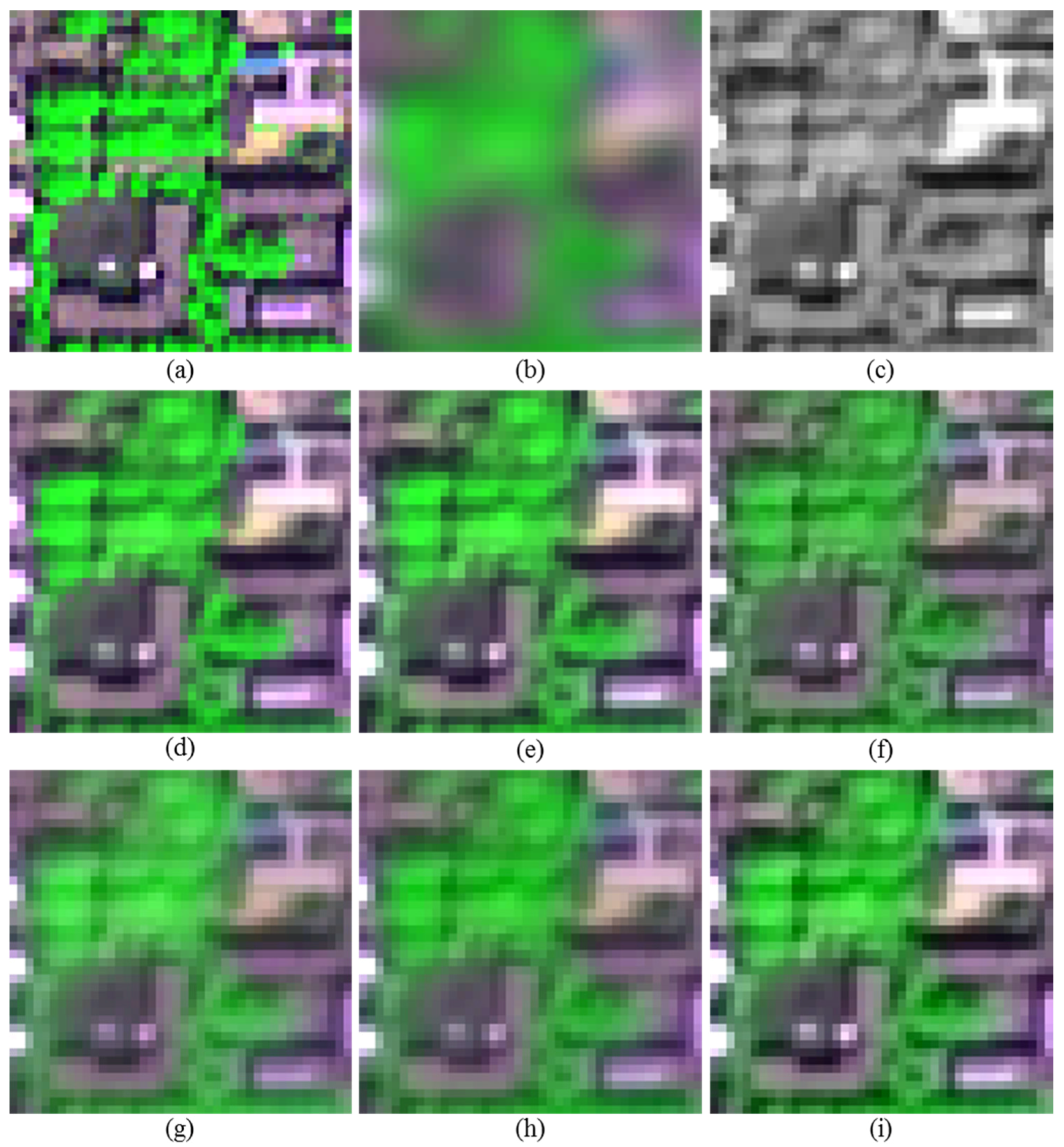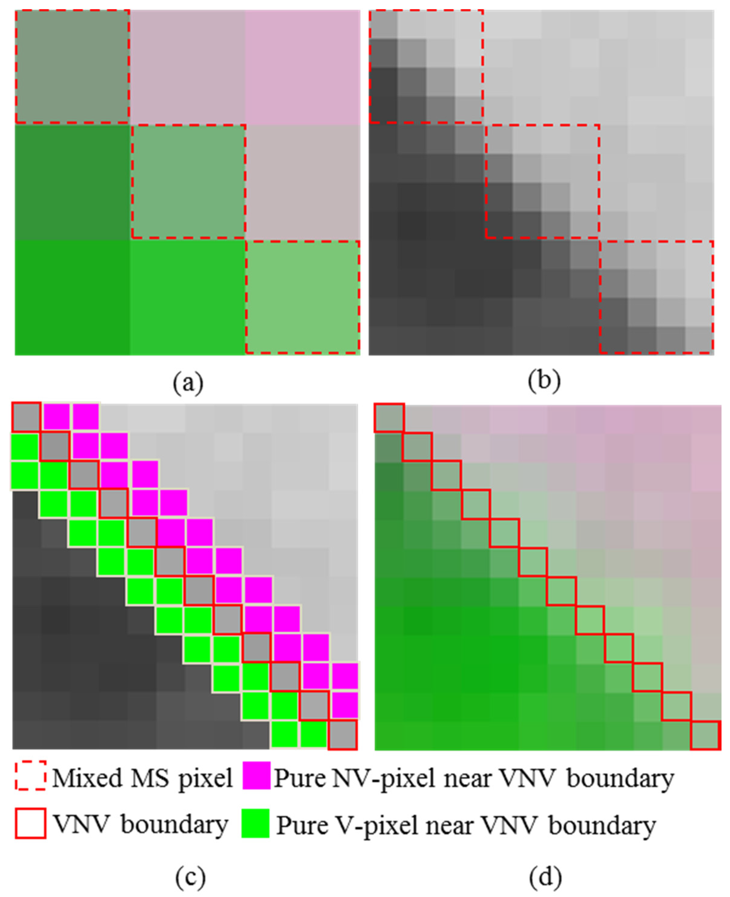Recent studies also demonstrate that an up-sampled MS image generated by current up-sampling methods is not spectrally consistent with the real high spatial resolution MS image at PAN scale for preserving spectral information [38]. However, commonly-used image fusion methods rarely consider the spectral distortions introduced by the up-sampled MS image. Due to the differences in spatial resolution between the MS and PAN images, the up-sampled MS image contains a large number of mixed sub-pixels that correspond to pure pixels in the PAN image. However, the fused versions of these mixed sub-pixels remain mixed in the fusion products generated by current fusion methods. Additionally, these fused pixels are significantly spectrally different from the corresponding real MS pixels of the same spatial resolution of the PAN image. Such mixed fused versions of these mixed sub-pixels bring in blurred boundaries between different objects and significant spectral distortions in the fusion products. As shown in Figure 1, each LSR MS pixel (Figure 1a) covers several PAN pixels (Figure 1b) and also covers several sub-pixels in its up-sampled version at the PAN scale. Some of the sub-pixels of a mixed MS pixel cover mixed PAN pixels (i.e., edge pixels across the boundaries between different objects). The PAN pixels that lie across the boundaries between vegetation and non-vegetation (VNV boundaries) shown in Figure 1c are an example of this. The other sub-pixels of the same mixed MS pixel cover pure PAN pixels near these edge pixels; examples are the pure vegetation (V) and non-vegetation (NV) pixels near VNV boundaries. Typically, the fused versions of all of the sub-pixels of a mixed MS pixel remain mixed in the fused products generated by current fusion methods, although some of them correspond to pure PAN pixels. For example, in the GS-fused image shown in Figure 1d, the fused versions of the mixed sub-pixels that correspond to pure PAN (V and NV) pixels near the VNV boundaries remain mixed. From here on in this paper, the sub-pixels of mixed MS pixels that correspond to pure PAN pixels are referred to as MSPs, whereas the edge pixels that lie across boundaries between different objects are referred to as boundary pixels. It is desirable that these MSPs are set to either pure vegetation pixels or pure non-vegetation pixels in the fused images in order to reduce spectral distortions.

Figure 1. Mixed multispectral (MS) sub-pixels and the corresponding PAN and fused images. (a) The mixed MS pixels at MS resolution; (b) the PAN pixels corresponding to the MS pixels in (a); (c) PAN (edge) pixels across vegetation and non-vegetation (VNV) boundaries and pure PAN (V and NV) pixels near the VNV boundaries; (d) Gram–Schmidt (GS)-fused image overlain with VNV boundaries from the PAN image.

Figure 1. Mixed multispectral (MS) sub-pixels and the corresponding PAN and fused images. (a) The mixed MS pixels at MS resolution; (b) the PAN pixels corresponding to the MS pixels in (a); (c) PAN (edge) pixels across vegetation and non-vegetation (VNV) boundaries and pure PAN (V and NV) pixels near the VNV boundaries; (d) Gram–Schmidt (GS)-fused image overlain with VNV boundaries from the PAN image.

Due to the significant spectral differences between vegetation and non-vegetation objects, the mixed fused versions of the MSPs near the edge pixels lying across VNV boundaries contribute much to the spectral distortions of the fused images. In this paper, an improved image fusion method is proposed to realize the spectral un-mixing of MSPs near VNV boundaries during the fusion process. In this study, the word “un-mixing” means to set the fused version of an MSP into a pure pixel that has the same land cover category (i.e., vegetation or non-vegetation category) as the corresponding PAN pixel. This is significantly different from both the spectral endmember un-mixing technique [39] and the un-mixing-based fused method introduced by Zhukov et al. [40], which is also referred to as the multisensor multiresolution technique (MMT). The former uses pure spectra of different land cover classes (i.e., reference spectra of endmembers) to derive the proportion of each endmember in mixed pixels. The latter is based on the classification of high spatial resolution data, followed by the un-mixing of low spatial resolution MS pixels to retrieve signals of the LSR sensor for the classes recognized in the high spatial resolution data and the reconstruction of high spatial resolution data with the same spectral-resolution as the LSR data. The spectral endmember un-mixing technique is widely used to analyze the mixed pixels in multispectral and hyperspectral images, whereas the MMT is used for the fusion of an LSR MS image with a high spatial resolution multispectral image rather than a monochromatic image (i.e., a PAN band). In this study, the proposed method is used to fuse a high spatial resolution PAN image with an LSR MS image obtained by the same satellite.

In the proposed method in this paper, MSPs near VNV boundaries are identified, and their land cover categories (i.e., vegetation or non-vegetation) are determined. Then, each identified MSP is fused to a vegetation pixel or a non-vegetation pixel using the HR fusion method, depending on the corresponding land cover category. Hence, the identified MSPs near VNV boundaries are spectrally un-mixed to pure vegetation and non-vegetation pixels in the resultant fused image. This improved HR method, which includes the un-mixing of the MSPs, is given the name “UHR”.

This paper is organized as follows. The proposed method is introduced in Section 2, and the experimental results, including visual and quantitative comparisons with other fusion methods, are presented in Section 3. The discussion is presented in Section 4, and Section 5 concludes the paper.

2. Methodologies

Given the registered MS and PAN imagery, MSPs near VNV boundaries are first identified using the coarse VNV boundaries generated from an NDVI (Normalized Difference of Vegetation Index) image derived from the up-sampled MS bands and the fine boundaries (between different objects) generated from the PAN band. A land cover category map for the identified MSPs, which is a prerequisite for the un-mixing of the MSPs, is generated by dividing the identified MSPs into the vegetation and non-vegetation categories based on the categories in the MS and PAN images. Finally, each of the identified MSPs is fused to be either a pure vegetation pixel or a pure non-vegetation pixel, according to the corresponding land cover category. The remaining MS sub-pixels (i.e., the sub-pixels that are not identified as MSPs near VNV boundaries) are fused using the HR method. The details of this process are described in the following sections. The notation used in the next sections is detailed as follows. The high spatial resolution PAN image is denoted as P, the ratio of the spatial resolutions of the MS and PAN images R, the number of spectral bands in the MS image N, the up-sampled MS image $\widetilde{MS}$, the fused MS image $\widehat{MS}$ and the NDVI image derived from the up-sampled MS image I_NDVI.

2.1. Identification of the MSPs near the VNV Boundaries

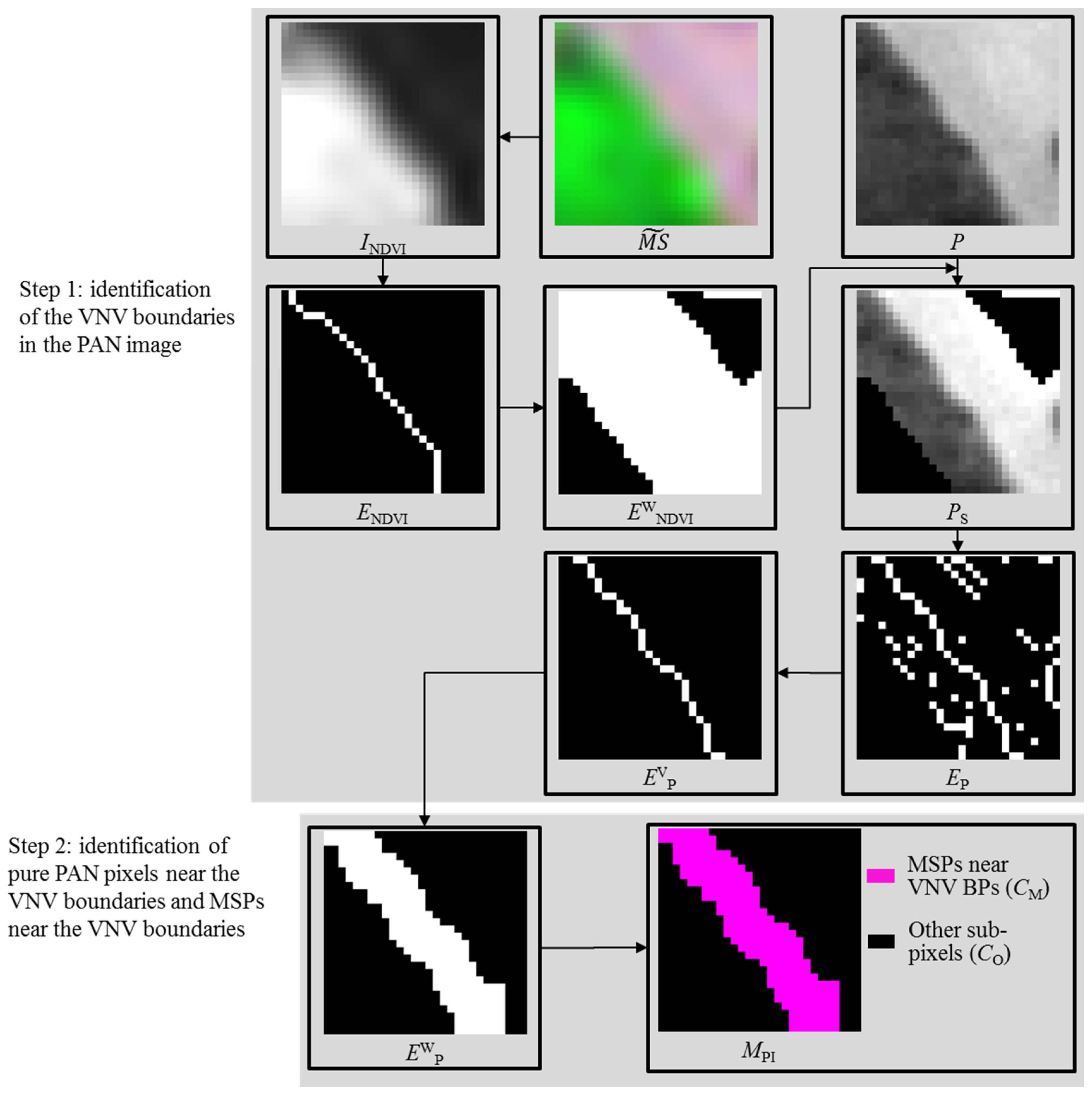
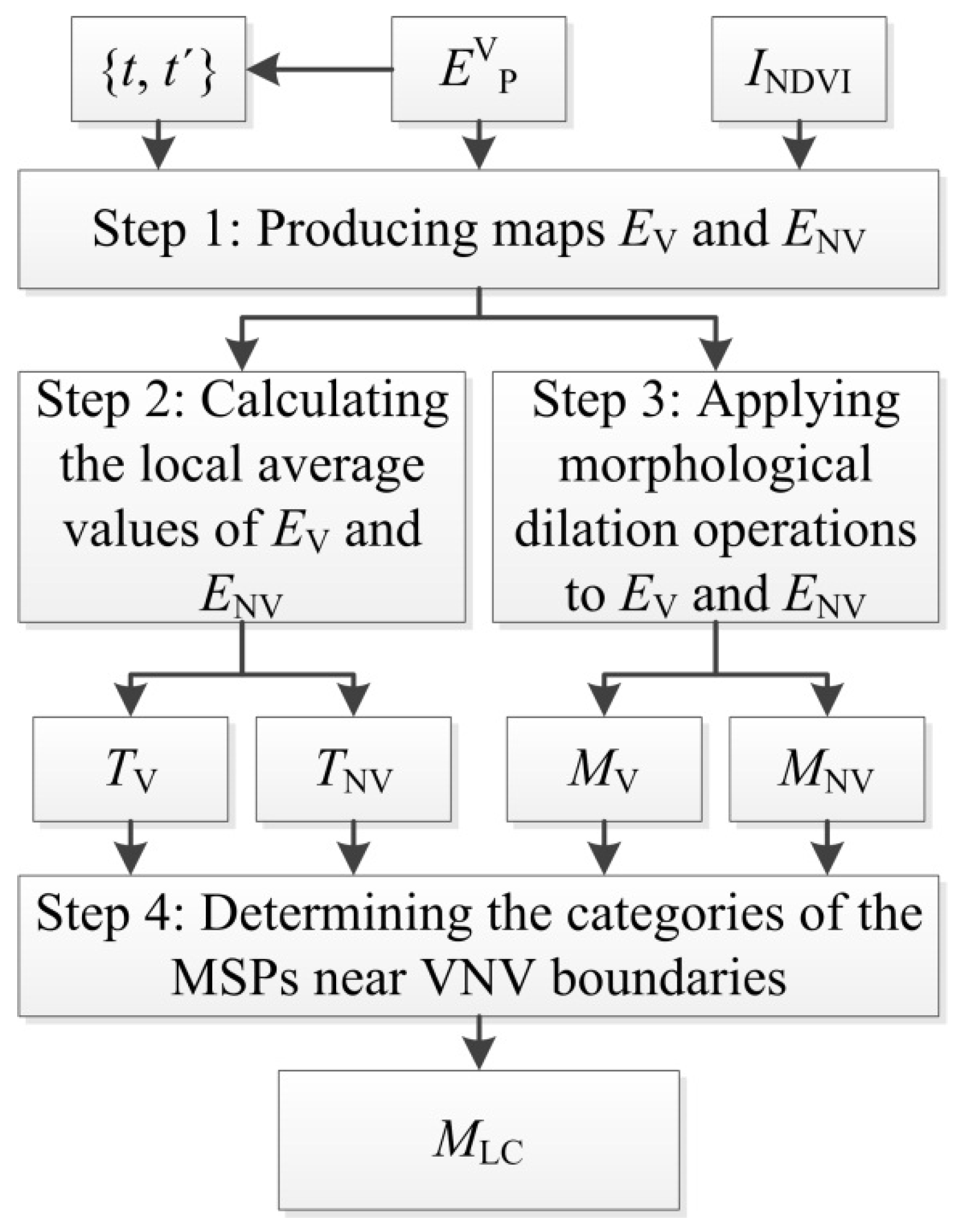
After the up-sampled MS image is produced by up-sampling the MS image to match the pixel size of the PAN image, MSPs near VNV boundaries are identified according to the procedure shown in Figure 2.

Step 1: VNV boundaries in the PAN image are identified using the following steps.

(1)

An edge map, E_NDVI, which includes coarse VNV boundaries from I_NDVI, is produced by applying an Laplacian of Gaussian (LOG) edge detector [41] to a binary image generated from I_NDVI. This binary image has been previously produced by applying a threshold (T_V) obtained using the automatic threshold selection method proposed by Otsu [42]. In the E_NDVI, edge and non-edge pixels have values of 1 (true) and 0 (false), respectively. The edge pixels are then considered to be coarse VNV boundaries generated from I_NDVI.

(2)

Because $\widetilde{MS}$ lacks spatial detail, the VNV boundaries in the PAN image may be displaced relative to the coarse VNV boundaries generated from I_NDVI. To limit the extensions in which VNV boundaries in the PAN image corresponding to the coarse VNV boundaries in I_NDVI are searched for, a mask map, E^W_NDVI, is then generated by applying to the E_NDVI a morphologically-dilated operator using a disk-shaped structure element (SE) with a diameter of L_V.

Next, a subset of the PAN image, PS, is generated by clipping the PAN image using the E^W_NDVI as a mask image. Using PS to find the fine VNV boundaries in the PAN image helps to reduce the amount of calculation. Since the displacements between the VNV boundaries in the PAN image and the corresponding coarse VNV boundaries generated from INDVI are mainly determined by the spatial resolution ratio R, the value of LV can also be set according to R. Since a mixed MS pixel may overlap all of the sub-pixels within a window of size R × R, the displacement between an edge pixel lying across the coarse VNV boundaries and the corresponding edge pixel lying across the fine VNV boundaries in the PAN image is no larger than 2R − 1. Consequently, the value of LV should be no higher than 2R−1 in the case of fine alignment between MS and PAN bands.

(3)

An edge map, E_P, is calculated by applying an LOG edge detector with a standard deviation of δ to P_S. Similar to E_NDVI, the edge and non-edge pixels in E_P have values of 1 (true) and 0 (false), respectively. The value of δ also determines the window size S_G of the LOG detector, i.e., S_G = (δ × 3) × 2 + 1. The LOG detector uses a Gaussian filter specified by δ and S_G to smooth the input image before the edge detection, in order to reduce the effects of noises. A large S_G results in a small number of edge pixels being detected by the LOG algorithm and may lead to incorrect positioning of edge pixels. Hence, the value of δ is set to 0.3, which results in an S_G of 3, in the UHR method.

(4)

To remove edge pixels that do not lie across VNV boundaries in E_P, an edge map E^V_P is generated by setting the value of each pixel t. E^V_P(t) is determined with respect to the values of both E_P(t) and I_NDVI(t), along with the NDVI value of a neighboring pixel $t^{\prime }$, which has the largest difference from pixel t in the PAN image. This is done according to Equation (1):

$$E_P^V(t)\left\{\begin{array}{l}0,\mathrm{if}{E}_{\mathrm{P}}(t)=0\\ 0,\mathrm{if}\max (I_{\mathrm{NDVI}}(t),I_{\mathrm{NDVI}}(t\prime ))<T_{\mathrm{V}}\mathrm{and}{E}_{\mathrm{P}}(t)=1,\\ 0,\mathrm{if}\min (I_{\mathrm{NDVI}}(t),I_{\mathrm{NDVI}}(t\prime ))>T_{\mathrm{V}}\mathrm{and}{E}_{\mathrm{P}}(t)=1\\ 1,\mathrm{otherwise}\end{array}\right\}$$

(1)

where $I_{\mathrm{NDVI}}\left(t\right)$ and $I_{\mathrm{NDVI}}\left(t^{\prime }\right)$ are the NDVI values of pixels t and $t^{\prime }$, respectively, and Tv is a threshold obtained using the OTSU method, as introduced in Subsection 2.1. The purposes of the second and third lines of Formula (1) are to eliminate the boundary pixels that do not lie across VNV boundaries in the PAN image. The two lines are based on a fact that once either pixel t or $t^{\prime }$ lies across VNV boundaries in the PAN image, one of them will have a relative high DNVI value, and the other should have a relative low NDVI value. Once both pixels have high or low DNVI values, they lie in a pure vegetation area or a non-vegetation area and should be eliminated from E_P to yield an edge map E^V_P. In E^V_P, only the edge pixels at the VNV boundaries in the PAN image have values of 1 (true).

Step 2: After the identification of the VNV boundaries in the PAN image, the pixels on both sides of the identified VNV boundaries are identified as MSPs near VNV boundaries, as follows.

(1)

The pixels on both sides of the identified VNV boundaries are identified as pure PAN pixels near VNV boundaries by means of a morphological dilation operation. A morphological dilation operation using a disk-shaped SE with a diameter of L_P is applied to E^V_P to generate a map, E^W_P, in which both the VNV boundaries and the pure PAN pixels near the VNV boundaries have values of 1 (true). The value of L_P determines the maximum distance (in pixels) between the pure PAN pixels near VNV boundaries and the nearest VNV boundaries. For a spatial resolution of R, a pure PAN pixel corresponding to the same mixed MS pixel as a VNV BP pixel, p, will lie within a window with a width of 2R − 1, centered at p. Consequently, the value of L_P can be set to 2R − 1. In practice, the value of L_P may be also affected by the interpolation method employed to yield the up-sampled MS image.

(2)

Mark each sub-pixel t in the up-sampled MS image as an MSP near VNV boundaries only if $E_{\mathrm{P}}^{\mathrm{W}}\left(t\right)=1$. A pixel classification map $M_{\text{PI}}$ is produced by assigning the MSPs near VNV boundaries to category C_M and all others to category C_O, according to Equation (2):

$$M_{\text{PI}}\left(t\right)=\{\begin{array}{cc}{C}_{\mathrm{M}},& E_{\mathrm{P}}^{\mathrm{W}}\left(t\right)=1\\ C_{\mathrm{O}},& E_{\mathrm{P}}^{\mathrm{W}}\left(t\right)=0\end{array}$$

(2)

The MSPs belonging to the category C_M in $M_{\text{PI}}$ will be un-mixed during the fusion process. Two of the three involved parameters, the diameters of the two disk-shaped SEs (L_V and L_P), are required in this step.

Figure 2. Scheme for the identification of MS sub-pixels (MSPs) near VNV boundaries.

Figure 2. Scheme for the identification of MS sub-pixels (MSPs) near VNV boundaries.

2.2. Determining the Categories of the Identified MSPs

In order to set the fused version of the MSPs near VNV boundaries (i.e., the sub-pixels with category C_M) as pure vegetation or non-vegetation pixels, the land cover categories (i.e., vegetation or non-vegetation) of the MSPs should be determined first and act as a prerequisite for the un-mixing during the fusion process.

The NDVI can be employed to divide a pixel into the vegetation and non-vegetation categories since a vegetation pixel usually has a higher NDVI than a non-vegetation one. However, MSPs near the VNV boundaries may also have high NDVI values due to the high NDVI values of the corresponding mixed MS pixels, which consist of combinations of vegetation and non-vegetation objects. Consequently, it is difficult to divide the identified MSPs into the vegetation and non-vegetation categories by applying a single threshold to the whole NDVI image. Hence, two maps, T_V and T_NV, which record the local average NDVI values of vegetation edge pixels and non-vegetation edge pixels, respectively, are produced, and the category of each identified MSP is then determined with respect to the corresponding values recorded in the two maps.

Moreover, ideally, vegetation pixels will lie on one side of the VNV boundaries and the non-vegetation pixels on the other side. Hence, a vegetation pixel map, M_V, and a non-vegetation pixel map, M_NV, are generated by applying morphological dilation operations to the vegetation edge pixels map, E_V, and the non-vegetation edge pixels map, E_NV. Finally, M_V, M_NV, T_V and T_V, along with the NDVI, are used to determine the land cover category (i.e., vegetation or non-vegetation) of each identified MSP. The flow diagram for the classification of the identified MSPs is shown in Figure 3, and the details of each step of this procedure are listed below.

Figure 3. The flow diagram of the classification of the MSPs near VNV boundaries.

Figure 3. The flow diagram of the classification of the MSPs near VNV boundaries.

Step 1: A vegetation edge pixels map E_V and a non-vegetation edge pixels map E_NV are generated with respect to E^V_P in this step. All of the pixels that are true in E_V are the vegetation pixels that lie across VNV boundaries, whereas all of the pixels that are true in E_NV are the non-vegetation pixels that lie across VNV-boundaries. The details of this step are introduced as follows:

(1)

For each pixel, t, that is true in E^V_P (i.e., E^V_P(t) = 1), a neighboring pixel, $t^{\prime }$, with the largest spectral difference from the pixel t, is searched for in the eight-pixel neighborhood of t. This results in a list of pixel pairs, {t,$t^{\prime }$};

(2)

Based on the pixel pairs {t,$t^{\prime }$} and the NDVI, the vegetation edge pixels map, E_V, and the non-vegetation edge pixels map, E_V, are produced according to Equation (3):

$$\begin{array}{c}{E}_{\mathrm{V}}\left(t^{\mathrm{V}}\right)=1,E_{\mathrm{V}}\left(t^{\mathrm{NV}}\right)=0\\ E_{\mathrm{NV}}\left(t^{\mathrm{NV}}\right)=1,E_{\mathrm{NV}}\left(t^{\mathrm{V}}\right)=0\end{array}$$

(3)

where $t^{\mathrm{V}}$ and $t^{\mathrm{NV}}$ are determined using Equation (4).

$$\begin{array}{c}{t}^{\mathrm{V}}=t,t^{\mathrm{NV}}=t^{\prime },\text{ if }{I}_{\mathrm{NDVI}}\left(t\right)>I_{\mathrm{NDVI}}\left(t^{\prime }\right)\\ t^{\mathrm{V}}=t^{\prime },t^{\mathrm{NV}}=t,\text{ if }{I}_{\mathrm{NDVI}}\left(t\right)<I_{\mathrm{NDVI}}\left(t^{\prime }\right)\end{array}$$

(4)

The maps E_V and E_NV are employed to generate the maps T_V and T_NV in the next step.

Step 2: The maps T_V and T_NV, which record the local average NDVI values of vegetation edge pixels and non-vegetation edge pixels, respectively, are produced in this step. The maps are generated by assigning the value of each pixel, p, in the two maps, according to Equations (5) and (6), respectively:

$$T_{\mathrm{V}}\left(p\right)=\frac{{{\displaystyle \sum }}_{j\in N_{S_{\mathrm{p}}}\left(p\right)}\left(I_{\mathrm{NDVI}}\left(j\right)\times E_{\mathrm{V}}\left(j\right)\right)}{{{\displaystyle \sum }}_{j\in N_{S_{\mathrm{p}}}\left(p\right)}{E}_{\mathrm{V}}\left(j\right)}$$

(5)

$$T_{\mathrm{NV}}\left(p\right)=\frac{{{\displaystyle \sum }}_{j\in N_{S_{\mathrm{p}}}\left(p\right)}\left(I_{\mathrm{NDVI}}\left(j\right)\times E_{\mathrm{NV}}\left(j\right)\right)}{{{\displaystyle \sum }}_{j\in N_{S_{\mathrm{p}}}\left(p\right)}{E}_{\mathrm{NV}}\left(j\right)}$$

(6)

where $N_{S_{\mathrm{P}}}\left(p\right)$ is a neighboring window with a size of S_P × S_P pixels of pixel p. Since a high value of S_P will increase the amount of calculation, S_P can be set equal to 2R − 1.

Step 3: The maps M_V and M_NV are generated by iteratively applying morphological dilation operations to E_V and E_NV as follows.

(1)

The vegetation map, M_V, is produced by applying a morphological dilation operator using a disk-shaped SE with a diameter of 3 pixels to E_V. The pixels that are true in M_V and also true in E_NV are then set to be false in M_V.

(2)

The resultant vegetation map, M_V, in which the pixels that are true represent vegetation, is obtained by iterating Step 1 R − 1 times.

(3)

The non-vegetation map, M_NV, is generated by applying the morphological dilation operator described in Step 1 to E_NV. The pixels that are true in M_NV and also in E_V are then set to be false in M_NV.

(4)

The resultant non-vegetation map, M_NV, in which the pixels that are true represent non-vegetation, is obtained by iterating Step 3 R − 1 times.

Step 4: The category (i.e., vegetation or non-vegetation) of each of the identified MSPs (denoted as pixel m) is determined, according to Equation (7):

$$M_{\mathrm{LC}}\left(m\right)=\{\begin{array}{cc}{C}_{\mathrm{V}},& \text{if }{M}_{\mathrm{V}}\left(m\right)=1and(M_{\mathrm{NV}}\left(m\right)=0or{I}_{\mathrm{NDVI}}\left(m\right)>T_{\mathrm{V}}\left(m\right))\\ C_{\mathrm{NV}},& \text{if }{M}_{\mathrm{NV}}\left(m\right)=1and(M_{\mathrm{V}}\left(m\right)=0or{I}_{\mathrm{NDVI}}\left(m\right)<T_{\mathrm{NV}}\left(m\right))\end{array}$$

(7)

An MSP m that is true in $M_{\mathrm{V}}\left(m\right)$ is determined to be a vegetation pixel if $M_{\mathrm{NV}}\left(m\right)=0$ or $I_{\mathrm{NDVI}}\left(m\right)>T_{\mathrm{V}}\left(m\right)$, whereas an MSP, m, that is true in $M_{\mathrm{NV}}\left(m\right)$ is determined to be a non-vegetation pixel if $M_{\mathrm{V}}\left(m\right)=0$ or $I_{\mathrm{NDVI}}\left(m\right)<T_{\mathrm{NV}}\left(m\right)$. Eventually, all of the identified MSPs will be divided into the vegetation and non-vegetation categories, and a classification map, $M_{\mathrm{LC}}$, is produced to assist the fusion of the identified MSPs.

The size of the neighboring window, S_P, is the only parameter that needs to be decided upon in the classification.

2.3. Fusion of the MS Sub-Pixels

The HR fusion method is employed to yield the fused versions of the MS sub-pixels in the proposed method, for its better performances than other methods [21], such as the SVR, GS and PS methods. In order to reduce spectral distortions, the fused version of each identified MSP (i.e., the sub-pixels with category $C_{\mathrm{M}}$ in M_PI) is calculated with reference to the spectra of a neighboring pure (vegetation or non-vegetation) pixel. The fused versions of the sub-pixels with category $C_{\mathrm{O}}$ in M_PI are calculated with reference to their own spectra.

The HR method is a PAN modulation fusion method that takes haze into account [43,44,45]. In this method, the fused i-th spectral band of pixel t, ${\widehat{MS}}_i\left(t\right)$, is calculated by using Equation (8):

$${\widehat{MS}}_i\left(t\right)=\left({\widetilde{MS}}_i\left(t\right)-H_i\right)\frac{P\left(t\right)-H_{\mathrm{p}}}{P_{\mathrm{L}}\left(t\right)-H_{\mathrm{p}}}+H_i$$

(8)

where P_L is a low-pass filtered version of P; ${\widetilde{MS}}_i$ and ${\widehat{MS}}_i$ are the i-th bands of the up-sampled and fused MS images, respectively; and H_i and H_p denote the haze values in the i-th MS band and PAN band, respectively. The H_i and H_p can be determined using the minimum grey level values in the i-th MS band and P_L according to an image-based dark-object subtraction method [43,44,45]. The HR method uses the spectral distortion minimizing (SDM) model [46] as the injection model and clumps the spectral angles between the fused and up-sampled MS pixels. It can be proven that the spectra vector of pixel t in the fused image (${\widehat{\mathit{V}}}_t=\left\{{\widehat{MS}}_1\left(t\right),{\widehat{MS}}_2\left(t\right),\dots ,{\widehat{MS}}_N\left(t\right)\right\}$) is parallel to that of t in the up-sampled image (${\tilde{\mathit{V}}}_t=\left\{{\widetilde{MS}}_1\left(t\right),{\widetilde{MS}}_2\left(t\right),\dots ,{\widetilde{MS}}_N\left(t\right)\right\}$) [46].

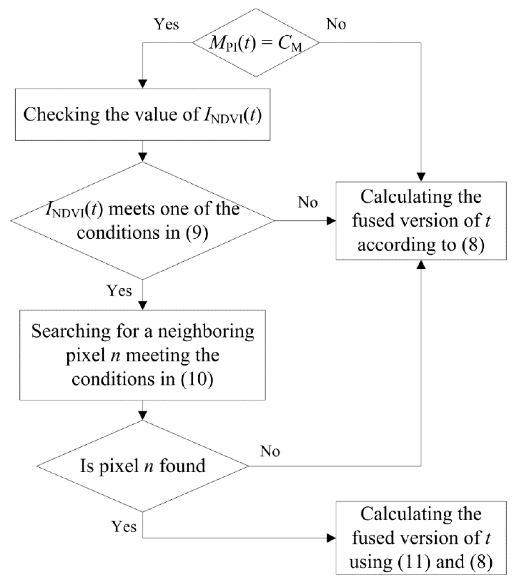
As the flow diagram shown in Figure 4, each MS sub-pixel is fused according to the appropriate category (i.e., either the identified MSPs or the remaining sub-pixels) in M_PI.

Figure 4. The flow diagram for the fusion of the MS sub-pixels.

Figure 4. The flow diagram for the fusion of the MS sub-pixels.

(1)

For a sub-pixel, t,if $M_{\text{PI}}\left(t\right)=C_{\mathrm{O}}$, its fused version is calculated according to Equation (8). Otherwise, its land cover category, $M_{\mathrm{LC}}\left(t\right)$, is examined with respect to the value of $I_{\mathrm{NDVI}}\left(t\right)$, according to the two conditions in Equation (9).

$$\{\begin{array}{c}{I}_{\mathrm{NDVI}}\left(t\right)\ge \frac{{{\displaystyle \sum }}_{j\in N_{S_{\mathrm{N}}}\left(t\right)}\left(I_{\mathrm{NDVI}}\left(j\right)\times E_{\mathrm{V}}\left(j\right)\right)}{{{\displaystyle \sum }}_{j\in N_{S_{\mathrm{N}}}\left(t\right)}{E}_{\mathrm{V}}\left(j\right)},\text{ if }{M}_{\mathrm{LC}}\left(t\right)=C_{\mathrm{V}}\\ I_{\mathrm{NDVI}}\left(t\right)\le \frac{{{\displaystyle \sum }}_{j\in N_{S_{\mathrm{N}}}\left(t\right)}\left(I_{\mathrm{NDVI}}\left(j\right)\times E_{\mathrm{NV}}\left(j\right)\right)}{{{\displaystyle \sum }}_{j\in N_{S_{\mathrm{N}}}\left(t\right)}{E}_{\mathrm{NV}}\left(j\right)},\text{ if }{M}_{\mathrm{LC}}\left(t\right)=C_{\mathrm{NV}}\end{array},$$

(9)

where $N_{S_{\mathrm{N}}}\left(t\right)$ is a window with a size of S_N × S_N pixels centered at pixel t, and E_V and E_NV are the vegetation edge pixels map and the non-vegetation edge pixels map, respectively, as introduced in Section 2.2. The first condition is based on the fact that if $M_{\mathrm{LC}}\left(t\right)=C_{\mathrm{V}}$, $I_{\mathrm{NDVI}}\left(t\right)$ should be higher than the average NDVI value of the surrounding vegetation edge pixels in E_V. The second condition is based on the fact that if $M_{\mathrm{LC}}\left(t\right)=C_{\mathrm{NV}}$, $I_{\mathrm{NDVI}}\left(t\right)$ should be lower than the average NDVI value of the surrounding non-vegetation edge pixels in E_NV.

(2)

If $I_{\mathrm{NDVI}}\left(t\right)$ meets no conditions in Equation (9), pixel t may be misclassified in $M_{\mathrm{LC}}$, and its fused version is calculated using Equation (8), in order to avoid spectral distortions caused by the incorrect substitutions employed. Otherwise, a neighboring pixel n is searched for among the pixels with the same land cover class as pixel t (i.e., M_LC(t) = M_LC(n)) in a neighboring window $N_{S_{\mathrm{N}}}\left(t\right)$ according to the conditions in Equation (10):

$$\{\begin{array}{c}{I}_{\mathrm{NDVI}}\left(n\right)=\underset{j\in N_{S_{\mathrm{N}}}\left(t\right)\&M_{\mathrm{LC}}\left(j\right)=C_{\mathrm{V}}}{\max }{I}_{\mathrm{NDVI}}\left(j\right)\text{ and }{I}_{\mathrm{NDVI}}\left(n\right)>I_{\mathrm{NDVI}}\left(t\right),\text{ if }{M}_{\mathrm{LC}}\left(t\right)=C_{\mathrm{V}}\\ I_{\mathrm{NDVI}}\left(n\right)=\underset{j\in N_{S_{\mathrm{N}}}\left(t\right)\&M_{\mathrm{LC}}\left(j\right)=C_{\mathrm{NV}}}{\min }{I}_{\mathrm{NDVI}}\left(j\right)\text{ and }{I}_{\mathrm{NDVI}}\left(n\right)<I_{\mathrm{NDVI}}\left(t\right),\text{ if }{M}_{\mathrm{LC}}\left(t\right)=C_{\mathrm{NV}}\end{array}.$$

(10)

The purpose of this step is to find a substitution pixel n for t, depending on $M_{\mathrm{LC}}\left(t\right)$. If t is a vegetation pixel in M_LC (i.e., $M_{\mathrm{LC}}\left(t\right)=C_{\mathrm{V}}$), the sub-pixel n should have the maximum NDVI value in window $N_{S_{\mathrm{N}}}\left(t\right)$ and belong to the same category as t in M_LC (i.e., $M_{\mathrm{LC}}\left(n\right)=M_{\mathrm{LC}}\left(t\right)=C_{\mathrm{V}}$). Otherwise, if t is a non-vegetation pixel in M_LC (i.e., $M_{\mathrm{LC}}\left(t\right)=C_{\mathrm{NV}}$), the sub-pixel n should have the minimum NDVI value in the window $N_{S_{\mathrm{N}}}\left(t\right)$ and belongs to the same category as t (i.e., $M_{\mathrm{LC}}\left(n\right)=M_{\mathrm{LC}}\left(t\right)=C_{\mathrm{NV}}$). The spectra of pixel n will be used to set the fused version of pixel t as a pure vegetation or non-vegetation pixel. In order to avoid spectral distortions introduced by incorrect substitutions used in the fusion, the substitute pixel n is restricted to have an NDVI value higher than that of t if $M_{\mathrm{LC}}\left(t\right)=C_{\mathrm{V}}$, whereas it is restricted to have an NDVI value lower than that of t if $M_{\mathrm{LC}}\left(t\right)=C_{\mathrm{NV}}$.

(3)

If no such pixel n meets the conditions in Equation (10), the fused version of $t$ is calculated using Equation (8). Otherwise, ${\widetilde{MS}}_i\left(n\right)$ and $P_{\mathrm{L}}\left(n\right)$, the spectral values of the pixel n in ${\widetilde{\text{MS}}}_i$ and P_L, are assigned to ${\widetilde{MS}}_i\left(t\right)$ and $P_{\mathrm{L}}\left(t\right)$, respectively, as Equation (10), and then, the fused version of t is calculated using Equations (8) and (11).

$$\{\begin{array}{c}{\widetilde{MS}}_i\left(t\right)={\widetilde{MS}}_i\left(n\right)\\ P_{\mathrm{L}}\left(t\right)=P_{\mathrm{L}}\left(n\right)\end{array}$$

(11)

In this case, the pixel vector of pixel t in the fused image is parallel to that of the up-sampled pixel n, according to the SDM injection model employed in the HR method. It is assumed that pixel n is a pure vegetation or non-vegetation pixel, and therefore, MSP t is fused to be a pure vegetation or non-vegetation pixel in the resultant fused image, realizing spectral un-mixing in the fusion process and reducing the spectral distortion in the fused product.

In this step, parameter S_N stands for the size of the neighborhood window within which to search for a substitution pixel used to un-mix an MSP in the fusion process. The parameter is mainly determined by the spatial resolution ratio R, along with the interpolation method employed to generate the up-sampled MS. Specifically, a pure PAN pixel corresponding to the same mixed MS pixel as t lies within a window with a width of 2R−1 centered at t. Consequently, the value of S_N can be set to 2R − 1, or slightly lower than 2R−1, in order to avoid over-un-mixing.

3. Experiments

3.1. Test Data, Fusion Methods for Comparison and Evaluation Criteria

Two datasets acquired by the WorldView-2 (WV-2) and the IKONOS sensors were used to assess the performance of the proposed method. The WV-2 sensor provides data in eight MS bands and a PAN band with 2-m and 0.5-m spatial resolutions, respectively. The MS bands include four conventional visible and near-infrared MS bands: blue (B, 450–510 nm), green (G, 510–580 nm), red (R, 630–690 nm) and near-IR1 (NIR1, 770–895 nm); and four new bands: coastal (C, 400–450 nm), yellow (Y, 585–625 nm), red edge (RE, 705–745 nm) and near-IR2 (NIR2, 860–1040 nm). The WV-2 PAN band, for which the spectral response range is 450–800 nm, covers a narrower NIR spectral range than the IKONOS PAN band. The WV-2 dataset was acquired in September 2014 over the city of Beijing, China, and had an average off-nadir angle of 13.7°. The IKONOS sensor provides data in four MS bands with 4-m spatial resolution. These comprise the blue (B, 0.45–0.53 μm), green (G, 0.52–0.61 μm), red (R, 0.64–0.72 μm) and near-infrared (NIR, 0.77–0.88 μm) bands, and there is also a corresponding 1-m PAN band (0.45–0.90 μm). The IKONOS dataset was acquired over Beijing in May 2000. These two sensors were chosen for this work, since the two PAN bands have different spectral response ranges. Both of the original MS images from the two sensors had a size of 512 × 512 pixels, and both of the original PAN images had a size of 2048 × 2048 pixels. Typical land cover types in the two scenes included water bodies, grasses, trees, buildings, roads and shadows.

To verify the performance of the proposed fusion scheme, the fused images obtained using the proposed method were compared to methods from the literature that were both well known and known to perform well. These included the HR [21], PS [19,20], GS [12] with Mode 1 (GS1), GS with Mode 2 (GS2) and GS adaptive (GSA) [13] methods.

Two quantitative assessment procedures were adopted to evaluate the performance of the proposed fusion method, along with a visual comparison. The first procedure compared the fused imagery generated from the degraded MS and PAN images of the two sensors with the corresponding original MS images according to Wald’s protocol [47]. Three comprehensive indices, the Erreur Relative Globale Adimensionnell de Synthèse (ERGAS) [48], the Spectral Angle Mapper (SAM) [49,50] and Q2ⁿ [51,52], which is a generalization of the Universal Image Quality Index (UIQI) for monoband images and derived from the theory of hypercomplex numbers, particularly of 2ⁿ-ones, were employed to do this. These indices estimate the global spectral quality of the fused images. The lower the ERGAS and the SAM values, the better the quality of the fused image. The higher the Q2ⁿ index, the better the quality of the fused product. Given the number of bands in the two datasets, the Q4 and Q8 indices were used for the IKONOS and WV-2 datasets, respectively. The second procedure compared the fused versions of the original MS and PAN images of the two sensors using the Quality index with no reference images (QNR) [53]. The QNR is formed from the product of two variables, D_λ and D_S, which quantify the spectral and spatial distortions, respectively. D_λ is derived from the difference between the inter-band UIQI [54] values calculated from the fused MS bands and those calculated from the LSR MS bands. D_S is generated from the difference between the UIQI values calculated using the PAN band and each of the fused MS bands and those calculated using the degraded PAN band and each of the LSR MS bands. The higher the QNR index, the better the quality of the fused product. The maximum theoretical value of the QNR is 1, which occurs when both D_λ and D_S are equal to 0.

3.2. Generation of the Fusion Products for Comparisons

The degraded versions of the WV-2 and IKONOS images were obtained by applying a low-pass filter that matched the modulation transfer function (MTF) of the corresponding sensor and a decimation characterized by a sampling factor equal to the resolution ratio, R, to each band. The fusion experiments were then carried out on both the degraded and original versions of the two datasets.

The PS-fused images were generated in PCI Geomatics software, whereas the other fusion products were produced by using the corresponding algorithms developed in MATLB R2011b (Version 7.13.0.564). For all of the fusion methods, except PS, the up-sampled MS images were generated by using a polynomial kernel with 23 coefficients [55]. For GS2 (GS with Mode 2), GSA, HR and the proposed UHR methods, the low-pass version PAN images (P_L) were produced by employing low-pass filters that matched the MTF of the corresponding sensors [46,56]. The HR-fused images were produced by using the same haze values as for the UHR method. For the UHR method, the NDVI images of the original and degraded WV-2 datasets were obtained by using the bands R and NIR1, whereas those of the original and degraded IKONOS datasets were generated by using the bands R and NIR.

The values of the parameters required by the proposed method were determined according to the explanation given in Section 2. Parameter δ was set to 0.3; the values of S_P, L_V and L_P were set to 7 (2R − 1), 5 (2R − 3) and 7 (2R − 1), respectively, for a value of 4 for R. In addition, the value of S_N is also mainly determined by the spatial resolution ratio, R. The value of S_N can be set to 2R − 1, or slightly lower than 2R − 1 in order to avoid over-un-mixing. The S_N values for the original and degraded datasets were thus set to 7 and 5, respectively, for both the WV-2 and IKONOS datasets.

Finally, the UHR-fused images of the original and degraded WV-2 datasets were produced with 652,048 and 61,901 un-mixed MSPs, respectively. The UHR-fused images of the original and degraded IKONOS datasets were generated with 864,400 and 60,953 un-mixed MSPs, respectively.

3.3. Wald’s Protocol

The quality indices for the fused images produced from the WV-2 and IKONOS datasets at the degraded scale are shown in Table 1. “EXP” in the table refers to interpolated MS images at the PAN scale formed without the injection of details derived from the corresponding PAN bands. 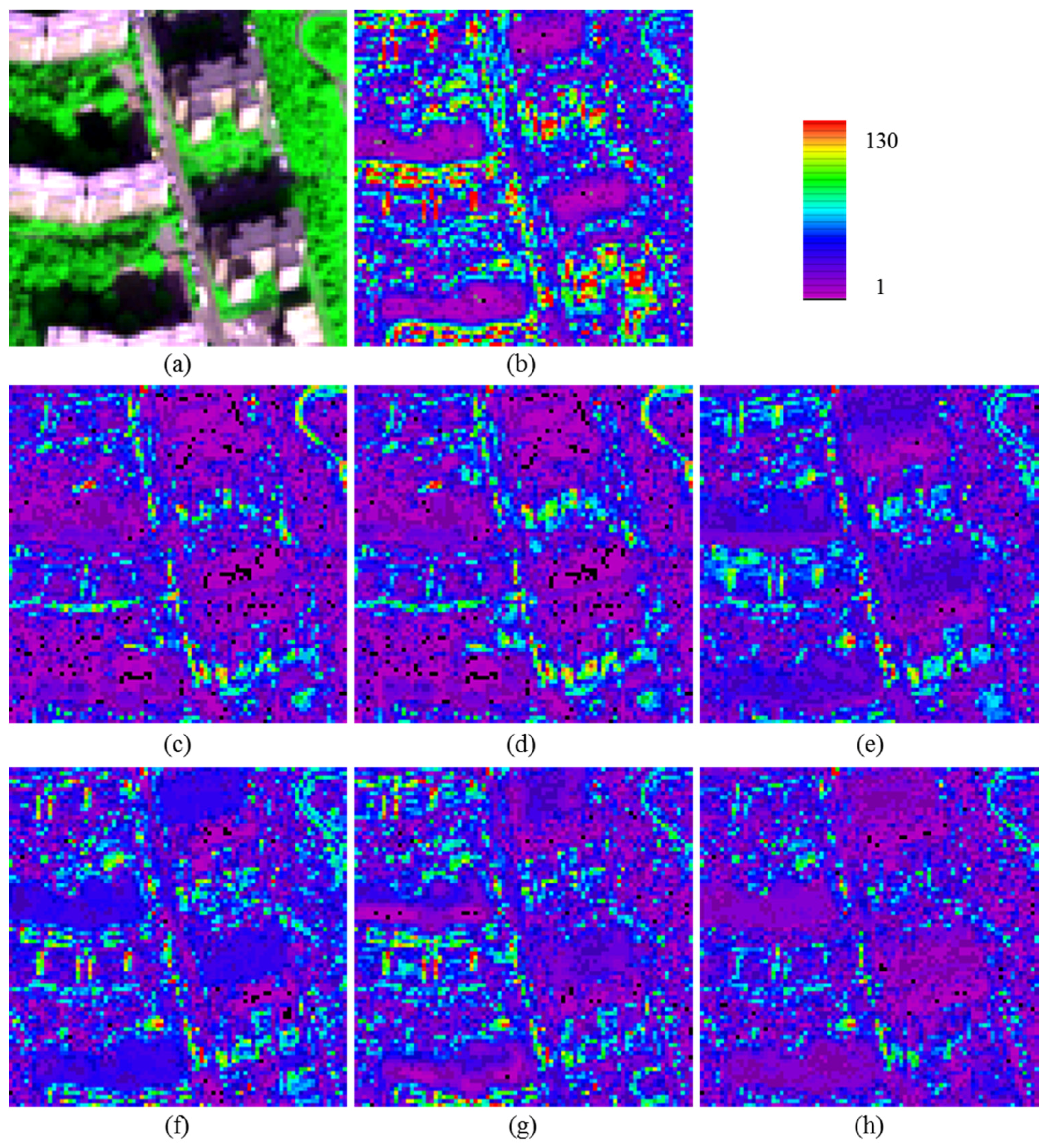In order to observe the fusion products in detail, the subsets of the MS image and the corresponding fused images produced from the degraded WV-2 dataset are shown in Figure 5. In addition, the error maps of the fusion products shown in Figure 5 are shown in Figure 6 to better compare the quality of the fused images. These error maps, which record the root mean square error (RMSE) values of the fused pixels in each of the fusion products, are applied to an identical histogram stretching scheme generated from the error map of the up-sampled MS image. 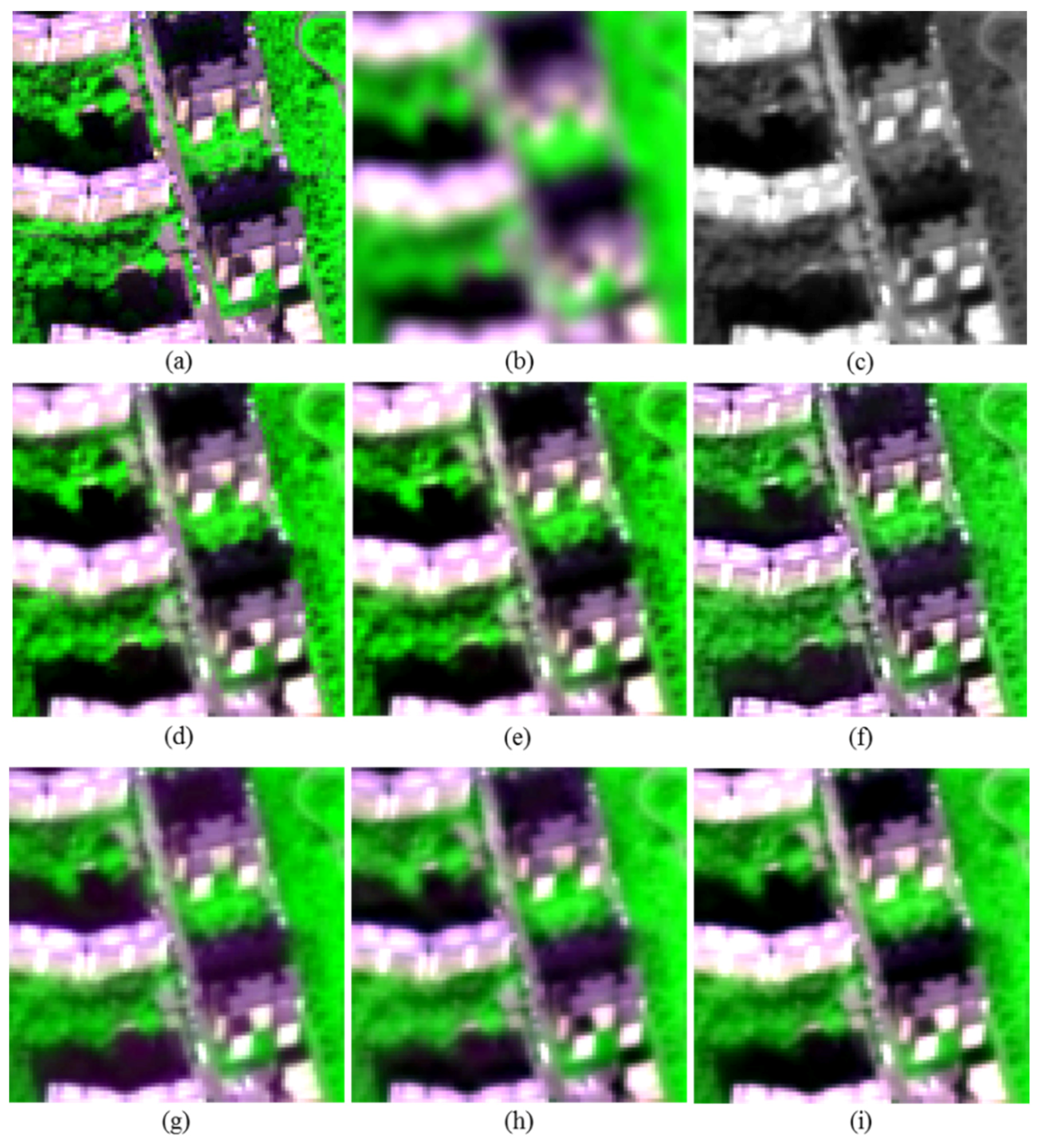The subsets of the MS image and the corresponding fused images produced from the degraded IKONOS dataset are shown in Figure 7. In this study, the original and fused MS images of the WV-2 dataset are shown as a combination of bands R, NIR1 and B, whereas the original and fused MS images of the IKONOS dataset are shown as a combination of bands R, NIR and B. An identical histogram stretching scheme generated from the up-sampled MS image (in the case of the original scale) or the reference MS image (in the case of the degraded scale) was applied to the MS images shown in these two figures.

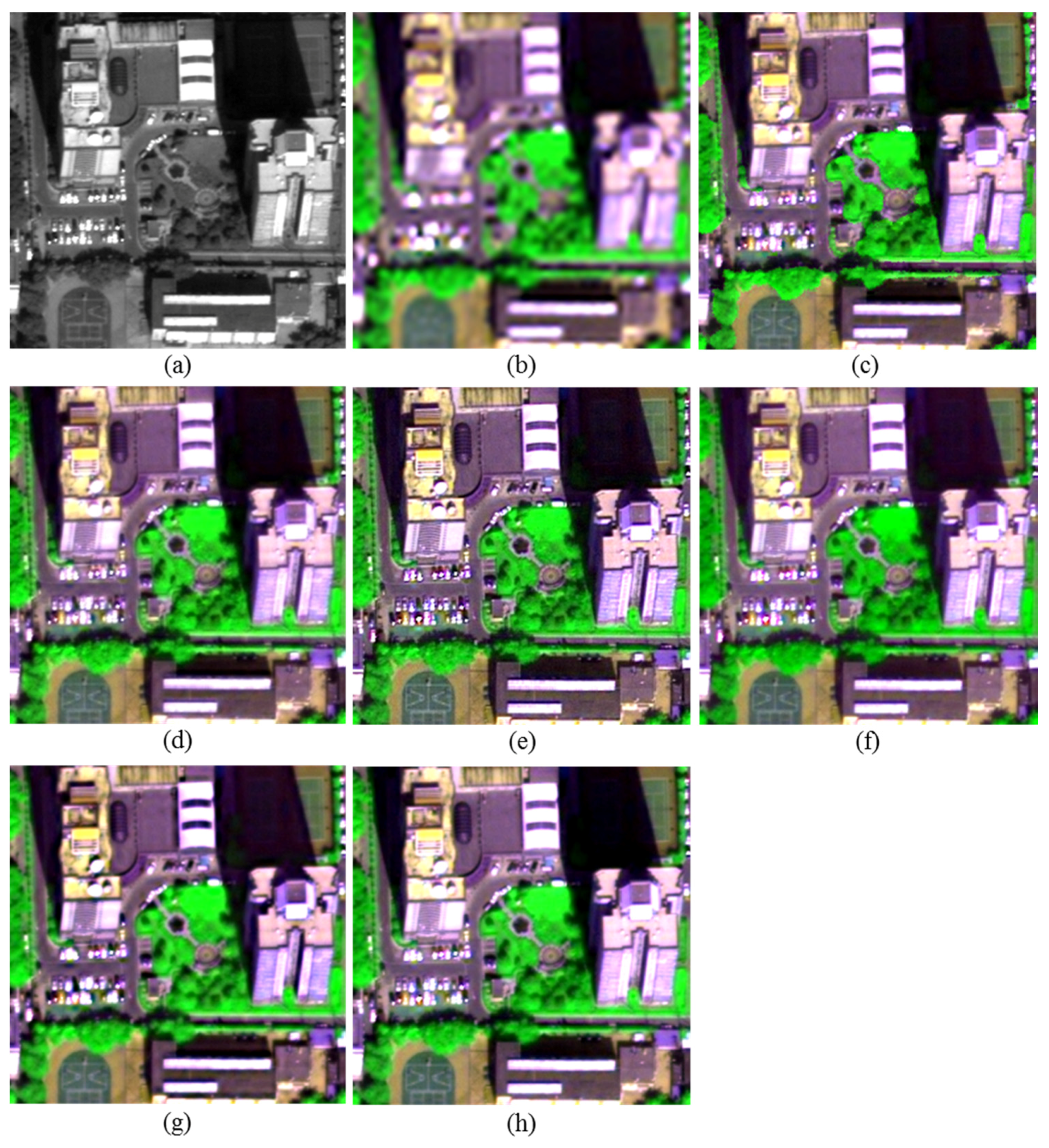
Figure 5. The 84 × 84 pixel subsets of the MS images and the corresponding fused images produced from the degraded WorldView (WV)-2 dataset: (a) true 2-m MS image; (b) up-sampled version of the 8-m MS image; (c) 4-m PAN image; and the results of (d) UHR fusion, (e) HR fusion, (f) PS fusion, (g) GS1 fusion, (h) GS2 fusion and (i) GSA fusion.

Figure 5. The 84 × 84 pixel subsets of the MS images and the corresponding fused images produced from the degraded WorldView (WV)-2 dataset: (a) true 2-m MS image; (b) up-sampled version of the 8-m MS image; (c) 4-m PAN image; and the results of (d) UHR fusion, (e) HR fusion, (f) PS fusion, (g) GS1 fusion, (h) GS2 fusion and (i) GSA fusion.

Table 1. Values of the comprehensive quality indices of the fused images produced from the degraded WV-2 and IKONOS datasets. Q, Quality; UHR, un-mixed haze- and ratio-based (HR); PS, PANSHARP.

	WV-2			IKONOS
	ERGAS	SAM (°)	Q8	ERGAS	SAM (°)	Q4
UHR	2.459	3.052	0.914	1.577	1.882	0.871
HR	2.496	3.197	0.912	1.581	1.931	0.869
PS	2.651	3.752	0.885	1.962	2.403	0.779
GS1	2.997	3.749	0.846	2.112	2.358	0.751
GS2	2.834	3.613	0.865	2.058	2.315	0.760
GSA	2.473	3.440	0.911	1.652	2.067	0.859
EXP	3.826	3.932	0.722	2.673	2.576	0.584

Table 1. Values of the comprehensive quality indices of the fused images produced from the degraded WV-2 and IKONOS datasets. Q, Quality; UHR, un-mixed haze- and ratio-based (HR); PS, PANSHARP.

	WV-2			IKONOS
	ERGAS	SAM (°)	Q8	ERGAS	SAM (°)	Q4
UHR	2.459	3.052	0.914	1.577	1.882	0.871
HR	2.496	3.197	0.912	1.581	1.931	0.869
PS	2.651	3.752	0.885	1.962	2.403	0.779
GS1	2.997	3.749	0.846	2.112	2.358	0.751
GS2	2.834	3.613	0.865	2.058	2.315	0.760
GSA	2.473	3.440	0.911	1.652	2.067	0.859
EXP	3.826	3.932	0.722	2.673	2.576	0.584

Figure 6. The 84 × 84 pixel subsets of the original images and the error maps of the fused images produced from the degraded WV-2 dataset: (a) true 2-m MS image; and the error maps for the results of (b) the up-sampled version of the 8-m MS image; (c) UHR fusion; (d) HR fusion; (e) PS fusion, (f) GS1 fusion; (g) GS2 fusion and (h) GSA fusion.

Figure 6. The 84 × 84 pixel subsets of the original images and the error maps of the fused images produced from the degraded WV-2 dataset: (a) true 2-m MS image; and the error maps for the results of (b) the up-sampled version of the 8-m MS image; (c) UHR fusion; (d) HR fusion; (e) PS fusion, (f) GS1 fusion; (g) GS2 fusion and (h) GSA fusion.

Comparison between the fusion products (of the two sensors) generated by the six approaches shows that the proposed UHR method provides the best result in terms of ERGAS, SAM and Q8, followed by the HR and GSA methods. The GSA and PS perform better than the GS2 and GS1 methods due to the use of an MSE minimization solution to estimate the weights for the generation of an LSR PAN image from the MS image. However, the GS1 and GS2 methods yield better values of SAM than the PS methods due to the fact that the weights obtained by the MSE minimization approach are not the best for SAM [13]. The GS2 performs better than the GS1 method. This is because the former method uses an LSR PAN image obtained by applying an MTF-matched filter to the original PAN image followed by decimation, which restricts the spectral distortions introduced by the LSR PAN image. Compared to the HR method, the superiority of the UHR is demonstrated in that it shows that the un-mixing of the MSPs during the fusion is effective at reducing the spectral distortions.

In terms of visual quality, the images produced by the UHR and HR methods contain more spatial details than the other fusion products, especially for vegetation-covered areas. This is also demonstrated by the error maps shown in Figure 6, in which more spatial details can be observed from the error maps of the PS-, GS1- and GS2-fused images. The error maps of the UHR- and HR-fused images offer smaller RMSEs than other error maps, for the vegetation- and shadow-covered areas. In addition, the UHR method produces sharper boundaries between vegetation and non-vegetation objects, such as buildings, squares, roads and shadows, than the HR method does. It also can be seen from Figure 6 that the pixels near VNV boundaries offer lower RMSEs in the UHR-fused image than those in the HR-fused image. For the fusion products derived from the degraded WV-2 dataset, the GS1, GS2 and GSA results show similar tonalities, whereas the PS method produces a well-textured result for vegetation-covered areas. In contrast, for the fusion products derived from the degraded IKONOS dataset, the GSA method produces better results than the fusion products generated by the PS, GS2 and GS1 methods, especially for areas containing buildings. Although the PS-fused images for the two sensors yield well-textured results, they do show spectral distortions, particularly for the PS-fused image produced from the degraded IKONOS dataset. In addition, the fused images generated by the GS1, GS2 and GSA methods seem blurred, as few spatial details extracted from the PAN image were injected into the fused images. These fusion products have very blurred VNV boundaries in particular.

Figure 7. The 64 × 64 pixel subsets of the MS images and the corresponding fused images produced from the degraded IKONOS dataset: (a) true 4-m MS image; (b) up-sampled version of the 16-m MS image; (c) 2-m PAN image; and the results of (d) UHR fusion; (e) HR fusion; (f) PS fusion; (g) GS1 fusion; (h) GS2 fusion and (i) GSA fusion.

Figure 7. The 64 × 64 pixel subsets of the MS images and the corresponding fused images produced from the degraded IKONOS dataset: (a) true 4-m MS image; (b) up-sampled version of the 16-m MS image; (c) 2-m PAN image; and the results of (d) UHR fusion; (e) HR fusion; (f) PS fusion; (g) GS1 fusion; (h) GS2 fusion and (i) GSA fusion.

3.4. Full Resolution

The quality indices of the fusion products derived from the two types of imagery at the original scale are shown in Table 2. Figure 8 and Figure 9 show the subsets of the MS and PAN images and the corresponding fused images for the original WV-2 and IKONOS datasets, respectively.

Table 2. Values of the comprehensive quality indices of the fused images produced from the original WV-2 and IKONOS datasets. QNR, Quality index with no reference images.

	WV-2			IKONOS
	Dλ	DS	QNR	Dλ	DS	QNR
UHR	0.015	0.050	0.936	0.022	0.075	0.906
HR	0.031	0.062	0.909	0.030	0.087	0.885
PS	0.064	0.075	0.866	0.108	0.121	0.784
GS1	0.019	0.114	0.870	0.051	0.134	0.822
GS2	0.048	0.065	0.890	0.055	0.089	0.860
GSA	0.065	0.090	0.852	0.099	0.157	0.760
EXP	0	0.067	0.933	0	0.095	0.905

Table 2. Values of the comprehensive quality indices of the fused images produced from the original WV-2 and IKONOS datasets. QNR, Quality index with no reference images.

	WV-2			IKONOS
	Dλ	DS	QNR	Dλ	DS	QNR
UHR	0.015	0.050	0.936	0.022	0.075	0.906
HR	0.031	0.062	0.909	0.030	0.087	0.885
PS	0.064	0.075	0.866	0.108	0.121	0.784
GS1	0.019	0.114	0.870	0.051	0.134	0.822
GS2	0.048	0.065	0.890	0.055	0.089	0.860
GSA	0.065	0.090	0.852	0.099	0.157	0.760
EXP	0	0.067	0.933	0	0.095	0.905

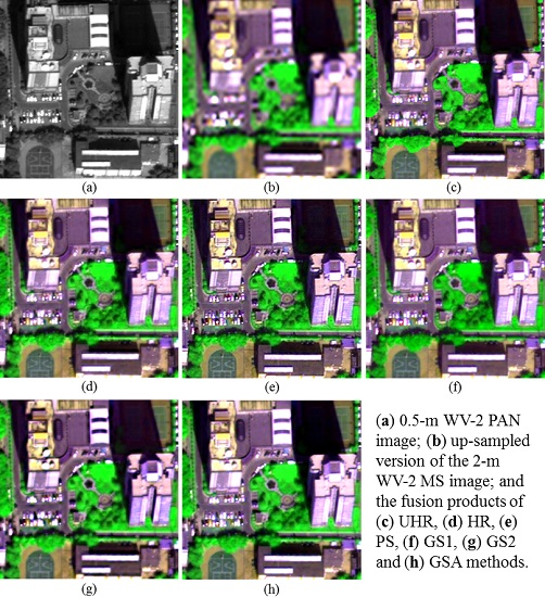
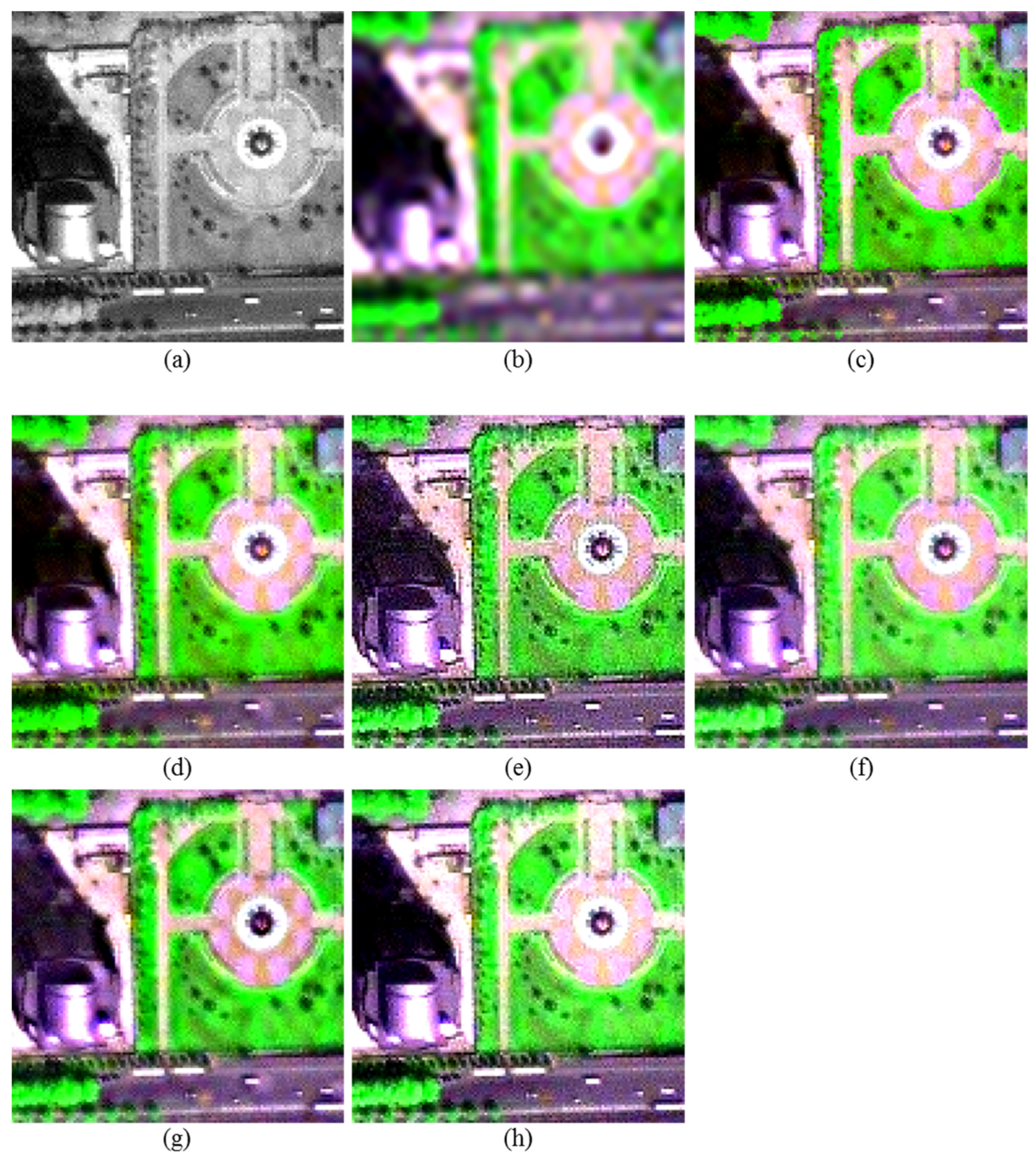
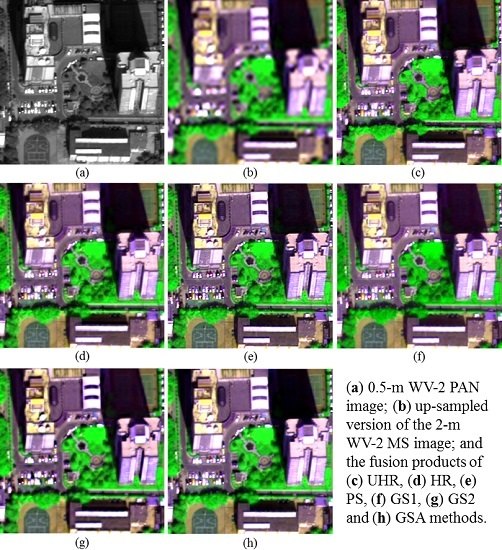
Figure 8. The 256 × 256 subsets of the MS and PAN images and the corresponding fused images produced from the original WV-2 dataset: (a) 0.5-m PAN image; (b) up-sampled version of the 2-m MS image; and the results of (c) UHR fusion, (d) HR fusion, (e) PS fusion, (f) GS1 fusion, (g) GS2 fusion and (h) GSA fusion.

Figure 8. The 256 × 256 subsets of the MS and PAN images and the corresponding fused images produced from the original WV-2 dataset: (a) 0.5-m PAN image; (b) up-sampled version of the 2-m MS image; and the results of (c) UHR fusion, (d) HR fusion, (e) PS fusion, (f) GS1 fusion, (g) GS2 fusion and (h) GSA fusion.

For the experiments at the original scale, the UHR method gives the highest QNR value followed by the HR and GS2 methods, for both the WV-2 and IKONOS datasets. The UHR performs better than the HR method in terms of QNR, D_λ, and D_S, indicating that the UHR is effective at reducing both spectral and spatial distortions. It can also be seen from the UHR-fused images shown in Figure 8 and Figure 9 that this method produces sharper VNV boundaries than the other fusion methods.

Figure 9. The 128 × 128 subsets of the MS and PAN images and the corresponding fused images produced from the original IKONOS dataset: (a) 1-m PAN image; (b) up-sampled version of the 4-m MS image; and the results of (c) UHR fusion; (d) HR fusion; (e) PS fusion; (f) GS1 fusion; (g) GS2 fusion and (h) GSA fusion.

Figure 9. The 128 × 128 subsets of the MS and PAN images and the corresponding fused images produced from the original IKONOS dataset: (a) 1-m PAN image; (b) up-sampled version of the 4-m MS image; and the results of (c) UHR fusion; (d) HR fusion; (e) PS fusion; (f) GS1 fusion; (g) GS2 fusion and (h) GSA fusion.

The GS2 method outperforms the GS1 method in terms of the QNR, because the former has a significantly lower D_S value than the latter. This may be because GS2 employs a low-pass version of the PAN image obtained by applying an MTF-matched filter to the original PAN image rather than by using a weighted average of the MS bands. The latter approach is also employed by the GSA and PS methods to produce the LSR PAN images. The LSR PAN images produced by the latter approach may introduce spectral distortions due to the difference between the spectral response ranges of the MS bands and that of the PAN band. This is especially obvious in Figure 9, where the PS-, GS1- and GSA-fused images show obvious spectral distortions.

The GS1 method has a higher QNR than the PS and GSA methods because it produces lower D_λ values than the other two methods, especially for the IKONOS dataset. Although PS and GSA perform better than GS2 and GS1 at the degraded scale in terms of ERGAS, SAM and Q2ⁿ, the former methods perform more poorly than the latter in terms of D_λ. This is because D_λ measures the difference between the inter-band relationships of the fused bands and those of the LSR MS bands, and this difference is not considered by the quality indices.

The GSA yields the lowest QNR for the WV-2 dataset, as it produces the highest D_λ value, whereas it provides the lowest QNR for the IKONOS dataset, as it produces the highest D_S. This difference between the D_λ and D_S values of the GSA-fused images of the two sensors may be caused by the different spectral response ranges of the PAN images acquired by the two sensors.

3.5. Determination of the Involved Parameters

The determination of the values of the parameters used in the fusion process, on which the quality of the fusion products generated by the proposed method mainly depends, is discussed in this section in order to facilitate the application of the proposed method. Each of the parameters L_V, L_P and S_N was set to a range of different values, and the quality of the resultant fusion products obtained using both the WV-2 and IKONOS datasets at the original and degraded scales was assessed using both the QNR and Q2ⁿ indices.

In Section 2, it was already explained that the value of L_V, which determines the accuracy of the identification of VNV boundaries in the PAN image, can be set no higher than 2R − 1. Given a value of R of 4 for all of the datasets, L_V was, therefore, tested with values of 5 (2R − 3), 7 (2R − 1) and 9 (2R + 1) in the experiment.

The value of L_P, which determines the maximum distance (in pixels) between the identified MSPs and the corresponding VNV boundaries, also depends mainly on the value of R and, based on this consideration, should be set equal to 2R − 1. However, the value of L_P is also affected by the interpolation method used to produce the up-sampled MS image. A 23-tag pyramid filter was used to generate the up-sampled MS images in this study. The spectrum of a vegetation pixel that lies across the coarse VNV boundaries derived from the LSR MS image can affect the spectral values of pixels within the neighboring 23 × 23-pixel window. Since the coefficients with significantly higher values are concentrated at the 11 pixels in the center of the filter, L_P was set to the odd numbers in the range [5,11], and the quality of the resultant fused images was assessed. The value of S_N determines the size of the window within which the search for the purest vegetation or non-vegetation pixel to be used to un-mix an MSP during the fusion process is carried out. Its value is also affected by the value of R and the interpolation method used for producing the up-sampled MS, as well as by the spatial resolution. Consequently, the value of S_N was also set to odd numbers in the range [5,11].

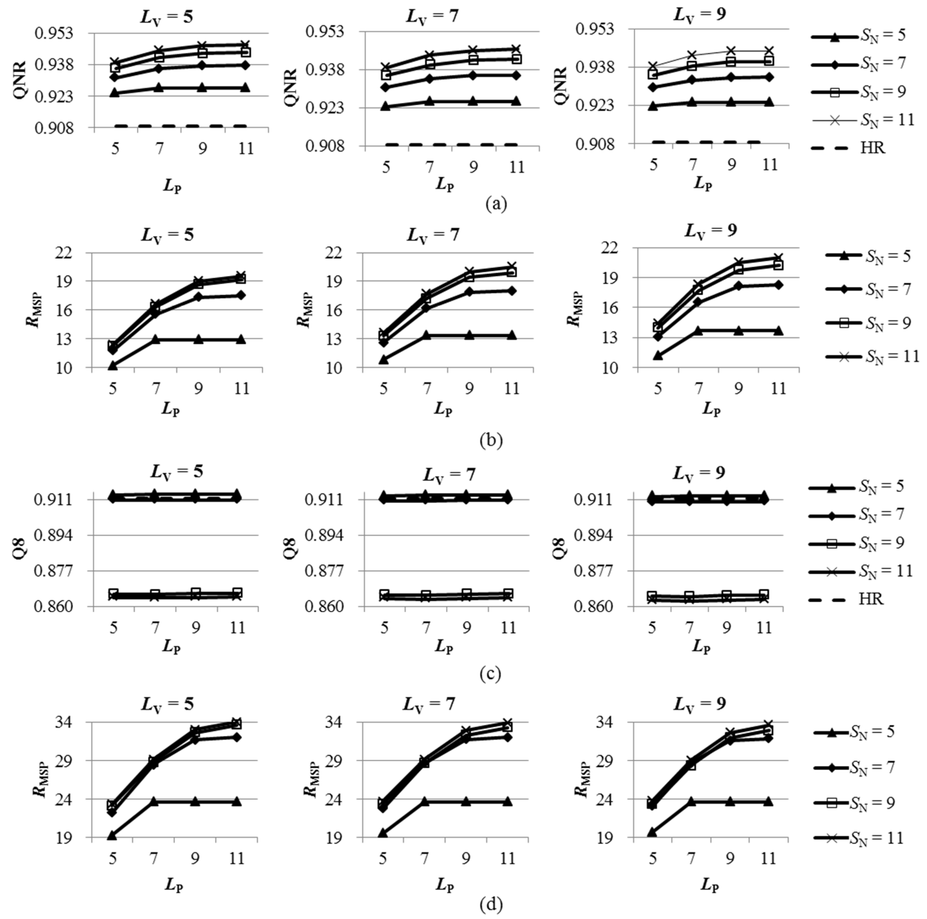
The fusion products derived from the two image types at both scales were generated by using different values for L_V, L_P and S_N, along with a δ of 3 and an S_P of 7. The values of QNR and Q2ⁿ were used to assess the quality of the fused images. R_MSP, the ratio (as a percentage) of the number of un-mixed MSPs in each fusion product to the image size (in pixels) was also recorded as a reference of the determination of these parameters. The values of QNR and Q8 along with the R_MSP values of the fusion products for the two WV-2 datasets are shown in the line graphs in Figure 10; those for the two IKONOS datasets are shown in Figure 11.

Figure 10. (a) QNR and (b) ratio of un-mixed MSPs (R_MSP) for the UHR-fused images produced from the original WV-2 dataset; (c) Q8 and (d) R_MSP for the UHR-fused images produced from the degraded WV-2 dataset.

Figure 10. (a) QNR and (b) ratio of un-mixed MSPs (R_MSP) for the UHR-fused images produced from the original WV-2 dataset; (c) Q8 and (d) R_MSP for the UHR-fused images produced from the degraded WV-2 dataset.

It can be observed from Figure 10 and Figure 11 that the quality of the fusion products, in terms of both Q2ⁿ and QNR, for both the WV-2 and IKONOS datasets at the two scales, is most sensitive to the value of S_N, followed by the values of L_V and L_P. For the two datasets at the degraded scale, only the fusion products generated using a value of 5 for S_N yield better performances than the HR-fused image in terms of Q2ⁿ. In contrast, for the two datasets at the original scale, all of the fusion products yield better performances than the HR method in terms of QNR.

R_MSP is also more sensitive to the value of S_N than it is to L_V and L_P. Generally, a higher value of S_N results in a higher R_MSP. However, a higher S_N does not always result in a better quality fusion product, because a higher R_MSP may introduce spectral distortions caused by over-un-mixing. This is especially significant for the case of the fusion products at the degraded scale, where a value of 11 for S_N results in the highest R_MSP, but the lowest Q2ⁿ value.

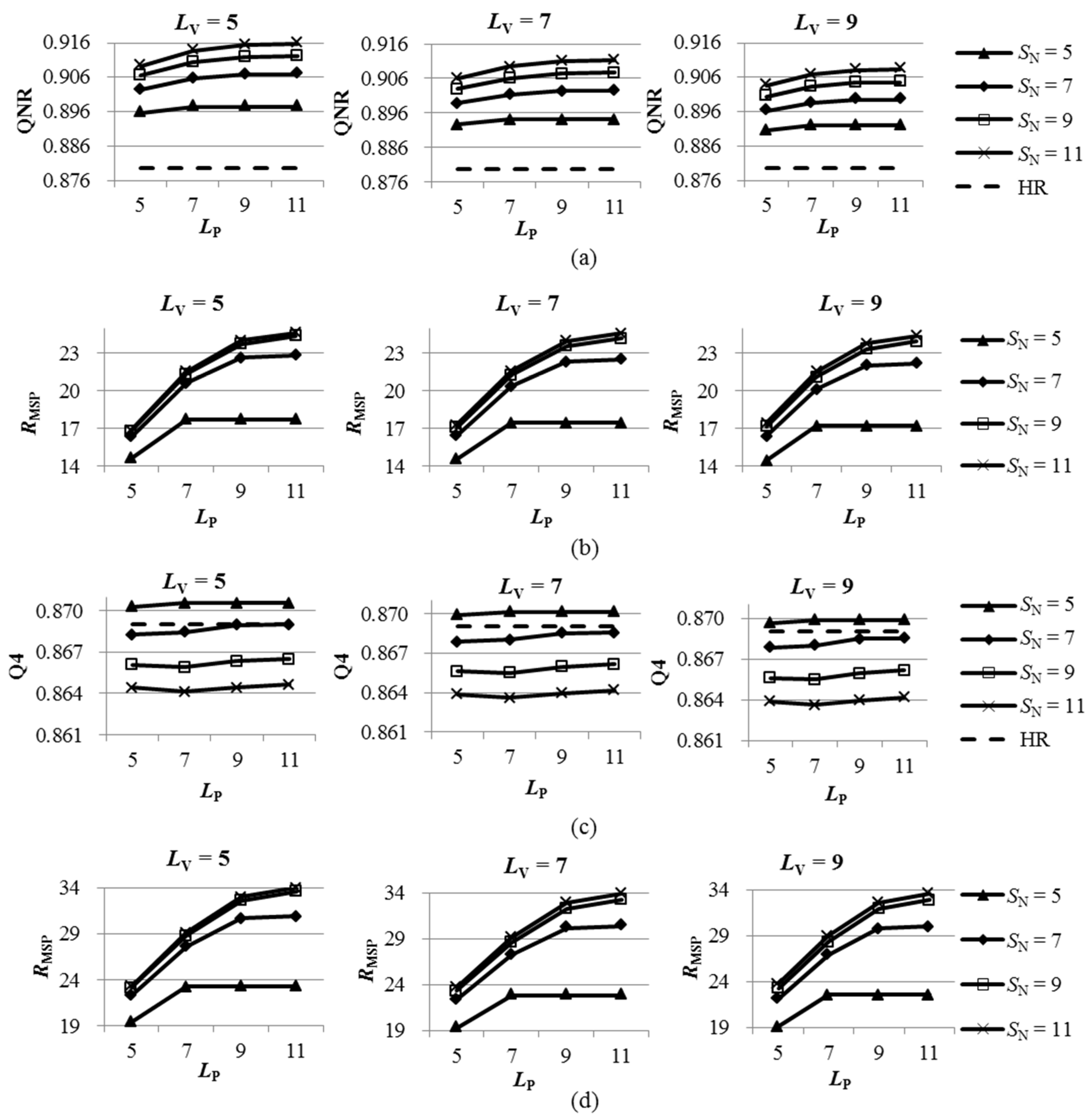
The best performances for the two degraded datasets are achieved by a value of 5 for L_V and values of 7, 9 and 11 for L_P, along with a value of 5 for S_N. The best performances for the two original datasets are achieved by the fusion products generated using a value of 5 for L_V and values of 7, 9 and 11 for L_P, along with a value of 11 for S_N. Although a value of 11 gives the poorest performance at the degraded scale, it performs the best at the original scale. This may be caused by the fact that the QNR is less sensitive to spectral distortions introduced by over-un-mixing of MSPs than the Q2ⁿ. Consequently, it is suggested that the values of L_V and S_N be set to 5 (i.e., 2R − 3), whereas the value of L_P can be set to odd values in the range (2R − 1, 11) in cases where a 23-tag filter is employed to yield the up-sampled MS image.

Figure 11. (a) QNR and (b) ratio of un-mixed MSPs (R_MSP) for the UHR-fused images produced from the original IKONOS dataset; (c) Q4 and (d) R_MSP for the UHR-fused images produced from the degraded IKONOS dataset.

Figure 11. (a) QNR and (b) ratio of un-mixed MSPs (R_MSP) for the UHR-fused images produced from the original IKONOS dataset; (c) Q4 and (d) R_MSP for the UHR-fused images produced from the degraded IKONOS dataset.

4. Discussion

Pansharpening can be generalized as the injection of spatial details derived from the PAN image into an up-sampled MS image to produce a high spatial resolution MS image. Numerous methods were proposed to optimize the spatial details derived from the PAN image or to optimize the weights by which the spatial details multiply during the injection, in order to reduce spectral distortions of the fused images. However, commonly-used image fusion methods rarely consider the spectral distortions introduced by the up-sampled MS image. Consequently, the generated fusion products suffer from spectral distortions and blurred boundaries between different objects. Hence, the application of these fused images in mapping, classification and object extraction is limited. It is desirable that the MSPs that correspond to the pure PAN pixels are fused to pure pixels with the same land cover classes (i.e., the same as those of the corresponding pure PAN pixels) to reduce the spectral distortions in the fused images. A pansharpening method including the un-mixing of MSPs is proposed in this study.

However, the un-mixing of MSPs is not an easy task, because it is difficult to identify the MSPs and to decide which land cover categories the corresponding pure PAN pixels belong to using only the LSR MS and PAN images. Moreover, incorrect un-mixing of the MSPs, caused by incorrect decisions about the land cover categories and the use of incorrect substitutions during the un-mixing, may introduce spectral distortions. Since the spectral differences between vegetation and non-vegetation objects are more significant than those between other objects, the MSPs near the VNV boundaries contribute more spectral distortions than those near the other boundaries. Hence, only the MSPs near the VNV boundaries are considered to be un-mixed to pure vegetation or pure non-vegetation in the proposed UHR fusion method.

In the tests on the IKONOS and WV-2 datasets, two quality assessments were performed on the fusion products obtained at both the original and degraded scales in order to evaluate the proposed method. The quality assessments of the datasets acquired by the two sensors demonstrated that the UHR-fused images had the lowest spectral and spatial distortions. Visual comparison demonstrated that the UHR-fused images also had clearer VNV boundaries than the fusion products generated by the PS, GS and HR methods. The UHR method performed better on the original datasets in terms of the QNR than on the degraded datasets in terms of Q2ⁿ, perhaps because of the relatively low spatial resolution of the degraded imagery, as well as the different quality indexes used at the two scales. The relatively low spatial resolutions of the degraded datasets increased the ratio of the number of MSPs to the number of pixels in the whole image. As a result, it became more difficult to search for correct substitutes for the fusion of the identified MSPs. As a consequence, some MSPs that correspond to pure non-vegetation were defined as being pure vegetation in the fused images, and vice versa. The incorrect fusion of these MSPs led to limited improvement in the quality indexes (i.e., Q2ⁿ) of the UHR-fused images for the degraded IKONOS and WV-2 datasets. However, the UHR-fused images for the two degraded datasets still had significantly sharpened VNV boundaries, as could be observed by visual inspection.

It was necessary to set the values of several parameters to generate fused images using the proposed method. These parameters include the standard deviation (δ) of an LOG edge detector, the size of a moving window within which to calculate the average NDVI values (S_P), the diameters of two disk-shaped SEs (L_V and L_P) and the size of the neighborhood window within which to search for a substitution pixel (S_N). The values of δ and S_P were set to 0.3 and 2R − 1, respectively, where R was the spatial resolution ratio of the MS and PAN images. The parameters L_V, L_P, S_N were set to different values, and the quality of the resulting fusion products at the original and degraded scales were accessed using the QNR and Q2ⁿ indices, respectively. The experimental results showed that the best performances were achieved by the fusion products generated using a value of 5 for both L_V and S_N, along with values of 7, 9 and 11 for L_P. Consequently, it is recommended that L_V and S_N are set to a value of 2R − 3, whereas the value of L_P can be set to any odd number in the range (2R − 1, 11). Haze was taken into account in the proposed fusion method. In the fusion experiment, haze values were determined for each of the bands using the minimum grey level values in the bands, based on an image-based dark-object subtraction method [42,43,44].

The quality of the fused images generated by the proposed fusion method is affected by the accuracies of the three processing steps involved, including identifying MSPs near VNV boundaries, determining land cover categories of the identified MSPs and finding the correct substitution pixels for the un-mixing of these MSPs near VNV boundaries. The second step, determining the categories (i.e., vegetation or non-vegetation) of the MSPs near VNV boundaries (i.e., the sub-pixels with category C_M in M_PI) is the most difficult, since these MSPs often have high NDVI values. In this study, the VNV boundaries, along with the NDVI image, were used to determine the categories of the identified MSPs. Although some classification errors could be found in the land cover classification map, the fused images generated from the original IKONOS and WV-2 datasets by the proposed method had lower spectral and spatial distortion than the fused images generated by any of the HR, PS, GS and GSA fusion methods. However, improving the accuracy of the classification is a topic requiring further research. In order to minimize spectral distortions caused by incorrect substitutions, the land cover category of pixel t (i.e., M_LC(t)) is checked with respect to the corresponding NDVI value (i.e., I_NDVI(t)), whereas the NDVI value of the substitution pixel n is strictly checked before the fusion is performed. In detail, the value of $M_{\mathrm{LC}}\left(t\right)$ is checked using the two conditions in Equation (9). If neither of the two conditions in Equation (9) is met, indicating that pixel t may be misclassified in $M_{\mathrm{LC}}$, the un-mixing is not performed for pixel t, in order to avoid spectral distortion caused by an incorrect substitution pixel employed. The NDVI of the substitution pixel n ($I_{\mathrm{NDVI}}\left(n\right)$) is checked using Equation (10). In detail, if pixel t is a vegetation pixel in $M_{\mathrm{LC}}$, $I_{\mathrm{NDVI}}\left(n\right)$ should be higher than $I_{\mathrm{NDVI}}\left(t\right)$, since the substitution pixel should correspond to a pure vegetation pixel in the up-sampled MS image, but t corresponds to a VNV mixed pixel in the up-sampled MS image. Similarly, if pixel t is a non-vegetation pixel in $M_{\mathrm{LC}}$, $I_{\mathrm{NDVI}}\left(n\right)$ should be lower than $I_{\mathrm{NDVI}}\left(t\right)$. Although both pixels are of the same category (i.e., vegetation or non-vegetation) in the PAN band, there is a spectral difference between the pixel t in the true high spatial resolution MS image and the fused pixel t, which is generated by the HR method with respect to the spectra of the substitution pixel. In addition, the MSPs that lie across VNV boundaries, which are mixed pixels of vegetation and non-vegetation in the reference MS image, are set to pure vegetation or non-vegetation pixels in the resultant fused images, which may introduce spectral distortions. The substitution strategy works fine, but needs further optimization. Although the HR method is employed in the proposed fusion scheme to calculate the fused versions of the sub-pixels, some other fusion methods based on the SDM injection model, such as the Brovey, SFIM and PS methods, could also be used in the proposed scheme to improve the quality of the fusion products.

5. Conclusions

Pansharpening algorithms can be summarized as the injection of the spatial details of a PAN image into an up-sampled MS image to generate a high resolution MS image. How to minimize spectral distortions while preserving the spatial details of the PAN image is a major topic in pansharpening. Most current methods focus on optimizing the spatial details derived from the PAN image and the weights of the spatial details during the injection. However, the mixed sub-pixels in the up-sampled MS image also contribute to the spectral and spatial distortions in the resulting fused image, and few fusion algorithms include the reduction of the spectral distortions caused by these mixed sub-pixels. To reduce the spectral distortions generated by currently-used fusion methods, an image fusion method that realizes the spectral un-mixing of mixed MS sub-pixels near VNV boundaries in the fusion process was proposed in this paper. In tests using high resolution WorldView-2 and IKONOS datasets over Beijing, the proposed method was compared to the PANSHARP, Gram–Schmidt (Modes 1 and 2), Adapted Gram–Schmidt and haze- and ratio-based fusion methods. The fused images generated by the proposed method produced lower spectral and spatial distortions and much sharper boundaries between vegetation and non-vegetation objects, indicating that un-mixing of the MSPs near VNV boundaries is effective at reducing spectral distortions. The land cover category (i.e., vegetation or non-vegetation) of each of the MSPs is a prerequisite for the correct un-mixing of the identified MSPs. Improving the accuracy of the land cover classification and optimizing the spectral substitution strategy are the subjects of further studies. Although the HR method is employed by the proposed fusion method to generate fused sub-pixels, some other fusion methods employing the SDM injection model, such as the Brovey, SFIM and PS methods, can also be used in the proposed scheme to improve the quality of the fusion products.