JPSS-1 VIIRS Pre-Launch Response Versus Scan Angle Testing and Performance

Abstract

The Visible Infrared Imaging Radiometer Suite (VIIRS) instruments on-board both the Suomi National Polar-orbiting Partnership (S-NPP) and the first Joint Polar Satellite System (JPSS-1) spacecraft, with launch dates of October 2011 and December 2016 respectively, are cross-track scanners with an angular swath of ±56.06°. A four-mirror Rotating Telescope Assembly (RTA) is used for scanning combined with a Half Angle Mirror (HAM) that directs light exiting from the RTA into the aft-optics. It has 14 Reflective Solar Bands (RSBs), seven Thermal Emissive Bands (TEBs) and a panchromatic Day Night Band (DNB). There are three internal calibration targets, the Solar Diffuser, the BlackBody and the Space View, that have fixed scan angles within the internal cavity of VIIRS. VIIRS has calibration requirements of 2% on RSB reflectance and as tight as 0.4% on TEB radiance that requires the sensor’s gain change across the scan or Response Versus Scan angle (RVS) to be well quantified. A flow down of the top level calibration requirements put constraints on the characterization of the RVS to 0.2%–0.3% but there are no specified limitations on the magnitude of response change across scan. The RVS change across scan angle can vary significantly between bands with the RSBs having smaller changes of ~2% and some TEBs having ~10% variation. Within a band, the RVS has both detector and HAM side dependencies that vary across scan. Errors in the RVS characterization will contribute to image banding and striping artifacts if their magnitudes are above the noise level of the detectors. The RVS was characterized pre-launch for both S-NPP and JPSS-1 VIIRS and a comparison of the RVS curves between these two sensors will be discussed.

1. Introduction

The Visible Infrared Imaging Radiometer Suite (VIIRS), aboard both the Suomi National Polar-orbiting Partnership (S-NPP) and the first Joint Polar Satellite System (JPSS-1) spacecraft with launch dates of October 2011 and late 2016 respectively, is a cross-track scanning sensor in a low Earth orbit [1]. VIIRS provides calibrated Top-Of-Atmosphere (TOA) radiance, reflectance and brightness temperature Sensor Data Records (SDRs) for weather and climate applications similar to its heritage sensors Advanced Very High Resolution Radiometer (AVHRR) [2], Operational Linescan System (OLS) [3], and Moderate Resolution Imaging Spectroradiometer (MODIS) [4]. VIIRS has 22 bands on four focal plane assemblies (FPAs). The Visible Near Infrared (VisNIR) FPA (bands I1, I2 and M1–M7) covers a spectral range of 395–900 nm. The Day Night Band (DNB) has its own FPA with multiple detector arrays for each of its three gain stages and is a panchromatic band with a spectral range of 500–900 nm [5]. There are two cold focal planes with the Short- and Mid-wave Wavelength Infrared (SMWIR) FPA (bands I3, I4 and M8–M13) covering a spectral region of 1230–4130 nm while the Long Wavelength Infrared (LWIR) FPA (bands I5 and M14–M16) covers the 8400–12,490 nm wavelength range. The band center wavelength, spatial resolution and gain type information are listed in Table 1. At NADIR, the fourteen moderate resolution bands (M-bands) and the DNB have a ground dynamic field of view (DFOV) of 750 m with 16 detectors in track while the five imaging resolution bands (I-bands) have DFOVs of 375 m with 32 detectors in track.

Table 1. The Visible Infrared Imaging Radiometer Suite (VIIRS) Spectral, Spatial and Radiometric Specifications at Typical Scenes (Ltyp or Typ).

Band Name	Gain	Center Wavelength (nm)	Focal Plane Assembly	DFOV (m)	Calibration Accuracy @Ltyp or Ttyp (%)
DNB	MG	700	DNB	750	5/10/30
M1	DG	412	VNIR	750	2
M2	DG	445	VNIR	750	2
M3	DG	488	VNIR	750	2
M4	DG	555	VNIR	750	2
M5	DG	672	VNIR	750	2
I1	SG	640	VNIR	375	2
M6	SG	746	VNIR	750	2
M7	DG	865	VNIR	750	2
I2	SG	865	VNIR	375	2
M8	SG	1240	SMIR	750	2
M9	SG	1378	SMIR	750	2
M10	SG	1610	SMIR	750	2
I3	SG	1610	SMIR	375	2
M11	SG	2250	SMIR	750	2
I4	SG	3740	SMIR	375	5
M12	SG	3760	SMIR	750	0.7
M13	HG	4050	SMIR	750	0.7
M14	SG	8550	LWIR	750	0.6
M15	SG	10,763	LWIR	750	0.4
I5	SG	11,450	LWIR	375	2.5
M16	SG	12,013	LWIR	750	0.4

Table 1. The Visible Infrared Imaging Radiometer Suite (VIIRS) Spectral, Spatial and Radiometric Specifications at Typical Scenes (Ltyp or Typ).

Band Name	Gain	Center Wavelength (nm)	Focal Plane Assembly	DFOV (m)	Calibration Accuracy @Ltyp or Ttyp (%)
DNB	MG	700	DNB	750	5/10/30
M1	DG	412	VNIR	750	2
M2	DG	445	VNIR	750	2
M3	DG	488	VNIR	750	2
M4	DG	555	VNIR	750	2
M5	DG	672	VNIR	750	2
I1	SG	640	VNIR	375	2
M6	SG	746	VNIR	750	2
M7	DG	865	VNIR	750	2
I2	SG	865	VNIR	375	2
M8	SG	1240	SMIR	750	2
M9	SG	1378	SMIR	750	2
M10	SG	1610	SMIR	750	2
I3	SG	1610	SMIR	375	2
M11	SG	2250	SMIR	750	2
I4	SG	3740	SMIR	375	5
M12	SG	3760	SMIR	750	0.7
M13	HG	4050	SMIR	750	0.7
M14	SG	8550	LWIR	750	0.6
M15	SG	10,763	LWIR	750	0.4
I5	SG	11,450	LWIR	375	2.5
M16	SG	12,013	LWIR	750	0.4

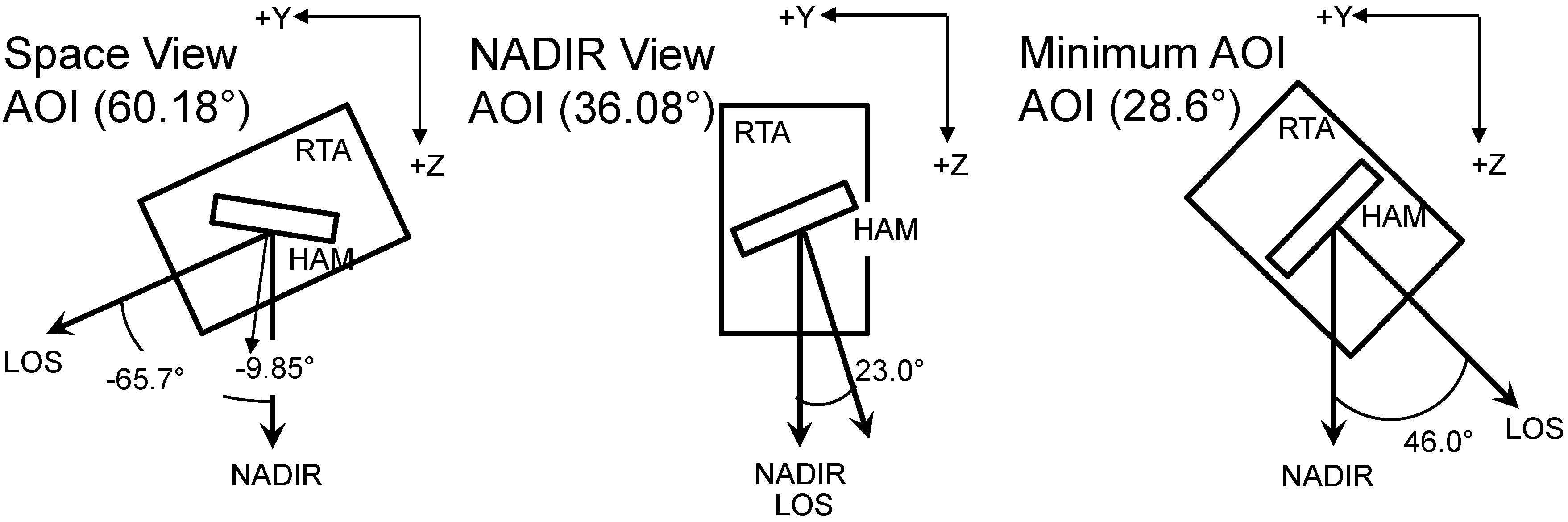
VIIRS is in a sun-synchronous orbit with an altitude of ~828 km, an equatorial crossing of 13:30 and swath width of about 3000 km [6]. To achieve this swath, VIIRS covers an Earth View (EV) cross-track scan angle range of ±56.06° and uses for the scanner an afocal three mirror anastigmat telescope and fold mirror foreoptic called the Rotating Telescope Assembly (RTA). The RTA rotates 360° to allow the light from the EV as well as from the internal calibration sources to be collected. The light out of the RTA is redirected to the instrument’s stationary aft-optics (including the 4 FPAs) using a Half Angle Mirror (HAM) that rotates at half the speed of the RTA. To achieve this, the HAM has a silver mirror coating on both sides that alternates each scan. These are referred to as HAM sides A and B (or sides 0 and 1 with respect to the vendor’s nomenclature) and have slightly different reflectance properties since the coating was deposited on the HAM sides at different times. The Angle of Incidence (AOI) on the RTA mirror surfaces and aft-optics are fixed over scan angle but are dependent on detector and band location on the FPAs. The HAM however does have a scan angle dependent AOI variation with 28.60° to 56.47° change over the full EV scan angle. The three calibration targets within the VIIRS cavity, the Space View (SV), On-Board Calibrator BlackBody (OBCBB) and Solar Diffuser (SD) have AOIs around 60.18°, 38.53° and 60.47° respectively. The AOI of the OBCBB is within the AOI range of the EV and matches the EV AOI at a scan angle of −8°, while the SV and SD share almost the same AOI but are located at far different scan angles (−65.7° and 159° respectively), and are outside the range of the EV scan.

Figure 1 illustrates the relationship between the RTA Line of Sight (LOS) and the HAM normal vector. The left most image shows the RTA/HAM geometry at the SV scan angle. The RTA is rotated to -65.7° from the NADIR view and the HAM normal is 9.85° from NADIR. The middle image shows the NADIR scan angle with the RTA LOS at the +Z direction and the HAM normal vector at 23.0°. The last image shows the RTA/HAM combination where the HAM AOI is at a minimum (28.6°) at a scan angle of 46.0° with both the RTA LOS and the HAM normal having the same geometry. However, there is an Out-Of-Plane (OOP) angle of 28.6° on the HAM in the X coordinate direction to fold the light from the RTA towards the aft-optics not shown in the figure. This additional OOP angle along with the angle difference between the RTA LOS and the HAM normal vector are used to compute the AOI of the HAM. The equations to do this conversions will be discussed in the next section. The EV sector uses timing delays to co-register the band imagery so that the SDR products represent the same area on the ground for all bands. This makes the mapping between scan angle and AOI the same for all bands within the EV sector. The calibration sectors however are not co-registered and therefore each band and detector have a unique AOI when viewing these sources that needs to be accounted for when applying their RVS corrections. The calibration sectors record 48 M-band samples or 96 I-band samples during each scan allowing noise suppression through averaging and Signal to Noise Ratio (SNR) determination to be performed on a per scan basis. The EV when in operational mode contains 3200 M-band samples for single gain bands and 6400 for I-bands (see Table 1). These EV samples include aggregation that minimizes the effective pixel growth on the ground due to the Earth’s curvature. There are six aggregation zones and their scan angle ranges are listed in Table 2. The dual gain M-bands are packaged unaggregated with 6304 samples due to the need to calibrate each pixel separately depending on gain values (high or low) within an aggregated pixel [7].

Table 2. Sample Aggregation Zones for Non-Day Night Bands (DNBs).

Zone	Start Scan Angle (°)	End Scan Angle (°)	Number of Samples Aggregated
1	−56	−43	1
2	−43	−32	2
3	−32	0	3
4	0	32	3
5	32	43	2
6	43	56	1

Table 2. Sample Aggregation Zones for Non-Day Night Bands (DNBs).

Zone	Start Scan Angle (°)	End Scan Angle (°)	Number of Samples Aggregated
1	−56	−43	1
2	−43	−32	2
3	−32	0	3
4	0	32	3
5	32	43	2
6	43	56	1

The four-mirror RTA, HAM and aft-optics telescope system all use silver mirror coatings to reflect the photons from the EV or calibration sources to the four FPAs. The silver coatings are preferred to other mirror coating options due to its high reflectance over a large spectral range (0.395–13 μm) and very high reflectance (>98%) in the blue spectral region. Similar to its heritage sensor MODIS, VIIRS uses Quantum FSS-99 for its silver mirrors. 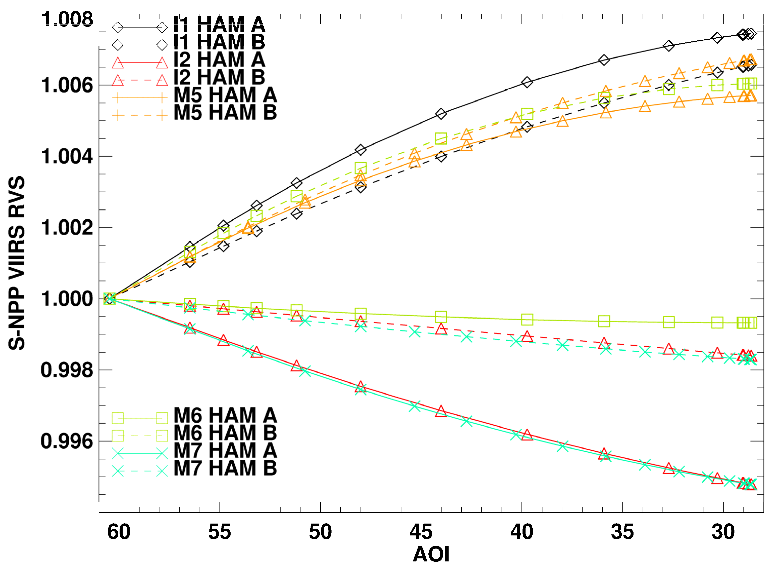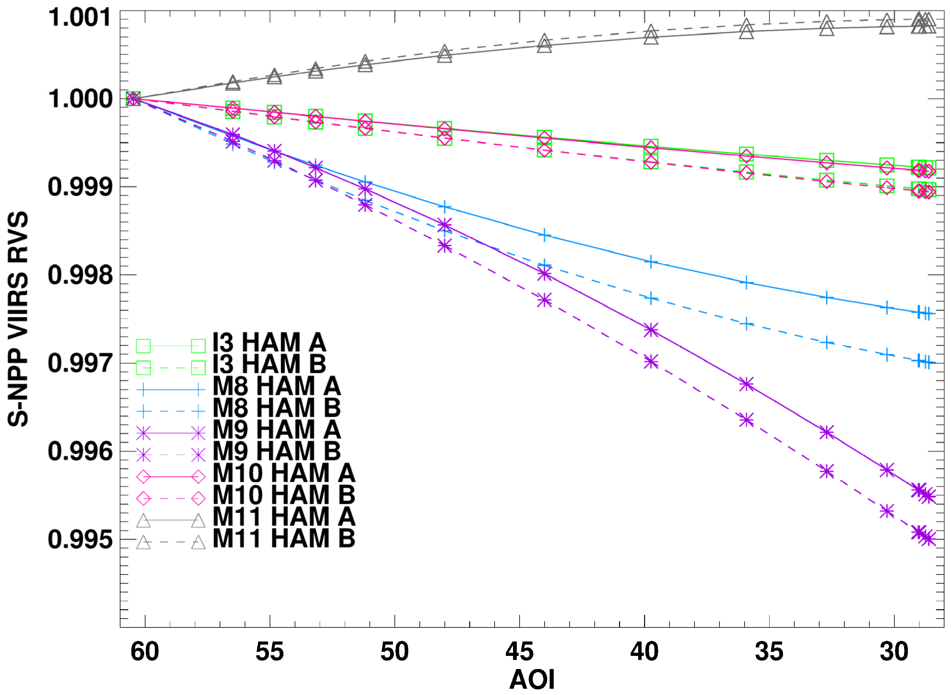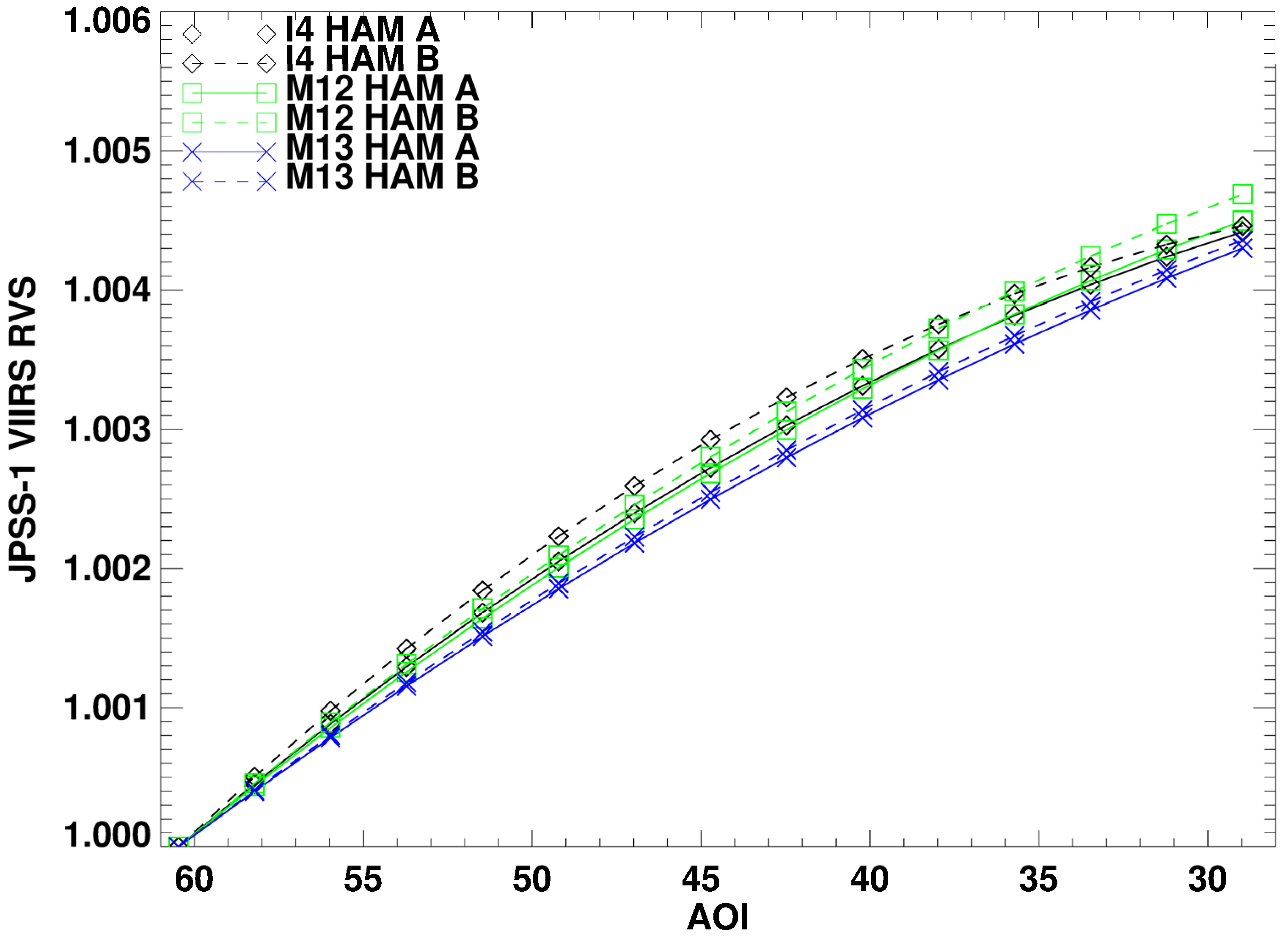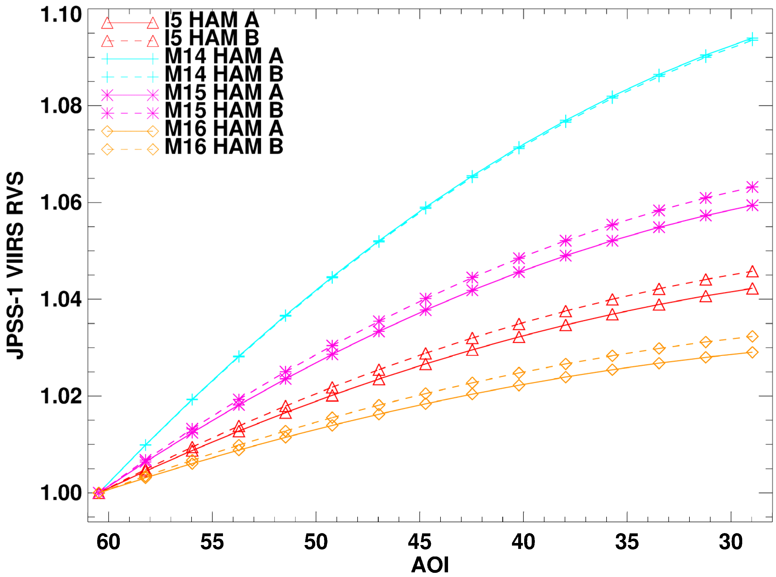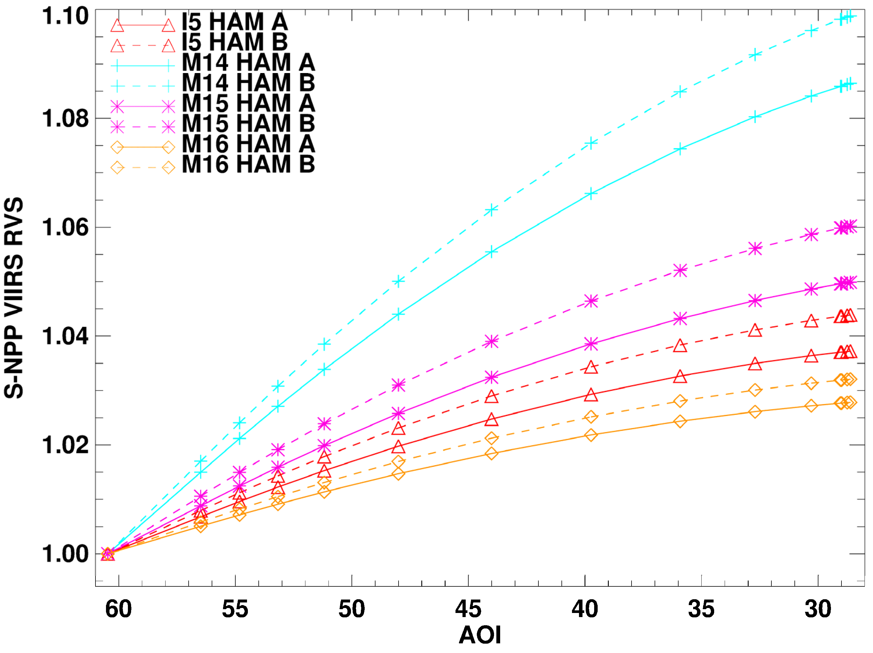The process used to deposit the FSS-99 coating onto the mirror substrate is proprietary but consists of a silver mirror with a dielectric overcoat to protect the silver coating from exposure to the environment [8]. The silver mirror and overcoat cause a wavelength dependent reflectance in the mirror surface as a result of spectral variation in the index of refraction. The thickness of the silver and overcoat and the path length variation through these surfaces as a function of AOI on the mirror creates the reflectance variation observed in the RVS measurements. The RTA and aft-optics have fixed AOIs for each band and detector but the HAM AOI does vary throughout the scan. With large AOIs on the HAM of 60.18°, consistency in the coating characteristics (purity of the deposit and coating thickness) are important to maintain reflectance and RVS repeatability between HAM sides and sensor builds. This paper will compare the S-NPP RVS to JPSS-1 RVS performance and will show how mirror coating deposition on the HAM varies both with HAM side (temporally close in deposition time) and sensor builds (very large temporal separation in deposition time).

Figure 1. Example of the Rotating Telescope Assembly (RTA) and Half Angle Mirror (HAM) Orientations at three different scan angles. The left most diagram corresponds to the Space View (SV) scan angle, the middle is the NADIR scan angle and the right most is the scan angle where the HAM Angle of Incidence (AOI) is at a minimum.

Figure 1. Example of the Rotating Telescope Assembly (RTA) and Half Angle Mirror (HAM) Orientations at three different scan angles. The left most diagram corresponds to the Space View (SV) scan angle, the middle is the NADIR scan angle and the right most is the scan angle where the HAM Angle of Incidence (AOI) is at a minimum.

The radiometric requirements listed in Table 1 for both the RSB and TEB allocate 0.3% and 0.2% (except for band M14 at 0.6%) uncertainty respectively for the RVS characterization. The RVS change over the scan is not restricted in the requirements but must be characterized to within the allotted uncertainty (polarization effects are not included in the RVS and are separately characterized [9] for Environmental Data Record (EDR) processing [10]). The RVS is tested at system level and not at the HAM component level to allow the characterization with the on-orbit view geometry of the detector footprints on the HAM and RTA to be performed. This removes any errors from modeling the view geometry configurations as well as spatial non-uniformity of the HAM coating surface that is not included in the component level measurements.

The RVS requirements are for the full mission of the instrument and thus need to account for not only prelaunch characterization uncertainty but also on-orbit degradation effects. One major on-orbit influence to the silver mirror coating performance is UV exposure [11,12,13]. Degradation of the reflectance, especially in the blue region, is common for both MODIS and VIIRS on-orbit. The MODIS optical design has the scan mirror as the first surface in optical train which makes it the first surface exposed to UV light and thus degradation is significant over the mission [11]. This is an issue because the AOI on this scan mirror is changing as a function of scan angle and thus the RVS for MODIS has changed shape throughout the mission. It not only changed but each HAM side has changed at different rates [14]. The VIIRS design has the four-mirror RTA before the HAM which absorbs most of the UV light with minimal UV reaching the HAM surface. Since the RTA does not contribute to RVS, only reflectance or gain change, the RVS performance for S-NPP has remained stable. No adjustments to RVS in the SDR ground processing has been performed due to on-orbit degradation. The calibration methodology for both the RSB and TEB will be discussed as well as the RVS characterization results. Comparisons between S-NPP and JPSS-1 will be shown to understand shape differences and their impact to their sensor’s calibration.

2. RVS Testing Approach

2.1. Response Versus Scan Angle Test Source Assembly

Pre-launch JPSS-1 VIIRS RVS testing data was collected at Raytheon Space and Airborne Systems in El Segundo, California in late 2013 for the RSB and early 2014 for the TEB. The RVS characterization utilized 3 sources: the Laboratory Ambient BlackBody (LABB) as a target for TEBs, a 100 cm Spherical Integrating Source (SIS-100) for the RSBs and the OBCBB as an ambient blackbody for background subtraction purposes. VIIRS was placed on a Rotating Table to allow the sensor to be rotated with respect to the LABB or SIS100 to facilitate different scan angle measurements.

Table 3 lists the RSB scan angle measurements in the sequence they were acquired. The scan angle positions are purposely not measured in monotonic order and there are several repeats at the −8° scan angle location. The repeats provide stability measurements as well as source drift correction capabilities while the non-sequential scan angles allow for source drift and any other time-dependent Ground Support Equipment (GSE) or VIIRS sensor effects in ambient conditions—to be decoupled from RVS shape characteristics. The SIS-100 source is set to a single radiance level to provide optimum illumination to the blue wavelength and Shortwave Infrared (SWIR) bands at nominal integration time settings. The integration time of the instrument was then adjusted to optimize the remaining RSBs response to the SIS-100 while maintaining testing efficiency. This resulted in three different integration time settings at each scan angle position. Use of fixed sources while varying sensor integration time greatly reduces source drifts during measurements by keeping the lamps within the SIS-100 in a steady state thermal configuration.

Table 3. Response Versus Scan (RVS) Data Collection Configuration with Scan Angles and Diagnostic Window Information for both the Reflective Solar Bands (RSBs) and Thermal Emissive Bands (TEBs).

Collection	RSB Scan Angle (°)	RSB Diagnostic Window	RSB M-Band Sample Offset	TEB Scan Angle (°)	TEB Diagnostic Window	TEB M-Band Sample Offset
1	−65.7	Nominal	0	−8	Third	2128
2	−8	Third	2128	−65.7	First	0
3	−38	First	0	22	Fifth	4254
4	6	Third	2128	-45	First	0
5	−45	First	1064	6	Fourth	3192
6	−8	Third	2128	−8	Third	2128
7	−55.5	First	0	−55.5	First	0
8	22	Fourth	3192	−20	Third	2128
9	−30	First	1064	−38	Second	1064
10	−8	Third	2128	−8	Third	2128
11	−51	First	0	−51	First	0
12	38	Fifth	4254	35	Fifth	4254
13	−20	Second	1064	−30	Second	1064
14	55.5	Fifth	4254	−8	Third	2128
15	−8	Third	2128	−60.6	First	0

Table 3. Response Versus Scan (RVS) Data Collection Configuration with Scan Angles and Diagnostic Window Information for both the Reflective Solar Bands (RSBs) and Thermal Emissive Bands (TEBs).

Collection	RSB Scan Angle (°)	RSB Diagnostic Window	RSB M-Band Sample Offset	TEB Scan Angle (°)	TEB Diagnostic Window	TEB M-Band Sample Offset
1	−65.7	Nominal	0	−8	Third	2128
2	−8	Third	2128	−65.7	First	0
3	−38	First	0	22	Fifth	4254
4	6	Third	2128	-45	First	0
5	−45	First	1064	6	Fourth	3192
6	−8	Third	2128	−8	Third	2128
7	−55.5	First	0	−55.5	First	0
8	22	Fourth	3192	−20	Third	2128
9	−30	First	1064	−38	Second	1064
10	−8	Third	2128	−8	Third	2128
11	−51	First	0	−51	First	0
12	38	Fifth	4254	35	Fifth	4254
13	−20	Second	1064	−30	Second	1064
14	55.5	Fifth	4254	−8	Third	2128
15	−8	Third	2128	−60.6	First	0

Table 3 lists the TEB scan angle measurements in the sequence they were acquired. As with the RSBs, the TEB measurements are purposely non-sequential in scan angle. The scan angle order is slightly different than the RSB measurements but the distribution of scan angles throughout the measurement sequence is very similar. The TEB scan angle measurements add a 35° point near the minimum AOI as well at −60.6° (where the AOI change with scan angle is very steep) to better characterize the RVS for these bands. The TEB RVS dependencies can vary by as much at 10% over scan (M14) and it is important to characterize their shape where the slope of the curve is strongest. The RSB RVS dependences tend to have about 2% variation over scan making them less sensitive to AOI changes at the beginning of scan. The LABB was set to 345 K while the OBCBB was at ambient temperature (~293 K). The TEBs needed only 2 integration time settings to optimize the signal for testing. This allowed the LABB to be at a fixed temperature and provide a more steady state thermal environment during the test. This was important to minimize variation in the background emission within the VIIRS cavity during the test. Both the LABB and SIS-100 are extended sources that allow many VIIRS samples to have their full field of view filled by source illumination. Both the RSB and TEB RVS measurements used an average of 100 M-band or 200 I-band samples across the source and then averaged over 50 scans for each HAM side.

During RVS testing, the VIIRS instrument was configured to be in a special data collection mode called diagnostic mode. This mode turns off on-board sample aggregation in scan, thereby removing any sample averaging complications from the test data analyses. The down side of diagnostic mode is that full scans of data cannot be transmitted with aggregation turned off. As a result only 2048 samples out of the 6304 M-samples within a full scan are reported. To accommodate this lack of full scan range, diagnostic windows of 2048 M-band samples at different scan-angle regions within a sub section of the entire EV scan are used. Columns 3 and 6 in Table 3 list the diagnostic window at each scan angle that was collected. Sample numbers along with the diagnostic window offsets are used to compute the actual AOI of each measurement during the RVS test. For the TEB RVS measurements, a sector rotation was performed to move the SV port into the EV scan data collection range. This did not allow the 55.5° scan angle measurement in the RSB RVS test to be measured but allowed the LABB to be placed at the SV port and still be viewed in the EV sector data window. This allowed 100 M-band samples to be averaged for the SV angle during the TEB test unlike the 48 M-band samples used in the RSB and 15 for the DNB. With the large AOI of the SV and significant sensitivity to RVS for the TEBs, the improvement in the SV RVS measurement accuracy was very important.

2.2. VIIRS RSB RVS Analysis Methodology

The SDRs for the RSBs provide a calibrated TOA radiance and reflectance product. The RVS plays an integral part of calibration algorithm for radiance shown in Equation (1) [15].

$$L=\frac{F·(c_0+c_{1}d{n}_{EV}+c_{2}d{n}_{EV}^2)}{RVS\left({\theta }_{EV}\right)}$$

(1)

The c₀, c₁ and c₂ are the calibration coefficients determined pre-launch during Thermal Vacuum (TVAC) testing. The dn_EV are the EV Digital Numbers (DNs) minus the SV DNs, the RVS as a function of scan angle (or sample number) is in the denominator and the F factor is the gain drift correction determined using the SD as described in Equation (2).

$$F=\frac{RVS\left({\theta }_{SD}\right)·E_{SUN}·{\tau }_{SD}·\cos \left({\phi }_{SD}\right)·BR{F}_{SD}·H}{(c_0+c_{1}d{n}_{SD}+c_{2}d{n}_{SD}^2)}$$

(2)

The numerator is the estimated Solar radiance reflected off the SD pin hole screen (τ_SD) to attenuate the Solar irradiance (E_SUN) that reflects off the lambertian SD (BRF_SD). The denominator is the TVAC calibration coefficients scaled by the dn_SD (SD DNs) minus the SV DNs. Similar to the RVS in Equation (1), the calibration coefficients are divided by the RVS (θ_SD) which moves to the numerator of Equation (2). The RVS (θ_SD) is determined from the SD AOI and is band and detector dependent due to a lack of co-registration in the calibration sectors.

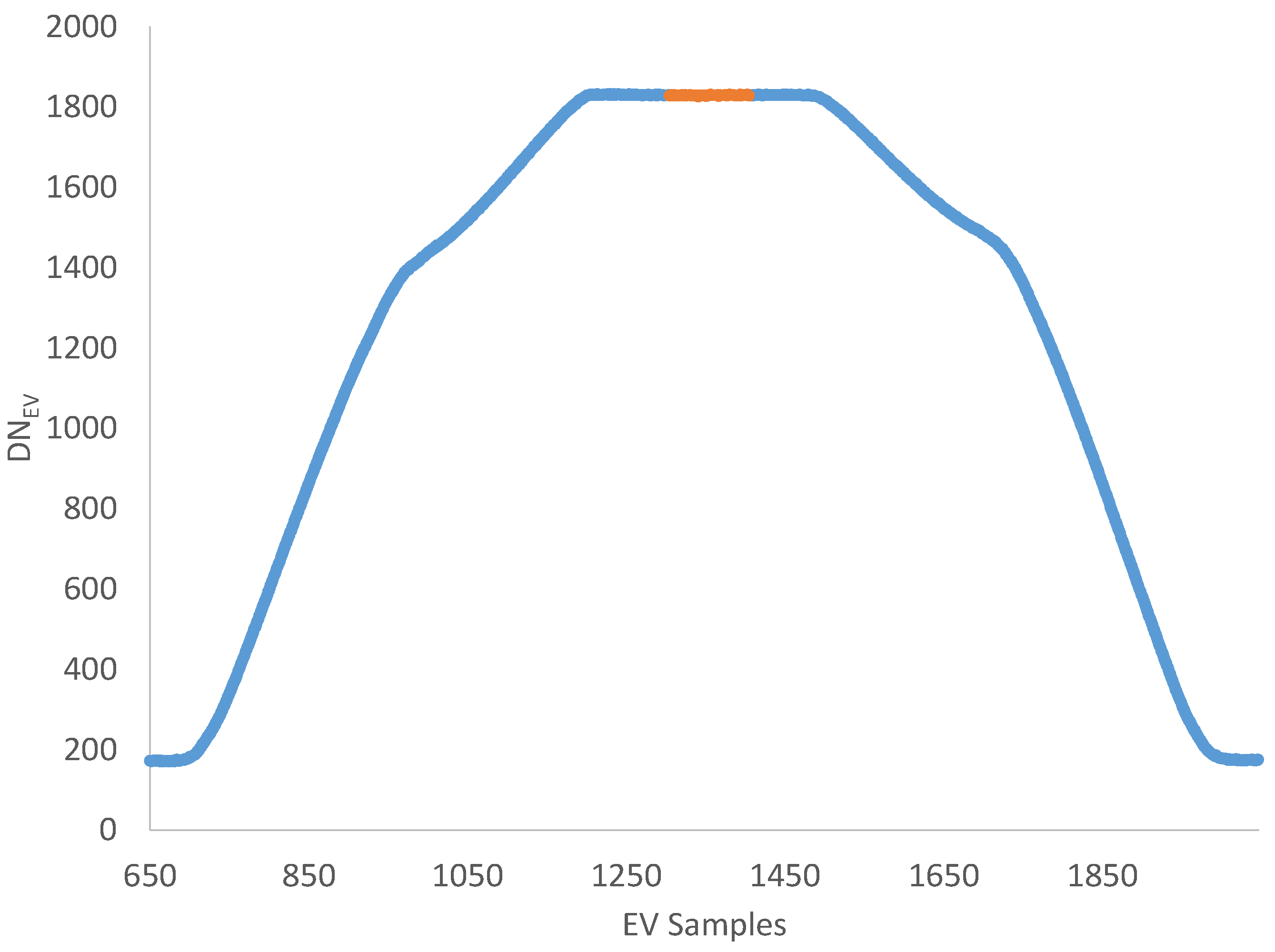
The RVS data analysis for the RSBs consists of processing the VIIRS response from the SIS-100 source, mapping the source location in scan angle space to determine the AOI, drift correcting the VIIRS response to account for source instability and fitting the data to a 2nd-order polynomial to allow interpolation of the data to any AOI value. An example of the VIIRS response to the SIS-100 is shown in Figure 2 for band M1. The center of the source profile is identified for each scan angle measurement configuration and 100 M-samples that straddle the center are extracted (only 40 samples for the DNB). These samples have an offset subtraction applied using the mean of the OBCBB samples since the SV port is exposed to allow the SIS-100 to be placed in that location. This is performed for each scan and then the dn_EV is averaged over samples and 50 scans for each detector and HAM side. The −65.7° scan angle corresponding to the SV uses the SIS-100 in the SV port and provides only 48 M-samples to be averaged. The mapping of the scan angle to AOI uses the center sample value, diagnostic window offset and Equations (3)–(5).

$${\theta }_{scan}=\left(x+\mathsf{\beta }-S_{off}\right)·{\delta }_{scan}-{\theta }_{start}$$

(3)

$${\theta }_{HAM}=\frac{{\theta }_{scan}-{\phi }_{ref}}{2}$$

(4)

$$AOI={\cos }^{-1}\left(\cos \left({\theta }_{HAM}\right)·\cos \left({\phi }_{oop}\right)\right)$$

(5)

Figure 2. Band M1 DN Response to the SIS-100 Source during the RVS Test (the orange points correspond to the RVS data used during processing).

Figure 2. Band M1 DN Response to the SIS-100 Source during the RVS Test (the orange points correspond to the RVS data used during processing).

The angles φ_oop and φ_ref are fixed angles of 28.6° and 46.0° respectively. The θ_scan is the scan angle of VIIRS and is computed for each image sample using Equation (3). The sample number (x) of the image, offset by diagnostic window shift (β), the boresight offset (S_off) that integrates the sensor pointing information and scaled by the angular scan rate (δ_scan at 0.017785 deg/sample) is combined with the angular offset of the start of scan (θ_start at −60.058°) is then subtracted to get the scan angle (3). The scan angle (θ_scan) combined with the reference scan angle offset (φ_ref), is used to determine the θ_HAM angle (4). The θ_HAM corresponds to the vector difference between the RTA LOS and the HAM normal vector. The cosine of that θ_HAM with the OOP angle (φ_oop) corresponding to the angle to fold the light towards the aft optics gives the AOI in (5).

The SIS-100 source drift correction uses the −8° scan angle measurements that are repeated throughout the test to track the source output at a common sensor configuration. These −8° scan angle measurements are assumed to track a linear source drift between repeats. Any non-linear drifts will not be correctly removed from the measurements and will show up as residual error during the RVS fits. Each set of −8° repeat point dn pairs are linear fit and normalized by the first −8° repeat, and used to correct dn values from all scan angle measurement captured between those −8° repeat pairs. The dns of each measurement between repeats is scaled by the drift correction based on the time that measurement was acquired. After the source correction is applied, a 2nd-order polynomial fit of dns normalized to the SV scan angle versus AOI is performed to model the RVS characteristics. Since the scan angle measurements are not in a monotonic order, residual source drift correction errors and temporal errors will show up as fit residual errors. This provides confidence that the shape of the RVS curve is capturing true VIIRS gain change versus scan angle and not external error sources during the test. The larger the fit residuals, the more uncertainty in the characterization due to these external error sources. One example of this is the band M9 RVS due its spectral response being in a water vapor absorption region. The water vapor varies during the RVS test and will influence the characterization due to these temporal changes. The residuals will be larger but its influence on the RVS shape is reduced since the scan angles are not measured in a sequential fashion. The residuals of the fits are driven by dn noise, GSE uncertainties and other temporal error sources and are used to assess the quality of the RVS characterization.

2.3. VIIRS TEB RVS Analysis Methodology

Unlike the RSBs where the RVS scales the radiance computed using pre-launch calibration coefficients only, the TEBs have a more complicated relationship between RVS and calibrated radiance. Equation 6 shows how the VIIRS response for the TEBs is converted to a calibrated radiance.

$$L_{ap}\left(RV{S}_{EV}\right)=\frac{\left(RV{S}_{SV}-{\mathrm{RVS}}_{EV}\right)\cdot \left[\frac{\left(1-{\rho }_{rta}\right)\cdot L\left(T_{rta}\right)-L\left(T_{ham}\right)}{{\rho }_{rta}}\right]+F\cdot {\displaystyle \sum _{i=0}^2{c}_i\left(T_{\det },T_{elec}\right)\cdot {(D{N}_{EV}-D{N}_{SV})}^i}}{{\mathrm{RVS}}_{EV}}$$

(6)

Similar to the RSBs, the TEBs have c₀, c₁ and c₂ calibration coefficients to convert EV DNs subtracted by the SV DNs (dn_EV) into radiance. This is scaled by a gain drift correction (F factor) described in Equation (7). The additional piece to the TEB calibration is the residual background emission terms from the RTA and HAM due to RVS differences between the EV and SV scan angles or OBCBB and SV scan angles. The L(T_rta) and L(T_ham) are radiance terms for the RTA and HAM respectively that are estimated using internal thermistors within the VIIRS cavity. The ρ_rta is the reflectance of the RTA which combines the reflectance of the four-mirror RTA telescope.

$$\begin{array}{l}F={\mathrm{RVS}}_{OBCBB}\frac{\left\{\left(1-\frac{RV{S}_{SV}}{{\mathrm{RVS}}_{OBCBB}}\right)\cdot \left[\frac{\left(1-{\rho }_{rta}\right)\cdot L\left(T_{rta}\right)-L\left(T_{ham}\right)}{{\rho }_{rta}}\right]\right\}}{{\displaystyle \sum _{j=0}^2{c}_j\cdot {(D{N}_{OBCBB}-D{N}_{SV})}^j}}+\\ \frac{{\epsilon }_{obc}\cdot L\left(T_{OBCBB}\right)+L_{OBCBB\_refl}\left(T_{sh},T_{cav},T_{tele}\right)}{{\displaystyle \sum _{j=0}^2{c}_j\cdot {(D{N}_{OBCBB}-D{N}_{SV})}^j}}\end{array}$$

(7)

The L_{OBCBB_refl} is the internal cavity emission reflected off the OBCBB, the ε_obc is the emissivity of the OBCBB and the L(T_OBCBB) is the OBCBB radiance estimated using the 6 potted thermistors. The magnitude in the RVS differences between source and SV views determines how much the RTA and HAM background emission terms contribute to the total radiance. The TEB RVS curves, which can vary by as much as 10% across the scan, must be accurately characterized or brightness temperature biases in the SDR product that are scan angle and scene dependent will occur. Table 4 shows the worst case impact within the EV scan on the SDR brightness temperatures for the TEBs when using an RVS error of 0.2%. The cold scene SDR brightness temperatures are more sensitive to RVS error due to the background emission term being reweighted by the RVSsv-RVSev difference in equation 6. Band M14 is the only LWIR band to show large (3 K) change at the low scene temperatures. All of the LWIR bands have > 0.1 K SDR brightness temperature change at warm scenes and would impact the downstream EDR products. These RVS errors would also cause detector-to-detector striping or scan-to-scan banding based on scene temperature and would be difficult to remove with operational code corrections. Therefore, characterizing the RVS to 0.2% uncertainty for the TEB is vital.

Table 4. Maximum Sensor Data Records (SDR Brightness Temperature Error (K) Due to 0.2% RVS Shape Error at Multiple Scene Temperatures (K) for all TEBs.

--	SDR Brightness Temperature Error (K)
Band	190 (K)	210 (K)	230 (K)	247 (K)	262 (K)	278 (K)	292 (K)	307 (K)	321 (K)	332 (K)	340 (K)	345 (K)
I4	3.843	0.946	0.257	0.075	0.015	0.016	0.030	0.041	0.049	0.054	0.057	0.060
I5	0.407	0.207	0.105	0.051	0.014	0.019	0.043	0.068	0.089	0.105	0.116	0.123
M12	4.011	1.086	0.268	0.078	0.015	0.016	0.030	0.041	0.048	0.053	0.057	0.059
M13	5.948	0.950	0.235	0.073	0.015	0.016	0.032	0.043	0.052	0.057	0.061	0.064
M14	3.012	0.361	0.137	0.058	0.015	0.019	0.042	0.064	0.082	0.095	0.104	0.110
M15	0.509	0.231	0.112	0.052	0.014	0.019	0.043	0.067	0.088	0.103	0.114	0.121
M16	0.364	0.195	0.102	0.050	0.014	0.019	0.043	0.068	0.089	0.105	0.117	0.124

Table 4. Maximum Sensor Data Records (SDR Brightness Temperature Error (K) Due to 0.2% RVS Shape Error at Multiple Scene Temperatures (K) for all TEBs.

--	SDR Brightness Temperature Error (K)
Band	190 (K)	210 (K)	230 (K)	247 (K)	262 (K)	278 (K)	292 (K)	307 (K)	321 (K)	332 (K)	340 (K)	345 (K)
I4	3.843	0.946	0.257	0.075	0.015	0.016	0.030	0.041	0.049	0.054	0.057	0.060
I5	0.407	0.207	0.105	0.051	0.014	0.019	0.043	0.068	0.089	0.105	0.116	0.123
M12	4.011	1.086	0.268	0.078	0.015	0.016	0.030	0.041	0.048	0.053	0.057	0.059
M13	5.948	0.950	0.235	0.073	0.015	0.016	0.032	0.043	0.052	0.057	0.061	0.064
M14	3.012	0.361	0.137	0.058	0.015	0.019	0.042	0.064	0.082	0.095	0.104	0.110
M15	0.509	0.231	0.112	0.052	0.014	0.019	0.043	0.067	0.088	0.103	0.114	0.121
M16	0.364	0.195	0.102	0.050	0.014	0.019	0.043	0.068	0.089	0.105	0.117	0.124

The RVS data analysis for the TEBs is slightly different from the RSB methodology. It consists of processing the VIIRS response from the LABB source, mapping the source location in scan angle space to determine the AOI, drift correcting using the LABB and OBCBB temperature information and fitting the data to a 2nd-order polynomial to allow interpolation of the data to any AOI value. The fitting algorithm requires an iteration approach that varies the RVS_SV to find the minimum residuals in the polynomial fit. This is needed because there are two RVS values in Equation (6). The purpose of the iteration is to optimize the RVS_SV-RVS_EV to best correct the background emission term in the radiance retrieval and thus reduce residual errors caused by cavity temperature drifts during the test. The VIIRS response to the LABB is shown in Figure 3 for band M15 and uses 100 M-band samples that straddle the center in a similar fashion as the RSBs. These samples have an offset subtraction applied using the mean of the OBCBB samples since the SV port is used to allow the LABB to be placed in that location. This is performed for each scan and then the dn_EV is averaged over samples and 50 scans for each detector and HAM side. The EV sector is rotated for the TEB test to allow the −65.7° scan angle to be viewed in this sector so that 100 sample averaging can be performed for this angle as well. This changes the mapping of the scan angle to AOI compared to the nominal configuration used for the RSB (−60.058°) to −70.056° as the θ_start offset in Equation (3). The remaining scan angle to AOI conversion is similar to the RSB portion using Equations (3)–(5).

Figure 3. Band M15 DN Response to the LABB Source during the RVS Test (the orange points correspond to the RVS data used during processing).

Figure 3. Band M15 DN Response to the LABB Source during the RVS Test (the orange points correspond to the RVS data used during processing).

The temperature of the LABB is set to 345 K, and the OBCBB at an ambient temperature of ~293 K is used to estimate the source radiances. This is then used as the Lap value in Equation (6) to solve for RVS_EV. The F factor is assumed to be 1 and the RVS_SV is iterated until the 2nd-order polynomial fit with the minimum fit residuals is determined. The non-sequential measurement of scan angle allows the temporal internal cavity temperature drifts to be decoupled from the RVS shape allowing the RVS_SV iteration to mostly impact the residuals and optimize the RVS shape for these bands.

3. S-NPP and J1 VIIRS RVS Results

3.1. Reflective Solar Band Results

The RSB RVS curves were computed for each detector and HAM side and all 3 I-bands and 11 M-bands. These results include the application of the SIS-100 radiance drift correction but does not include water vapor correction for band M9. This correction and its improvements to the M9 RVS has been discussed in [16]. Figure 4 shows the measurement points and 2nd-order polynomial fits for band M1 HAM side A for all detectors. The x-axis is HAM AOI with the left side of the axis at 61° representing the SV angle and beginning of scan while the 28° point on the right side representing the end of scan (the NADIR AOI is 36.08°). The measurement points were not acquired sequentially across the x-axis and show some noise indicating the drift correction error and other sources of temporal errors still remain in the data. The 2nd-order polynomial fit (solid lines) is a least squares fit of these points. The residuals indicate the characterization error in the measurement and are slightly different for each detector due to their noise performance during the test. The points are fairly monotonic and indicate the 2nd-order RVS model is appropriate for characterization purposes. Another example of RVS data is shown in Figure 5 for band I2 HAM side A for all detectors. The peak-to-peak change in RVS for this band is ~0.18% over the entire scan region. Here the temporal errors from the GSE and detector noise are more evident since there is little change in the gain across AOI. A small change in RVS makes detector noise more prominent in the measurements causing the fits look worse for I2 than for M1. However, the 2nd-order fit models the RVS very well (0.05% residuals) even though the variation across scan is very small. Figure 6 shows the RVS for band M9 HAM side A all detectors. The fit residuals in figure 6 for band M9 are much larger due to water vapor variability during the test impacting the radiance reaching the detectors. This water vapor effect is not corrected in this analysis but will be updated to account for water vapor for on-orbit purposes. While the residuals are large, the variation in RVS across the scan is ~0.3% peak-to-peak. This indicates that RVS shape errors for band M9 will not significantly impact the SDR performance on-orbit.

Figure 4. Band M1 HAM side A RVS and Fits for all Detectors.

Figure 4. Band M1 HAM side A RVS and Fits for all Detectors.

Figure 5. Band I2 HAM side A RVS and Fits for all Detectors.

Figure 5. Band I2 HAM side A RVS and Fits for all Detectors.

Figure 6. Band M9 HAM side A RVS and Fits for all Detectors.

Figure 6. Band M9 HAM side A RVS and Fits for all Detectors.

Figure 7 shows the RVS across scan for the DNB HAM side A all detectors. The variation in RVS over the scan is very small on the order of ~0.3% change peak-to-peak. This change across scan will have minimal impact on the SDR calibration. The edge detectors 1 and 16 do have unique RVS shapes but are most likely due to DN noise in the SV AOI since there were only 14 samples of data averaged for that point. Overall the DNB RVS matches well with the VisNIR RSBs with wavelengths.

Figure 7. DNB HAM side A RVS and Fits for all Detectors.

Figure 7. DNB HAM side A RVS and Fits for all Detectors.

Table 5. Maximum RVS Variation across Scan and Characterization Uncertainty for all RSBs.

Band	HAM A Maximum Peak-to-Peak Change in RVS Over Scan (%)	HAM A RMS Residuals (%)	HAM B Maximum Peak-to-Peak Change in RVS Over Scan (%)	HAM B RMS Residuals (%)
DNB	0.28	0.06	0.38	0.06
M1	1.49	0.08	0.93	0.07
M2	1.00	0.05	1.00	0.05
M3	0.74	0.04	0.70	0.05
M4	0.52	0.04	0.54	0.04
M5	0.59	0.04	0.35	0.03
I1	0.57	0.05	0.40	0.04
M6	0.67	0.04	0.50	0.03
M7	0.18	0.04	0.53	0.05
I2	0.18	0.05	0.57	0.06
M8	0.42	0.02	0.53	0.02
M9	0.27	0.28	0.34	0.28
M10	0.15	0.04	0.24	0.03
I3	0.11	0.04	0.20	0.04
M11	0.11	0.03	0.09	0.03

Table 5. Maximum RVS Variation across Scan and Characterization Uncertainty for all RSBs.

Band	HAM A Maximum Peak-to-Peak Change in RVS Over Scan (%)	HAM A RMS Residuals (%)	HAM B Maximum Peak-to-Peak Change in RVS Over Scan (%)	HAM B RMS Residuals (%)
DNB	0.28	0.06	0.38	0.06
M1	1.49	0.08	0.93	0.07
M2	1.00	0.05	1.00	0.05
M3	0.74	0.04	0.70	0.05
M4	0.52	0.04	0.54	0.04
M5	0.59	0.04	0.35	0.03
I1	0.57	0.05	0.40	0.04
M6	0.67	0.04	0.50	0.03
M7	0.18	0.04	0.53	0.05
I2	0.18	0.05	0.57	0.06
M8	0.42	0.02	0.53	0.02
M9	0.27	0.28	0.34	0.28
M10	0.15	0.04	0.24	0.03
I3	0.11	0.04	0.20	0.04
M11	0.11	0.03	0.09	0.03

Figure 8, Figure 9 and Figure 10 shows the detector-averaged RVS curves for each RSB and HAM side to show the general behavior for each band. The SDR products uses band, detector and HAM side dependent RVS corrections. The solid lines are HAM A and the dashed lines are HAM B. The largest change in RVS for the RSBs is band M1 (blue line) with ~1.015 change from the SV AOI on the left side of the plot to the end of EV scan on the right side. The dashed line for HAM B shows considerable change with respect to HAM side A (solid blue line) across the scan. This difference in HAM side RVS is due to temporal separation between when the two mirror sides were coated. HAM side A was coated by the vendor in 2009 while HAM B was coated in early 2010. This meant that the chamber used to coat these mirrors was not consistent and therefore the deposition of the silver mirror onto the HAM was slightly different between the two sides. Figure 11, Figure 12 and Figure 13 shows the band-averaged RVS curves for S-NPP. Unlike JPSS-1 VIIRS, S-NPP VIIRS HAM sides were coated very close temporally and have very similar silver mirror reflectance between sides. The overall change in RVS is different between S-NPP HAM sides but the shape across scan angle is very consistent. The magnitude of the RVS between S-NPP and JPSS-1 VIIRS is very similar with the VNIR bands showing an increase in RVS across scan while the SWIR bands mostly decrease with scan. Table 5 lists the maximum peak-to-peak variation in RVS over the scan for each band and HAM side. The RMS of the fit residuals are also listed to show the characterization uncertainty in the fits for each band.

Figure 8. Band-averaged RVS for JPSS-1 VIIRS from the SV AOI to the end of scan AOI for bands M1–M4 and DNB.

Figure 8. Band-averaged RVS for JPSS-1 VIIRS from the SV AOI to the end of scan AOI for bands M1–M4 and DNB.

Figure 9. Band-averaged RVS for JPSS-1 VIIRS from the SV AOI to the end of scan AOI for bands I1, I2 and M5–M7.

Figure 9. Band-averaged RVS for JPSS-1 VIIRS from the SV AOI to the end of scan AOI for bands I1, I2 and M5–M7.

Figure 10. Band-averaged RVS for JPSS-1 VIIRS from the SV AOI to the end of scan AOI for bands I3 and M8-M11.

Figure 10. Band-averaged RVS for JPSS-1 VIIRS from the SV AOI to the end of scan AOI for bands I3 and M8-M11.

Figure 11. Band-averaged RVS for the Suomi National Polar-orbiting Partnership (S-NPP) VIIRS RSBs from the SV AOI to the end of scan AOI for bands M1–M4.

Figure 11. Band-averaged RVS for the Suomi National Polar-orbiting Partnership (S-NPP) VIIRS RSBs from the SV AOI to the end of scan AOI for bands M1–M4.

Figure 12. Band-averaged RVS for S-NPP VIIRS RSBs from the SV AOI to the end of scan AOI for bands I1, I2 and M5–M7.

Figure 12. Band-averaged RVS for S-NPP VIIRS RSBs from the SV AOI to the end of scan AOI for bands I1, I2 and M5–M7.

Figure 13. Band-averaged RVS for S-NPP VIIRS RSBs from the SV AOI to the end of scan AOI for bands I3 and M8–M11.

Figure 13. Band-averaged RVS for S-NPP VIIRS RSBs from the SV AOI to the end of scan AOI for bands I3 and M8–M11.

3.2. Thermal Emissive Band Results

The TEB RVS curves are essential to the SDR calibration. Each TEB (2 I-bands and 5 M-bands) detector and HAM side has an individually characterized RVS to reduce detector striping and scan-to-scan banding effects in the SDR. Figure 14 shows the RVS for band M14 HAM side A for all detectors. The variation across scan in Figure 14 is a little less than 10% with a detector dependence of ~0.25% at the end of scan. The points do show some noise as a result of LABB and OBCBB temperature drifting during the test that was not fully accounted for, some emission versus scan angle influence and noise in the DNs. Figure 15 shows an RVS curve for band M12 HAM side A all detectors. Similar to the other Mid-Wave Infrared (MWIR) bands, the RVS variation over the scan is relatively small compared to the LWIR bands. The peak-to-peak change is less than 0.6% for M12 which limits the impact of background emission effects in the MWIR. The RVS is much larger in the TEBs than in the RSBs and therefore most likely have larger polarization sensitivity in these mirrors than the RSBs (only the VNIR bands are characterized for polarization sensitivity). However, unlike the VNIR bands which have significant polarization in the scene radiance from the Earth, the TEBs observe unpolarized emission from the Earth and do not have polarization sensitivity requirements. The Emission Versus Scan angle (EVS) was measured prelaunch for S-NPP and computed on-orbit using a deep space maneuver to look at cold space. Significant polarization effects from emitted light off the HAM as a function of HAM AOI would cause the EVS and RVS to have different shapes. However, the on-orbit deep space maneuver EVS matched the RVS shape very well and indicated polarization effects are not a significant contributor to the RVS performance in the SDR algorithm [17].

Figure 14. Band M14 HAM side A RVS Response and Fits for all Detectors.

Figure 14. Band M14 HAM side A RVS Response and Fits for all Detectors.

Figure 15. Band M12 HAM side A RVS Response and Fits for all Detectors.

Figure 15. Band M12 HAM side A RVS Response and Fits for all Detectors.

Figure 16 and Figure 17 show the detector averaged JPSS-1 VIIRS TEB RVS curves for both HAM side A (solid lines) and B (dotted lines) across the scan of VIIRS. Unlike the RSBs which showed significant shape differences between HAM sides (especially for blue wavelength bands), the TEBs have consistent shapes. There is some separation in the curves between the HAM sides within a band that is not consistent with S-NPP VIIRS performance but the overall magnitude of the RVS curves for each band are similar to S-NPP. Figure 18 and Figure 19 show the detector-averaged S-NPP VIIRS RVS for all the TEBs and HAM sides. The magnitudes for both S-NPP and JPSS-1 VIIRS are very similar but HAM side difference were larger on the S-NPP compared to JPSS-1. Band M14 shows much better HAM side consistency on JPSS-1 compared to S-NPP. Table 6 lists the worst case peak-to-peak variation over scan for both HAM sides for each TEB as well as the worst case RMS fit residuals.

Table 6. Maximum RVS Variation across Scan and Characterization Uncertainty for all TEBs.

Band	HAM A Maximum Peak-to-Peak Change in RVS Over Scan (%)	HAM A RMS Residuals (%)	HAM B Maximum Peak-to-Peak Change in RVS Over Scan (%)	HAM B RMS Residuals (%)
I4	0.56	0.05	0.60	0.05
M12	0.59	0.07	0.60	0.05
M13	0.56	0.06	0.56	0.05
M14	9.64	0.08	9.60	0.08
M15	6.13	0.07	6.53	0.07
I5	4.55	0.12	4.93	0.11
M16A	3.03	0.05	3.35	0.06
M16B	2.93	0.05	3.28	0.06

Table 6. Maximum RVS Variation across Scan and Characterization Uncertainty for all TEBs.

Band	HAM A Maximum Peak-to-Peak Change in RVS Over Scan (%)	HAM A RMS Residuals (%)	HAM B Maximum Peak-to-Peak Change in RVS Over Scan (%)	HAM B RMS Residuals (%)
I4	0.56	0.05	0.60	0.05
M12	0.59	0.07	0.60	0.05
M13	0.56	0.06	0.56	0.05
M14	9.64	0.08	9.60	0.08
M15	6.13	0.07	6.53	0.07
I5	4.55	0.12	4.93	0.11
M16A	3.03	0.05	3.35	0.06
M16B	2.93	0.05	3.28	0.06

Figure 16. Band-averaged RVS for JPSS-1 VIIRS all TEBs from the SV AOI through to the end of scan AOI for the Mid-wave Wavelength Infrared (MWIR) bands.

Figure 16. Band-averaged RVS for JPSS-1 VIIRS all TEBs from the SV AOI through to the end of scan AOI for the Mid-wave Wavelength Infrared (MWIR) bands.

Figure 17. Band-averaged RVS for JPSS-1 VIIRS all TEBs from the SV AOI through to the end of scan AOI for the Long Wavelength Infrared (LWIR) bands.

Figure 17. Band-averaged RVS for JPSS-1 VIIRS all TEBs from the SV AOI through to the end of scan AOI for the Long Wavelength Infrared (LWIR) bands.

Figure 18. Band-averaged RVS for S-NPP VIIRS all TEBs from the SV AOI through to the end of scan AOI for the MWIR bands.

Figure 18. Band-averaged RVS for S-NPP VIIRS all TEBs from the SV AOI through to the end of scan AOI for the MWIR bands.

Figure 19. Band-averaged RVS for S-NPP VIIRS all TEBs from the SV AOI through to the end of scan AOI for the LWIR bands.

Figure 19. Band-averaged RVS for S-NPP VIIRS all TEBs from the SV AOI through to the end of scan AOI for the LWIR bands.

4. Conclusions

The Response Versus Scan angle for JPSS-1 VIIRS was measured using stable wide-field sources to provide accurate characterization. The results showed that the JPSS-1 VIIRS RVS shapes are consistent with its predecessor on the S-NPP spacecraft with the exception of band M1 being larger for JPSS-1 (Figure 8). Some HAM side differences are present on the JPSS-1 VIIRS that were not present on S-NPP, especially for blue wavelength bands that can be traced back to HAM side coating differences. These differences were caused by a long time period between when the two sides of the JPSS-1 VIIRS HAM coating were deposited. The RSBs show less than 2% variation in RVS across the scan and the MWIR TEBs also show very small (~1%) change across scan as well (similar between JPSS-1 and S-NPP). The LWIR TEBs do show significant (~10%) RVS change across scan making their curves very important to the SDR calibration for these bands. These large RVS variations in the LWIR for JPSS-1 were also present in S-NPP VIIRS. The quality of the S-NPP RVS characterization allows for very good SDR performance on-orbit. It is expected that the JPSS-1 RVS will perform at a similar level. The characterization accuracy is very good (~0.12%) and well below the requirement of 0.3% (RSB) or 0.2% (TEB). The only band with large uncertainties (0.28%) is band M9, but is impacted by water vapor drifting during the test.