
Estimation of Forest Structural Diversity Using the Spectral and Textural Information Derived from SPOT-5 Satellite Images


Abstract
:
1. Introduction
2. Data and Methods
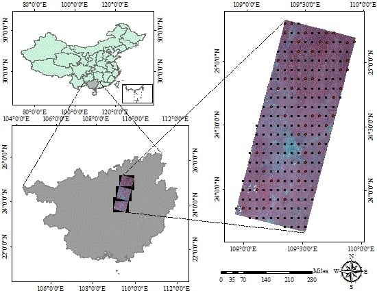
2.1. Data Source
2.1.1. National Forest Inventory Data
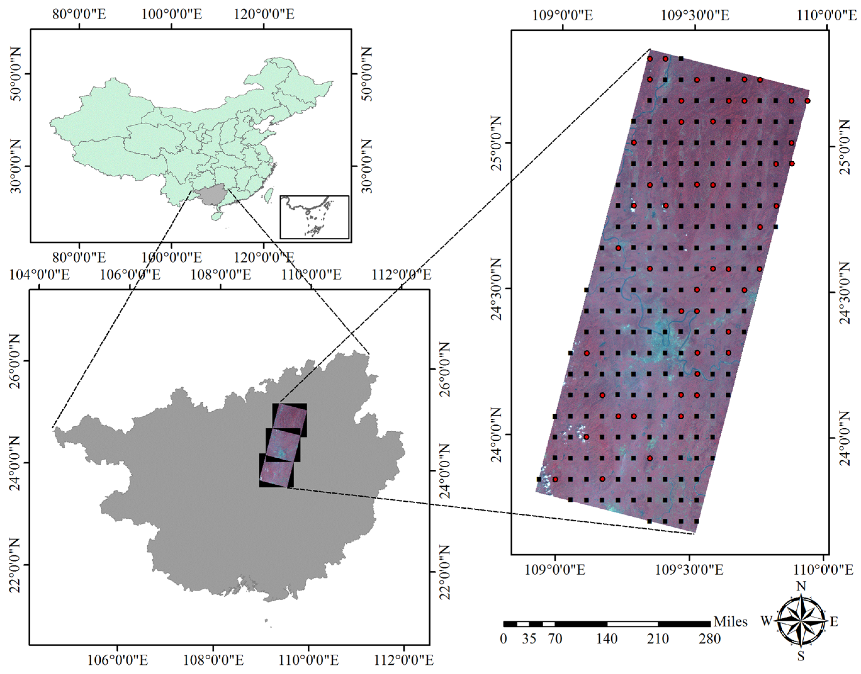
2.1.2. Remote Sensing Data
2.2. Forest Stand Variables (Dependent Variables)
2.2.1. Conventional Forest Variables
2.2.2. Forest Structural Diversity
Species Diversity
Diameter or Tree Size Diversity
Tree Position Diversity
2.3. Imagery-Derived Measures (Independent Variables)
2.3.1. Spectral Measures
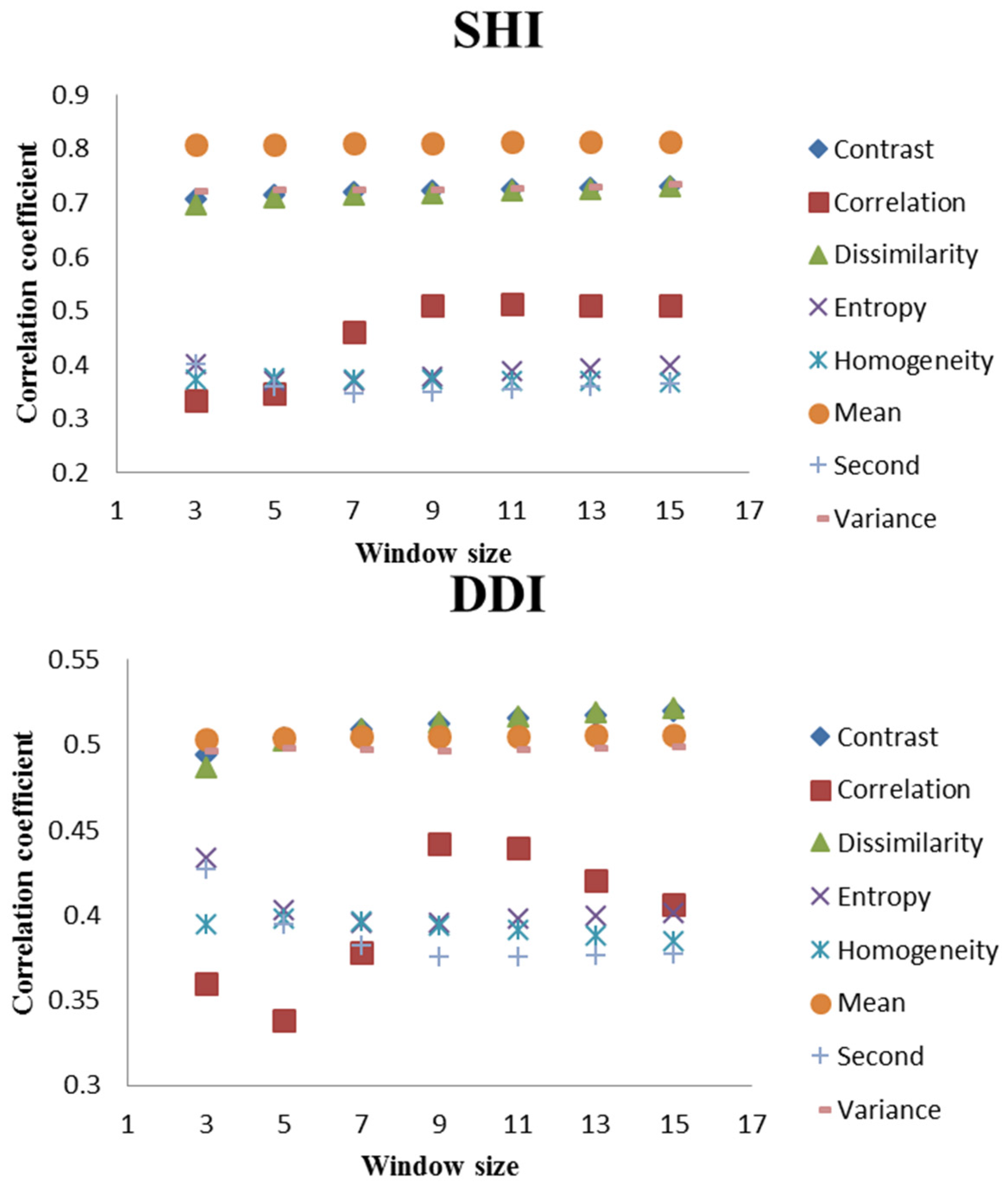
2.3.2. Textural Measures
2.4. Model Construction and Validation
3. Results
3.1. Structural Parameters

| Parameters | Mean | S.D | Min. | Max. |
|---|---|---|---|---|
| Quadratic mean diameter (QMD) (cm) | 13.10 | 3.10 | 6.58 | 21.75 |
| Basal area (BA) (m2/ha) | 18.36 | 10.04 | 4.41 | 40.44 |
| Number of trees (NT) (n/ha) | 1579 | 923 | 254 | 4313 |
| Stand volume (SV) (m3/ha) | 101.23 | 57.80 | 21.02 | 263.13 |
| Shannon–Wiener index (SHI) | 0.920 | 0.510 | 0 | 1.801 |
| Pielou index (PI) | 0.263 | 0.162 | 0 | 0.497 |
| Simpson’s index (SII) | 0.495 | 0.245 | 0 | 0.803 |
| Gini coefficient (GC) | 0.230 | 0.072 | 0.062 | 0.362 |
| Standard deviation of DBHs (SDDBH) | 4.913 | 2.227 | 0.951 | 11.197 |
| Uniform angle index () | 0.498 | 0.09 | 0.273 | 0.706 |
| Species intermingling index () | 0.398 | 0.279 | 0 | 0.778 |
| DBH dominance index () | 0.482 | 0.023 | 0.470 | 0.531 |
| Diameter differentiation index (DDI) | 0.259 | 0.094 | 0.096 | 0.429 |
3.2. Correlation Analyses
| Variables | Mean_nir | Mean_red | Mean_green | Mean_swir | Mean_pan | Brightness | Max_diff | NDVI | SR | VI | GEMI | GR | MSI | SAVI | SVR |
|---|---|---|---|---|---|---|---|---|---|---|---|---|---|---|---|
| NT | −3.712 * | −3.870 * | −0.312 | −2.998 | −0.401 ** | −0.472 * | 0.397 * | 0.301 | 0.242 | 0.356 * | −0.098 | 0.214 | 0.036 | −0.323 * | 0.059 |
| QMD | −0.413 * | −0.432 * | −0.461 * | −3.242 * | −0.422 * | −0.488 * | 0.444 * | 0.298 | 0.274 | 0.410 * | −0.214 | 0.256 * | 0.056 | −0.419 * | 0.023 |
| BA | −0.522 ** | −0.554 ** | −0.543 ** | −0.436 ** | −0.533 ** | −0.598 ** | 0.561 ** | 0.329 * | 0.314 | 0.507 ** | −0.318 * | 0.315 | 0.016 | −0.511 ** | 0.099 |
| SV | −0.512 ** | −0.580 ** | −0.536 ** | −0.450 * | −0.526 ** | −0.601 ** | 0.555 ** | 0.346 * | 0.312 | 0.512 ** | −0.307 | 0.299 | 0.012 | −0.493 * | 0.111 |
| GC | −0.401 * | −0.524 ** | −0.479 * | −0.384 * | −0.467 * | −0.454 * | 0.101 | 0.379 * | 0.383 * | 0.454 * | −0.270 | 0.221 | 0.018 | −0.424 * | 0.276 |
| DDI | −0.458 * | −0.522 ** | −0.486 ** | −0.352 * | −0.520 ** | −0.515 ** | 0.044 | 0.257 | 0.260 | 0.594 ** | −0.141 | 0.078 | 0.008 | −0.457 * | 0.115 |
| SDDBH | −0.491 * | −0.546 ** | −0.520 ** | −0.478 * | −0.546 ** | −0.557 ** | 0.341 * | 0.274 | 0.291 | 0.602 ** | −0.146 | 0.074 | −0.166 | −0.490 * | 0.023 |
| SHI | −0.646 ** | −0.829 ** | −0.824 ** | −0.492 * | −0.808 ** | −0.786 ** | 0.078 | 0.532 ** | 0.538 ** | 0.824 ** | −0.260 | 0.305 | 0.054 | −0.645 ** | 0.353 * |
| SII | −0.589 ** | −0.775 ** | −0.768 ** | −0.467 * | −0.761 ** | −0.733 ** | 0.072 | 0.502 ** | 0.504 ** | 0.766 ** | −0.303 | 0.286 | 0.004 | −0.588 ** | 0.284 |
| PI | −0.632 ** | −0.798 ** | −0.782 ** | −0.494 * | −0.771 ** | −0.763 ** | 0.110 | 0.484 * | 0.488 * | 0.817 ** | −0.300 | 0.248 | 0.008 | −0.631 ** | 0.276 |
| −0.629 ** | −0.781 ** | −0.759 ** | −0.541 ** | −0.757 ** | −0.777 ** | 0.123 | 0.434 * | 0.436 * | 0.831 ** | −0.114 | 0.197 | −0.104 | −0.628 ** | 0.141 | |
| −0.003 | −0.115 | −0.098 | −0.114 | −0.109 | −0.095 | 0.100 | 0.147 | 0.155 | 0.145 | −0.045 | 0.128 | −0.189 | −0.002 | −0.030 | |
| −0.100 | −0.129 | −0.123 | 0.0142 | −0.131 | −0.094 | −0.160 | 0.109 | 0.109 | 0.166 | −0.068 | 0.060 | 0.1402 | −0.010 | 0.152 |

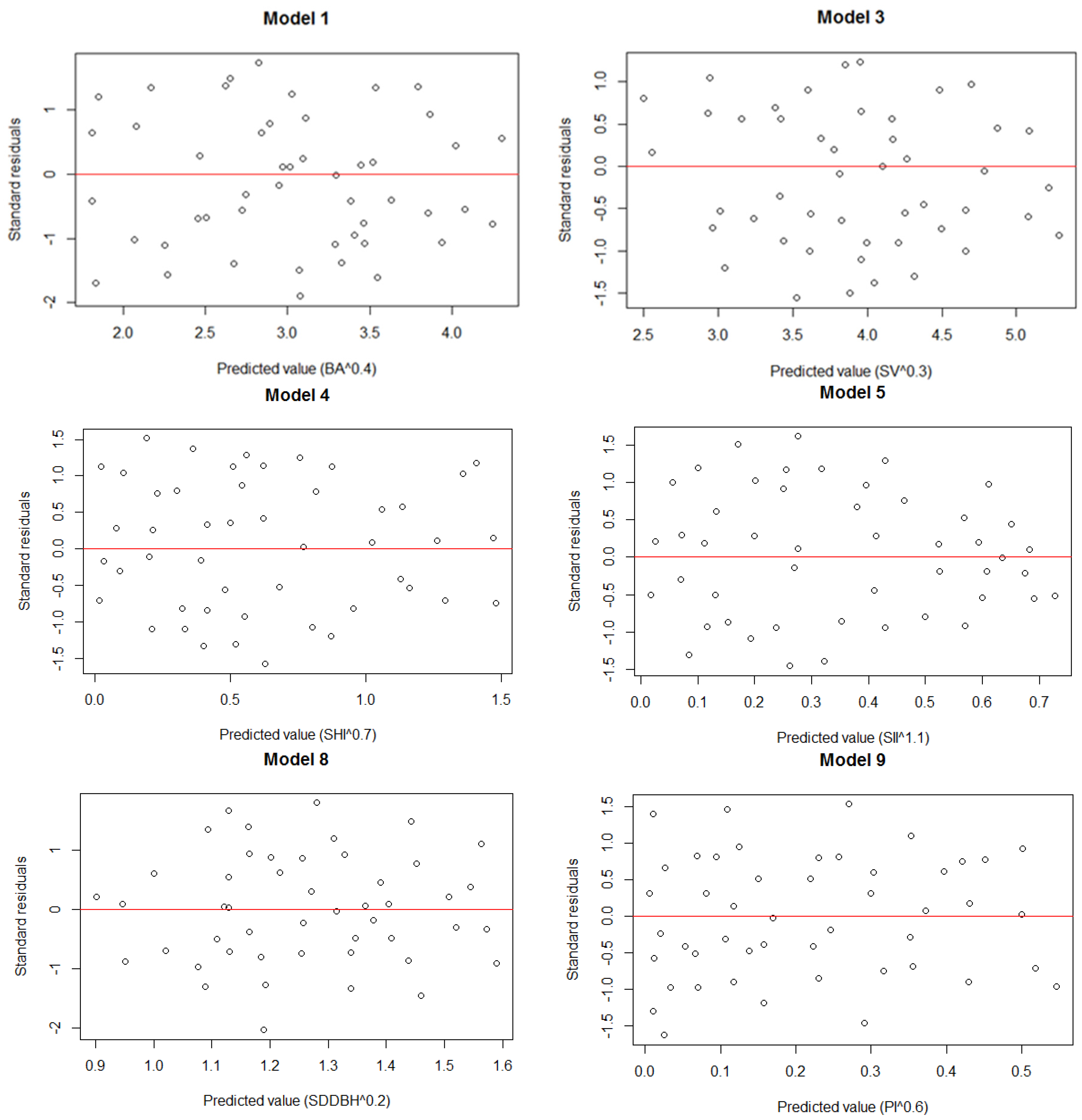
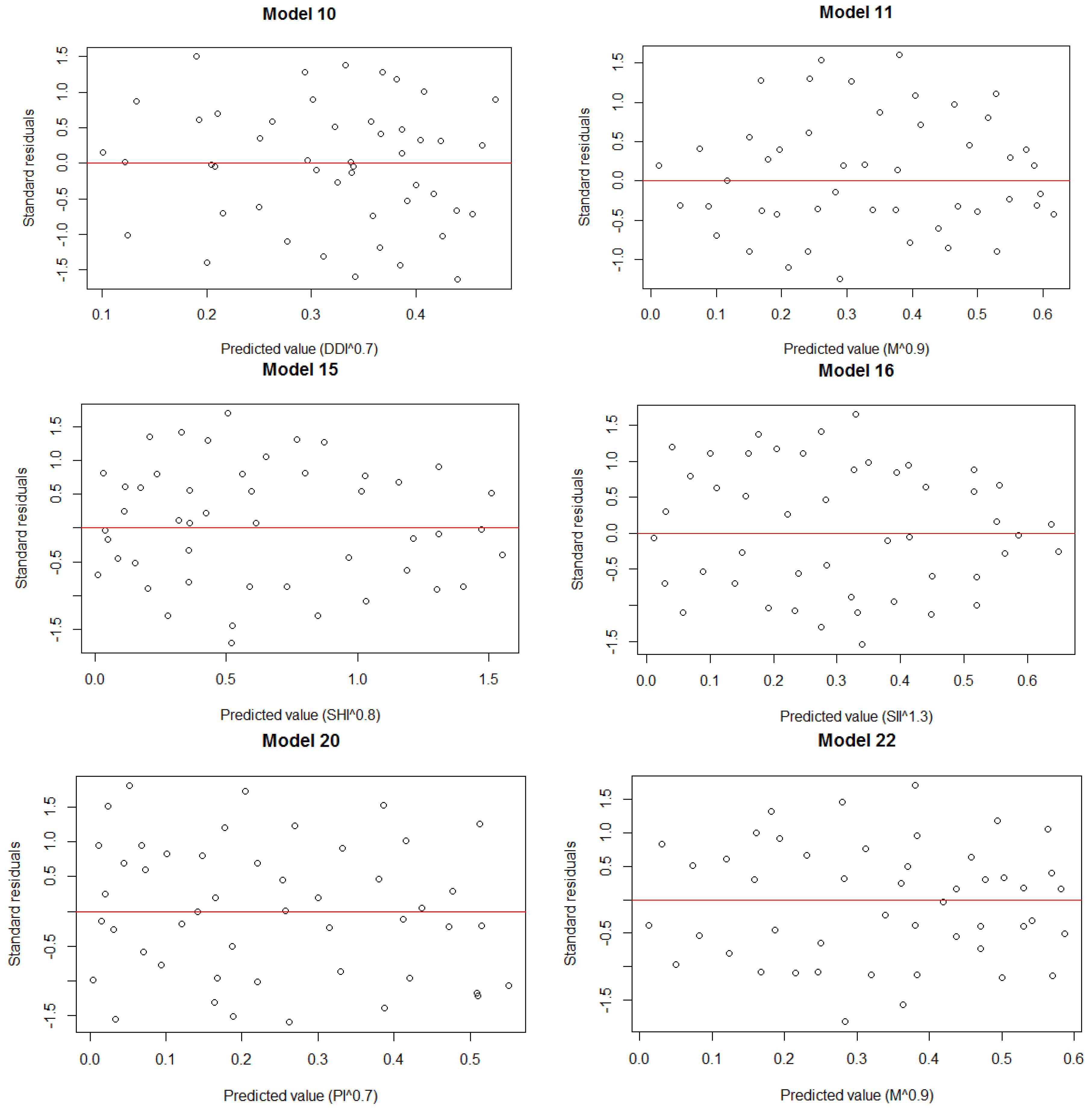
3.3. Model Establishment
| Variables | SDGL _nir | SDGL _red | SDGL _green | SDGL _swir | SDGL _pan | Glcm _ASM | Glcm _contrast | Glcm _correlation | Glcm _dissimilarity | Glcm _entropy | Glcm _homogeneity | Glcm _mean | Glcm _variance |
|---|---|---|---|---|---|---|---|---|---|---|---|---|---|
| NT | 0.245 | −0.156 | 0.124 | 0.270 | −0.152 | 0.110 | −0.391 * | 0.186 | −0.377 * | −0.147 | 0.196 | −0.482 * | −0.419 * |
| QMD | 0.315 | −0.315 | 0.169 | 0.319 * | −0.136 | 0.139 | −0.420 * | 0.095 | −0.419 * | −0.125 | 0.266 | −0.491 * | −0.466 * |
| BA | 0.266 | −0.245 | 0.312 | 0.153 | −0.214 | 0.259 | −0.493 * | 0.149 | −0.507 ** | −0.247 | 0.292 | −0.534 ** | −0.501 ** |
| SV | 0.275 | −0.296 | 0.302 | 0.125 | −0.256 | 0.275 | −0.504 ** | 0.172 | −0.524 ** | −0.270 | 0.280 | −0.559 ** | −0.521 ** |
| GC | 0.396 * | −0.268 | −0.189 | 0.290 | −0.310 | 0.213 | −0.446 * | 0.320 * | −0.510 ** | −0.197 | 0.211 | −0.525 ** | −0.497 * |
| DDI | 0.466 * | −0.398 * | −0.397 * | 0.313 | −0.362 * | 0.376 * | −0.513 ** | 0.442 * | −0.513 ** | −0.400 * | 0.460 * | −0.505 ** | −0.497 * |
| SDDBH | 0.456 * | −0.426 * | −0.208 | 0.336 * | −0.328 * | 0.209 | −0.535 ** | 0.362 * | −0.532 ** | −0.232 | 0.254 | −0.542 ** | −0.513 ** |
| SHI | 0.250 | −0.362 * | −0.262 | 0.064 | −0.208 | 0.349 * | −0.722 ** | 0.511 ** | −0.719 ** | −0.379 * | 0.392 * | −0.812 ** | −0.726 ** |
| SII | 0.231 | −0.381 * | −0.316 * | 0.035 | −0.240 | 0.368 * | −0.690 ** | 0.496 * | −0.698 ** | −0.393 * | 0.378 * | −0.764 ** | −0.697 ** |
| PI | 0.261 | −0.408 * | −0.306 | 0.091 | −0.228 | 0.383 * | −0.694 ** | 0.491 * | −0.709 ** | −0.426 * | 0.412 * | −0.776 ** | −0.697 ** |
| 0.284 | −0.456 * | −0.385 * | 0.066 | −0.270 | 0.397 * | −0.676 ** | 0.534 ** | −0.704 ** | −0.421 * | 0.382 * | −0.759 ** | −0.676 ** | |
| 0.261 | −0.060 | −0.098 | 0.208 | 0.004 | 0.136 | −0.118 | −0.032 | −0.138 | −0.129 | 0.151 | −0.111 | −0.116 | |
| 0.138 | −0.112 | −0.123 | 0.181 | −0.146 | 0.013 | −0.102 | 0.250 | −0.1152 | −0.058 | 0.057 | −0.130 | −0.109 |
| Forest Stand Variables | Predictive Model | RMSE | p | |
|---|---|---|---|---|
| Basal area (BA) | Model 1: BA ^0.4 = −0.023894·Brightness + 2.416160·Max_diff + 4.281999 | 0.52 | 0.856 | 9.837 × 10⁻⁸ |
| Quadratic mean diameter (QMD) | Model 2: QMD^(−0.3) = 0.0010350·Brightness − 0.1741902·Max_diff + 0.4416836 | 0.32 | 0.033 | 4.856 × 10⁻⁵ |
| Stand volume (SV) | Model 3: SV^0.3 = 3.59910 − 0.0157·Brightness +3.45959·Max_diff | 0.50 | 2.217 | 3.154 × 10⁻⁷ |
| Shannon–Wiener index (SHI) | Model 4: SHI^0.7 = −0.026641·mean_red + 3.060631 | 0.62 | 0.309 | 2.854 × 10⁻⁸ |
| Simpson’s index (SII) | Model 5: SII^1.1 = −0.01513·mean_red + 1.70493 | 0.60 | 0.182 | 8.735 × 10⁻⁸ |
| Gini coefficient (GC) | Model 6: GC = 0.334589 − 0.001584·mean_red | 0.42 | 0.046 | 4.643 × 10⁻⁶ |
| Number of trees (NT) | Model 7: NT^0.6 = 107.9658 − 0.4471·Brightness + 14.0616·Max_diff | 0.21 | 21.322 | 4.789 × 10⁻⁶ |
| Standard deviation of DBHs (SDDBH) | Model 8: SDDBH^0.2 = −0.007714·Brightness + 0.021443·SDGL_nir + 1.929803 | 0.51 | 0.125 | 2.849 × 10⁻⁶ |
| Pielou index (PI) | Model 9: PI^0.6 = 3.2225·VI − 4.1580 | 0.60 | 0.136 | 6.676 × 10⁻⁸ |
| Diameter differentiation index (DDI) | Model 10: DDI^0.7 = 0.8917·VI − 0.0118·SDGL_nir − 0.0382·SDGL_green − 0.8697 | 0.57 | 0.067 | 4.17 × 10⁻⁶ |
| Species intermingling index () | Model 11: ^0.9 = 4.5530·VI − 5.9967 | 0.68 | 0.149 | 2.697 × 10⁻⁹ |
| Species intermingling index () | Model 12: ^0.9 = −4.8341 + 3.7593·VI | 0.70 | 0.128 | 3.942 × 10⁻⁶ |

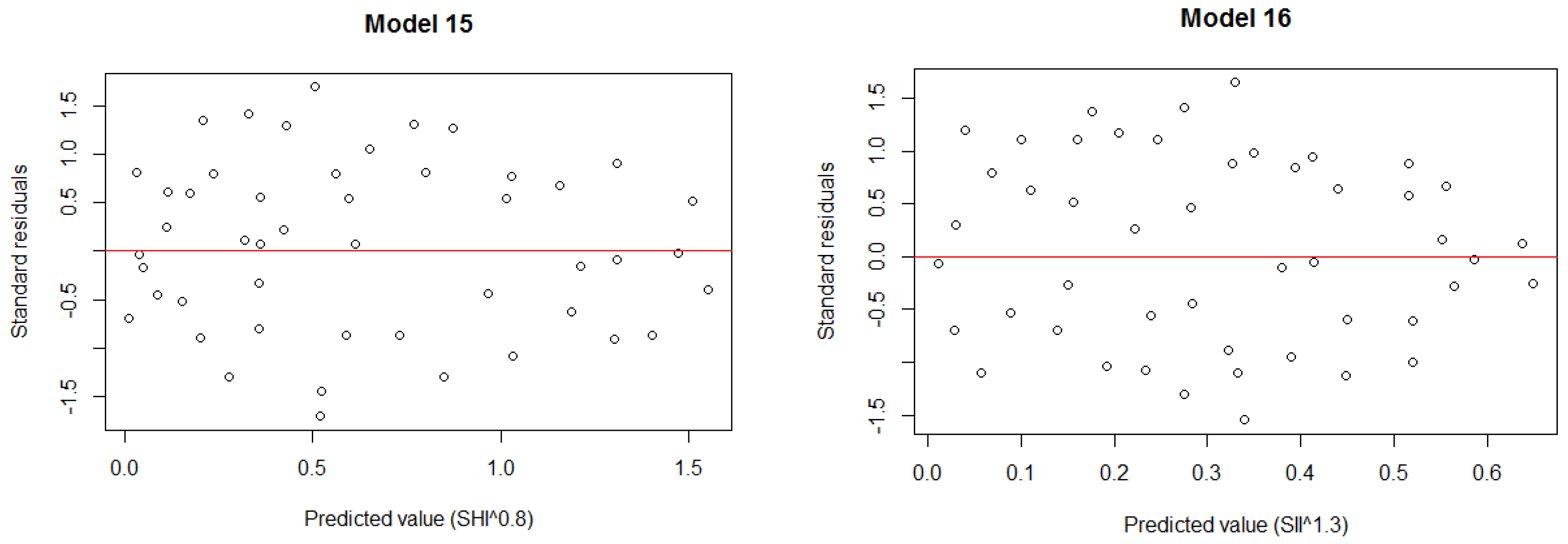
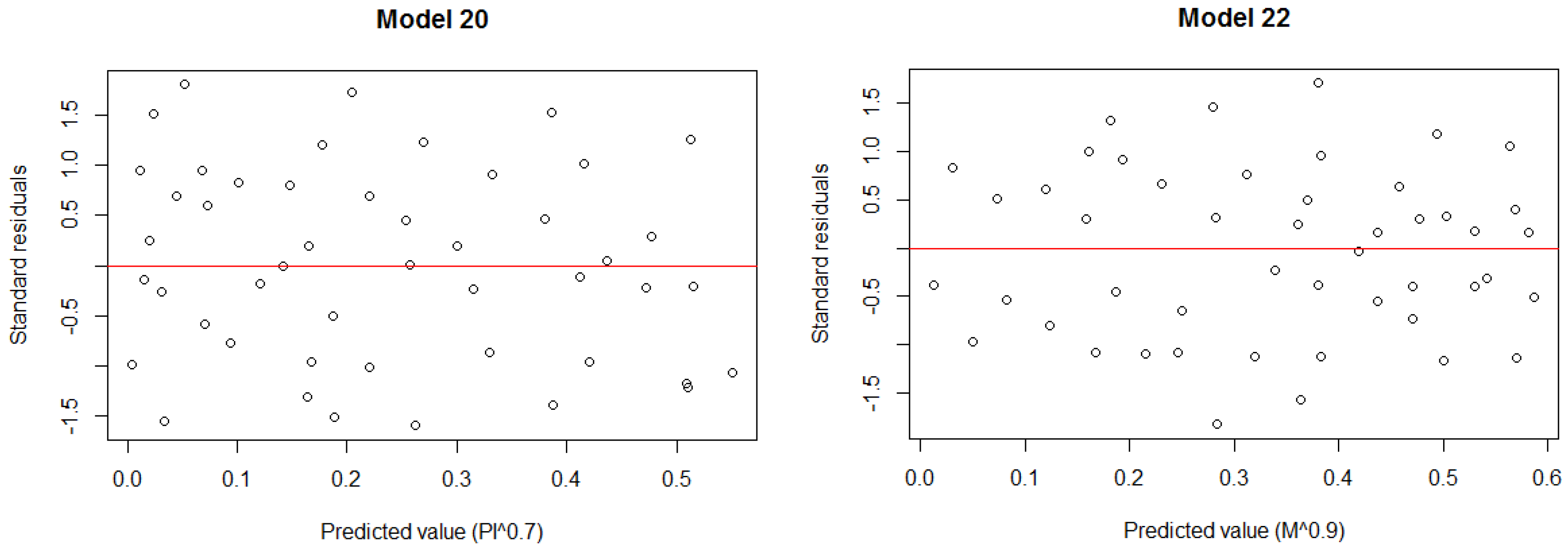
| Forest Stand Variables | Predictive Model | RMSE | p | |
|---|---|---|---|---|
| Basal area (BA) | Model 13: BA^0.4 = −0.08251·Glcm_mean + 4.70834 | 0.38 | 0.951 | 3.68 × 10⁻⁸ |
| Quadratic mean diameter (QMD) | Model 14: QMD^(−0.3) = 0.340853 −0.00698·Glcm_mean | 0.23 | 0.127 | 4.466 × 10⁻⁵ |
| Stand volume (SV) | Model 15: SV^0.3 = −0.09075·Glcm_mean + 5.65686 | 0.40 | 2.601 | 5.475 × 10⁻⁶ |
| Shannon–Wiener index (SHI) | Model 16: SHI^0.8 = −0.11179·Glcm_mean + 3.38682 | 0.62 | 0.321 | 3.357 × 10⁻⁸ |
| Simpson’s index (SII) | Model 17: SII^1.3= −0.058316·Glcm_mean + 1.741997 | 0.59 | 0.169 | 1.219 × 10⁻⁷ |
| Gini coefficient (GC) | Model 18: GC = 0.3508 − 0.006322·Glcm_mean | 0.40 | 0.052 | 0.547 × 10⁻⁶ |
| Number of trees (NT) | Model 19: NT^0.6 = 101.5011 − 1.4812·Glcm_mean | 0.22 | 20.214 | 0.459 × 10⁻⁷ |
| Standard deviation of DBHs (SDDBH) | Model 20: SDDBH^0.2 = −0.0352·Glcm_mean + 2.8799 | 0.28 | 0.200 | 0.0008232 |
| Pielou index (PI) | Model 21: PI^0.7 = −0.041014·Glcm_mean + 1.248652 | 0.57 | 0.127 | 1.964 × 10⁻⁷ |
| Diameter differentiation index (DDI) | Model 22: DDI^0.8 = −0.529751·Glcm_entropy − 0.012799·Glcm_mean − 2.536325·Glcm_ASM + 2.1938 | 0.41 | 0.067 | 0.0003796 |
| Species intermingling index () | Model 23: ^0.9 = −0.28447·Glcm_entropy − 0.04386·Glcm_mean + 1.94016 | 0.59 | 0.160 | 5.475 × 10⁻⁷ |
| Species intermingling index () | Model 24: ^0.9 = 1.577187 − 0.185160·Entropy − 0.034526·Glcm_mean | 0.62 | 0.147 | 3.235 × 10⁻⁶ |


4. Discussion
5. Conclusions
Acknowledgments
Author Contributions
Conflicts of Interest
References
- Eckert, S. Improved forest biomass and carbon estimations using texture measures from WorldView-2 satellite data. Remote Sens. 2012, 4, 810–829. [Google Scholar] [CrossRef]
- Meng, J.; Lu, Y.; Zeng, J. Transformation of a degraded pinus massoniana plantation into a mixed-species irregular forest: Impacts on stand structure and growth in southern China. Forests 2014, 5, 3199–3221. [Google Scholar] [CrossRef]
- Gärtner, S.; Reif, A. The impact of forest transformation on stand structure and ground vegetation in the southern black forest, germany. Plant Soil 2004, 264, 35–51. [Google Scholar] [CrossRef]
- Chauvat, M.; Titsch, D.; Zaytsev, A.S.; Wolters, V. Changes in soil faunal assemblages during conversion from pure to mixed forest stands. For. Ecol. Manag. 2011, 262, 317–324. [Google Scholar] [CrossRef]
- O’Hara, K.L. The silviculture of transformation—A commentary. For. Ecol. Manag. 2001, 151, 81–86. [Google Scholar] [CrossRef]
- Buongiorno, J. Quantifying the implications of transformation from even to uneven-aged forest stands. For. Ecol. Manag. 2001, 151, 121–132. [Google Scholar] [CrossRef]
- Fürstenau, C.; Badeck, F.W.; Lasch, P.; Lexer, M.J.; Lindner, M.; Mohr, P.; Suckow, F. Multiple-use forest management in consideration of climate change and the interests of stakeholder groups. Eur. J. For. Res. 2007, 126, 225–239. [Google Scholar] [CrossRef]
- Puettmann, K.J.; Wilson, S.M.; Baker, S.C.; Donoso, P.J.; Drössler, L.; Amente, G.; Harvey, B.D.; Knoke, T.; Lu, Y.; Nocentini, S. Silvicultural alternatives to conventional even-aged forest management-what limits global adoption? For. Ecosyst. 2015, 2, 1–16. [Google Scholar] [CrossRef]
- Messier, C.; Puettmann, K.J.; Coates, K.D. Managing Forests as Complex Adaptive Systems: Building Resilience to the Challenge of Global Change; Routledge: London, UK, 2013. [Google Scholar]
- Filotas, E.; Parrott, L.; Burton, P.J.; Chazdon, R.L.; Coates, K.D.; Coll, L.; Haeussler, S.; Martin, K.; Nocentini, S.; Puettmann, K.J. Viewing forests through the lens of complex systems science. Ecosphere 2014, 5, 1–23. [Google Scholar] [CrossRef]
- Warfield, J.N. An Introduction to Systems Science; World Scientific Publishing Co., Inc.: Hackensack, NJ, USA, 2006. [Google Scholar]
- Corona, P. Consolidating new paradigms in large-scale monitoring and assessment of forest ecosystems. Environ. Res. 2016, 144, 8–14. [Google Scholar] [CrossRef] [PubMed]
- Ozdemir, I.; Karnieli, A. Predicting forest structural parameters using the image texture derived from worldview-2 multispectral imagery in a dryland forest, israel. Int. J. Appl. Earth Obs. Geoinform. 2011, 13, 701–710. [Google Scholar] [CrossRef]
- Pommerening, A. Approaches to quantifying forest structures. Forestry 2002, 75, 305–324. [Google Scholar] [CrossRef]
- Lexerød, N.L.; Eid, T. An evaluation of different diameter diversity indices based on criteria related to forest management planning. For. Ecol. Manag. 2006, 222, 17–28. [Google Scholar] [CrossRef]
- O’Hara, K. Multiaged Silviculture: Managing for Complex Forest Stand Structures; Oxford University Press: Oxford, UK, 2014. [Google Scholar]
- Bettinger, P.; Tang, M. Tree-level harvest optimization for structure-based forest management based on the species mingling index. Forests 2015, 6, 1121–1144. [Google Scholar] [CrossRef]
- Lei, X.; Tang, M.; Lu, Y.; Hong, L.; Tian, D. Forest inventory in China: Status and challenges. Int. For. Rev. 2009, 11, 52–63. [Google Scholar] [CrossRef]
- Corona, P.; Chirici, G.; McRoberts, R.E.; Winter, S.; Barbati, A. Contribution of large-scale forest inventories to biodiversity assessment and monitoring. For. Ecol. Manag. 2011, 262, 2061–2069. [Google Scholar] [CrossRef]
- Corona, P.; Marchetti, M. Outlining multi-purpose forest inventories to assess the ecosystem approach in forestry. Plant Biosyst. 2007, 141, 243–251. [Google Scholar] [CrossRef]
- Winter, S.; Chirici, G.; McRoberts, R.E.; Hauk, E. Possibilities for harmonizing national forest inventory data for use in forest biodiversity assessments. Forestry 2008, 81, 33–44. [Google Scholar] [CrossRef]
- Gómez, C.; Wulder, M.A.; Montes, F.; Delgado, J.A. Modeling forest structural parameters in the mediterranean pines of central spain using QuickBird-2 imagery and classification and regression tree analysis (CART). Remote Sens. 2012, 4, 135–159. [Google Scholar] [CrossRef]
- Tanaka, S.; Takahashi, T.; Nishizono, T.; Kitahara, F.; Saito, H.; Iehara, T.; Kodani, E.; Awaya, Y. Stand volume estimation using the k-NN technique combined with forest inventory data, satellite image data and additional feature variables. Remote Sens. 2014, 7, 378–394. [Google Scholar] [CrossRef]
- McRoberts, R.E.; Tomppo, E.O. Remote sensing support for national forest inventories. Remote Sens. Environ. 2007, 110, 412–419. [Google Scholar] [CrossRef]
- Wolter, P.T.; Townsend, P.A.; Sturtevant, B.R. Estimation of forest structural parameters using 5 and 10 m SPOT-5 satellite data. Remote Sens. Environ. 2009, 113, 2019–2036. [Google Scholar] [CrossRef]
- Popescu, S.C.; Wynne, R.H.; Nelson, R.F. Measuring individual tree crown diameter with LiDAR and assessing its influence on estimating forest volume and biomass. Can. J. Remote Sens. 2003, 29, 564–577. [Google Scholar] [CrossRef]
- Tsui, O.W.; Coops, N.C.; Wulder, M.A.; Marshall, P.L.; McCardle, A. Using multi-frequency radar and discrete-return LiDAR measurements to estimate above-ground biomass and biomass components in a coastal temperate forest. ISPRS J. Photogramm. Remote Sens. 2012, 69, 121–133. [Google Scholar] [CrossRef]
- Meyer, V.; Saatchi, S.; Poulsen, J.; Clark, C.; Lewis, S.; White, L. LiDAR estimation of aboveground biomass in a tropical coastal forest of gabon. AGU Fall Meet. Abstr. 2012, 1, 0440. [Google Scholar]
- Suárez, J.C.; Ontiveros, C.; Smith, S.; Snape, S. Use of airborne LiDAR and aerial photography in the estimation of individual tree heights in forestry. Comput. Geosci. 2005, 31, 253–262. [Google Scholar] [CrossRef]
- Kwak, D.-A.; Lee, W.-K.; Lee, J.-H.; Biging, G.S.; Gong, P. Detection of individual trees and estimation of tree height using LiDAR data. J. For. Res. 2007, 12, 425–434. [Google Scholar] [CrossRef]
- Unger, D.R.; Hung, I.-K.; Brooks, R.; Williams, H. Estimating number of trees, tree height and crown width using LiDAR data. GISci. Remote Sens. 2014, 51, 227–238. [Google Scholar] [CrossRef]
- Koch, B.; Heyder, U.; Weinacker, H. Detection of individual tree crowns in airborne LiDAR data. Photogramm. Eng. Remote Sens. 2006, 72, 357–363. [Google Scholar] [CrossRef]
- Jing, L.; Hu, B.; Li, J.; Noland, T. Automated delineation of individual tree crowns from LiDAR data by multi-scale analysis and segmentation. Photogramm. Eng. Remote Sens. 2012, 78, 1275–1284. [Google Scholar] [CrossRef]
- Chang, A.; Eo, Y.; Kim, Y.; Kim, Y. Identification of individual tree crowns from LiDAR data using a circle fitting algorithm with local maxima and minima filtering. Remote Sens. Lett. 2013, 4, 29–37. [Google Scholar] [CrossRef]
- Castillo-Santiago, M.A.; Ricker, M.; de Jong, B.H. Estimation of tropical forest structure from spot-5 satellite images. Int. J. Remote Sens. 2010, 31, 2767–2782. [Google Scholar] [CrossRef]
- Magurran, A.E. Measuring Biological Diversity; John Wiley & Sons: New York, NY, USA, 2013. [Google Scholar]
- Li, Y.; Hui, G.; Zhao, Z.; Hu, Y. The bivariate distribution characteristics of spatial structure in natural korean pine broad-leaved forest. J. Veg. Sci. 2012, 23, 1180–1190. [Google Scholar] [CrossRef]
- Hui, G.; Kv, G.; Hu, Y.; Chen, B. Characterizing forest spatial distribution pattern with the mean value of uniform angle index. Acta Ecol. Sin. 2003, 24, 1225–1229. [Google Scholar]
- Gangying, H.; von Gadow, K.; Albert, M. The neighbourhood pattern—A new structure parameter for describing distribution of forest tree position. Sci. Silvae Sin. 1999, 35, 37–42. [Google Scholar]
- Yan-bo, H.; Gang-ying, H. A discussion on forest management method optimizing forest spatial structure. For. Res. 2006, 19, 1–4. [Google Scholar]
- Gangying, H.; Li, L.; Zhonghua, Z.; Puxing, D. Comparison of methods in analysis of the tree spatial distribution pattern. Acta Ecol. Sin. 2007, 27, 4717–4728. [Google Scholar] [CrossRef]
- Pommerening, A.; Stoyan, D. Edge-correction needs in estimating indices of spatial forest structure. Can. J. For. Res. 2006, 36, 1723–1739. [Google Scholar] [CrossRef]
- Germany, Trimble. eCognition Developer 7 Reference Book; Trimble Germany: Munich, Germany, 2011. [Google Scholar]
- Rouse, J.W., Jr.; Haas, R.; Schell, J.; Deering, D. Monitoring vegetation systems in the great plains with ERTS. In Third Earth Resources Technology Satellite-1 Symposium- Volume I: Technical Presentations; NASA SP-351; NASA: Washington, DC, USA, 1974; p. 309. [Google Scholar]
- Jordan, C.F. Derivation of leaf-area index from quality of light on the forest floor. Ecology 1969, 50, 663–666. [Google Scholar] [CrossRef]
- Lyon, J.G.; Yuan, D.; Lunetta, R.S.; Elvidge, C.D. A change detection experiment using vegetation indices. Photogramm. Eng. Remote Sens. 1998, 64, 143–150. [Google Scholar]
- Kanemasu, E. Seasonal canopy reflectance patterns of wheat, sorghum, and soybean. Remote Sens. Environ. 1974, 3, 43–47. [Google Scholar] [CrossRef]
- Huete, A.R. A soil-adjusted vegetation index (SAVI). Remote Sens. Environ. 1988, 25, 295–309. [Google Scholar] [CrossRef]
- Verstraete, M.M.; Pinty, B. Designing optimal spectral indexes for remote sensing applications. IEEE Trans. Geosci. Remote Sens. 1996, 34, 1254–1265. [Google Scholar] [CrossRef]
- Ouma, Y.O.; Ngigi, T.; Tateishi, R. On the optimization and selection of wavelet texture for feature extraction from high-resolution satellite imagery with application towards urban-tree delineation. Int. J. Remote Sens. 2006, 27, 73–104. [Google Scholar] [CrossRef]
- Song, C.; Dickinson, M.B.; Su, L.; Zhang, S.; Yaussey, D. Estimating average tree crown size using spatial information from ikonos and quickbird images: Across-sensor and across-site comparisons. Remote Sens. Environ. 2010, 114, 1099–1107. [Google Scholar] [CrossRef]
- Gebreslasie, M.; Ahmed, F.; van Aardt, J.A. Extracting structural attributes from IKONOS imagery for eucalyptus plantation forests in Kwazulu-Natal, South Africa, using image texture analysis and artificial neural networks. Int. J. Remote Sens. 2011, 32, 7677–7701. [Google Scholar] [CrossRef]
- Shaban, M.; Dikshit, O. Improvement of classification in urban areas by the use of textural features: The case study of Lucknow City, Uttar Pradesh. Int. J. Remote Sens. 2001, 22, 565–593. [Google Scholar] [CrossRef]
- Sheather, S. A Modern Approach to Regression with R; Springer: Berlin, Germany, 2009. [Google Scholar]
- Wallner, A.; Elatawneh, A.; Schneider, T.; Knoke, T. Estimation of forest structural information using rapideye satellite data. Forestry 2015, 88, 96–107. [Google Scholar] [CrossRef]
- State Forestry Administration of the People’s Republic of China. The 8th forest resources inventory results. For. Res. Manag. 2014, 1, 1–2. [Google Scholar]
- Jensen, J.R. Introductory Digital Image Processing: A Remote Sensing Perspective; Pearson College Division: Englewood Cliff, NJ, USA, 2005. [Google Scholar]
- Steininger, M. Satellite estimation of tropical secondary forest above-ground biomass: Data from Brazil and Bolivia. Int. J. Remote Sens. 2000, 21, 1139–1157. [Google Scholar] [CrossRef]
- Eckert, S. A Contribution to Sustainable Forest Management in Patagonia: Object-Oriented Classification and Forest Parameter Extraction Based on Aster and Ladsat ETM+ Data; Remote Sensing Laboratories, Department of Geography, University of Zurich: Zurich, Switzerland, 2006. [Google Scholar]
- Wulder, M.A.; LeDrew, E.F.; Franklin, S.E.; Lavigne, M.B. Aerial image texture information in the estimation of northern deciduous and mixed wood forest leaf area index (LAI). Remote Sens. Environ. 1998, 64, 64–76. [Google Scholar] [CrossRef]
- Kim, M.; Madden, M.; Warner, T.A. Forest type mapping using object-specific texture measures from multispectral Ikonos imagery. Photogramm. Eng. Remote Sens. 2009, 75, 819–829. [Google Scholar] [CrossRef]
- Lu, D.; Weng, Q. A survey of image classification methods and techniques for improving classification performance. Int. J. Remote Sens. 2007, 28, 823–870. [Google Scholar] [CrossRef]
- Franklin, S.; Wulder, M.; Gerylo, G. Texture analysis of IKONOS panchromatic data for Douglas-fir forest age class separability in British Columbia. Int. J. Remote Sens. 2001, 22, 2627–2632. [Google Scholar] [CrossRef]
- Li, Y.; Hui, G.; Zhao, Z.; Hu, Y.; Ye, S. Spatial structural characteristics of three hardwood species in Korean pine broad-leaved forest—Validating the bivariate distribution of structural parameters from the point of tree population. For. Ecol. Manag. 2014, 314, 17–25. [Google Scholar] [CrossRef]
- Ota, T.; Mizoue, N.; Yoshida, S. Influence of using texture information in remote sensed data on the accuracy of forest type classification at different levels of spatial resolution. J. For. Res. 2011, 16, 432–437. [Google Scholar] [CrossRef]
- Franklin, S.; Hall, R.; Moskal, L.; Maudie, A.; Lavigne, M. Incorporating texture into classification of forest species composition from airborne multispectral images. Int. J. Remote Sens. 2000, 21, 61–79. [Google Scholar] [CrossRef]
- Kayitakire, F.; Giot, P.; Defourny, P. Automated delineation of the forest stands using digital color orthophotos: Case study in Belgium. Can. J. Remote Sens. 2002, 28, 629–640. [Google Scholar] [CrossRef]
- Nagendra, H.; Rocchini, D.; Ghate, R.; Sharma, B.; Pareeth, S. Assessing plant diversity in a dry tropical forest: Comparing the utility of landsat and ikonos satellite images. Remote Sens. 2010, 2, 478–496. [Google Scholar] [CrossRef]
- St-Louis, V.; Pidgeon, A.M.; Radeloff, V.C.; Hawbaker, T.J.; Clayton, M.K. High-resolution image texture as a predictor of bird species richness. Remote Sens. Environ. 2006, 105, 299–312. [Google Scholar] [CrossRef]
- Wood, E.M.; Pidgeon, A.M.; Radeloff, V.C.; Keuler, N.S. Image texture predicts avian density and species richness. PLoS ONE 2013, 8, e63211. [Google Scholar]
- Newton, A.C. Forest Ecology and Conservation: A Handbook of Techniques; Oxford University Press: Oxford, UK, 2007. [Google Scholar]
- Schneider, D.C. Quantitative Ecology: Measurement, Models and Scaling; Academic Press: Cambridge, MA, USA, 2009. [Google Scholar]
- Gallardo-Cruz, J.A.; Meave, J.A.; González, E.J.; Lebrija-Trejos, E.E.; Romero-Romero, M.A.; Pérez-García, E.A.; Gallardo-Cruz, R.; Hernández-Stefanoni, J.L.; Martorell, C. Predicting tropical dry forest successional attributes from space: Is the key hidden in image texture? PLoS ONE 2012, 7, e30506–e30512. [Google Scholar] [CrossRef] [PubMed]
- Couteron, P.; Pelissier, R.; Nicolini, E.A.; Paget, D. Predicting tropical forest stand structure parameters from fourier transform of very high-resolution remotely sensed canopy images. J. Appl. Ecol. 2005, 42, 1121–1128. [Google Scholar] [CrossRef]
- Mora, B.; Wulder, M.A.; White, J.C.; Hobart, G. Modeling stand height, volume, and biomass from very high spatial resolution satellite imagery and samples of airborne LiDAR. Remote Sens. 2013, 5, 2308–2326. [Google Scholar] [CrossRef]
- Ozdemir, I.; Norton, D.A.; Ozkan, U.Y.; Mert, A.; Senturk, O. Estimation of tree size diversity using object oriented texture analysis and aster imagery. Sensors 2008, 8, 4709–4724. [Google Scholar] [CrossRef]
- Lamonaca, A.; Corona, P.; Barbati, A. Exploring forest structural complexity by multi-scale segmentation of VHR imagery. Remote Sens. Environ. 2008, 112, 2839–2849. [Google Scholar] [CrossRef]
- Parrott, L. Complexity and the limits of ecological engineering. Trans. Am. Soc. Agric. Eng. 2002, 45, 1697–1702. [Google Scholar] [CrossRef]
- He, F.; Duncan, R.P. Density-dependent effects on tree survival in an old-growth Douglas fir forest. J. Ecol. 2000, 88, 676–688. [Google Scholar] [CrossRef]
- Getzin, S.; Dean, C.; He, F.; Trofymow, J.A.; Wiegand, K.; Wiegand, T. Spatial patterns and competition of tree species in a Douglas-fir chronosequence on vancouver island. Ecography 2006, 29, 671–682. [Google Scholar] [CrossRef]
- Hao, Z.; Zhang, J.; Song, B.; Ye, J.; Li, B. Vertical structure and spatial associations of dominant tree species in an old-growth temperate forest. For. Ecol. Manag. 2007, 252, 1–11. [Google Scholar] [CrossRef]
- Sánchez-González, M.; del Río, M.; Cañellas, I.; Montero, G. Distance independent tree diameter growth model for cork oak stands. For. Ecol. Manag. 2006, 225, 262–270. [Google Scholar] [CrossRef]
- Condés, S.; Sterba, H. Comparing an individual tree growth model for pinus halepensis mill. In the Spanish region of murcia with yield tables gained from the same area. European J. For. Res. 2008, 127, 253–261. [Google Scholar] [CrossRef]
- Zhao, D.; Borders, B.; Wilson, M. Individual-tree diameter growth and mortality models for bottomland mixed-species hardwood stands in the lower mississippi alluvial valley. For. Ecol. Manag. 2004, 199, 307–322. [Google Scholar] [CrossRef]
- Pukkala, T.; Lähde, E.; Laiho, O. Growth and yield models for uneven-sized forest stands in Finland. For. Ecol. Manag. 2009, 258, 207–216. [Google Scholar] [CrossRef]
- Kayitakire, F.; Hamel, C.; Defourny, P. Retrieving forest structure variables based on image texture analysis and IKONOS-2 imagery. Remote Sens. Environ. 2006, 102, 390–401. [Google Scholar] [CrossRef]
- Andersen, H.-E.; McGaughey, R.J.; Reutebuch, S.E. Estimating forest canopy fuel parameters using LiDAR data. Remote Sens. Environ. 2005, 94, 441–449. [Google Scholar] [CrossRef]
- Dye, M.; Mutanga, O.; Ismail, R. Combining spectral and textural remote sensing variables using random forests: Predicting the age of pinus patula forests in Kwazulu-Natal, South Africa. J. Spat. Sci. 2012, 57, 193–211. [Google Scholar] [CrossRef]
- Lottering, R.; Mutanga, O. Estimating the road edge effect on adjacent eucalyptus grandis forests in Kwazulu-Natal, South Africa, using texture measures and an artificial neural network. J. Spat. Sci. 2012, 57, 153–173. [Google Scholar] [CrossRef]
- Jensen, J.; Qiu, F.; Ji, M. Predictive modelling of coniferous forest age using statistical and artificial neural network approaches applied to remote sensor data. Int. J. Remote Sens. 1999, 20, 2805–2822. [Google Scholar]
- Ingram, J.C.; Dawson, T.P.; Whittaker, R.J. Mapping tropical forest structure in southeastern Madagascar using remote sensing and artificial neural networks. Remote Sens. Environ. 2005, 94, 491–507. [Google Scholar] [CrossRef]
- Lobell, D.B.; Ortiz-Monasterio, J.I.; Asner, G.P.; Naylor, R.L.; Falcon, W.P. Combining field surveys, remote sensing, and regression trees to understand yield variations in an irrigated wheat landscape. Agron. J. 2005, 97, 241–249. [Google Scholar]
- Chubey, M.S.; Franklin, S.E.; Wulder, M.A. Object-based analysis of IKONOS-2 imagery for extraction of forest inventory parameters. Photogramm. Eng. Remote Sens. 2006, 72, 383–394. [Google Scholar] [CrossRef]
- Yu, X.; Hyyppä, J.; Vastaranta, M.; Holopainen, M.; Viitala, R. Predicting individual tree attributes from airborne laser point clouds based on the random forests technique. ISPRS J. Photogramm. Remote Sens. 2011, 66, 28–37. [Google Scholar] [CrossRef]
- Baccini, A.; Friedl, M.; Woodcock, C.; Warbington, R. Forest biomass estimation over regional scales using multisource data. Geophys. Res. Lett. 2004, 31. [Google Scholar] [CrossRef]
- De’ath, G.; Fabricius, K.E. Classification and regression trees: A powerful yet simple technique for ecological data analysis. Ecology 2000, 81, 3178–3192. [Google Scholar] [CrossRef]
- Breiman, L. Random forests. Mach. Learn. 2001, 45, 5–32. [Google Scholar] [CrossRef]
- Elith, J.; Leathwick, J.R.; Hastie, T. A working guide to boosted regression trees. J. Anim. Ecol. 2008, 77, 802–813. [Google Scholar] [CrossRef] [PubMed]
- Krause, P.; Boyle, D.; Bäse, F. Comparison of different efficiency criteria for hydrological model assessment. Adv. Geosci. 2005, 5, 89–97. [Google Scholar] [CrossRef]
- Nash, J.; Sutcliffe, J.V. River flow forecasting through conceptual models part I—A discussion of principles. J. Hydrol. 1970, 10, 282–290. [Google Scholar] [CrossRef]
- Janssen, P.; Heuberger, P. Calibration of process-oriented models. Ecol. Model. 1995, 83, 55–66. [Google Scholar] [CrossRef]
- Harmer, R.; Kiewitt, A.; Morgan, G. Effects of overstorey retention on ash regeneration and bramble growth during conversion of a pine plantation to native broadleaved woodland. Eur. J. For. Res. 2012, 131, 1833–1843. [Google Scholar] [CrossRef]
© 2016 by the authors; licensee MDPI, Basel, Switzerland. This article is an open access article distributed under the terms and conditions of the Creative Commons by Attribution (CC-BY) license (http://creativecommons.org/licenses/by/4.0/).
Share and Cite
Meng, J.; Li, S.; Wang, W.; Liu, Q.; Xie, S.; Ma, W. Estimation of Forest Structural Diversity Using the Spectral and Textural Information Derived from SPOT-5 Satellite Images. Remote Sens. 2016, 8, 125. https://doi.org/10.3390/rs8020125
Meng J, Li S, Wang W, Liu Q, Xie S, Ma W. Estimation of Forest Structural Diversity Using the Spectral and Textural Information Derived from SPOT-5 Satellite Images. Remote Sensing. 2016; 8(2):125. https://doi.org/10.3390/rs8020125
Chicago/Turabian StyleMeng, Jinghui, Shiming Li, Wei Wang, Qingwang Liu, Shiqin Xie, and Wu Ma. 2016. "Estimation of Forest Structural Diversity Using the Spectral and Textural Information Derived from SPOT-5 Satellite Images" Remote Sensing 8, no. 2: 125. https://doi.org/10.3390/rs8020125
APA StyleMeng, J., Li, S., Wang, W., Liu, Q., Xie, S., & Ma, W. (2016). Estimation of Forest Structural Diversity Using the Spectral and Textural Information Derived from SPOT-5 Satellite Images. Remote Sensing, 8(2), 125. https://doi.org/10.3390/rs8020125