Article

Evaluating Multi-Sensor Nighttime Earth Observation Data for Identification of Mixed vs. Residential Use in Urban Areas

1
Social, Urban, Rural & Resilience (GSURR), The World Bank, Washington, DC 20006, USA
2
Institute of Engineering, National Autonomous University of Mexico (UNAM), Mexico City 04510, Mexico
*
Author to whom correspondence should be addressed.
These authors contributed equally to this work.
Remote Sens. 2016, 8(2), 114; https://doi.org/10.3390/rs8020114
Submission received: 28 November 2015 / Revised: 13 January 2016 / Accepted: 25 January 2016 / Published: 4 February 2016

Abstract

:
This paper introduces a novel top-down approach to geospatially identify and distinguish areas of mixed use from predominantly residential areas within urban agglomerations. Under the framework of the World Bank’s Central American Country Disaster Risk Profiles (CDRP) initiative, a disaggregated property stock exposure model has been developed as one of the key elements for disaster risk and loss estimation. Global spatial datasets are therefore used consistently to ensure wide-scale applicability and transferability. Residential and mixed use areas need to be identified in order to spatially link accordingly compiled property stock information. In the presented study, multi-sensor nighttime Earth Observation data and derivative products are evaluated as proxies to identify areas of peak human activity. Intense artificial night lighting in that context is associated with a high likelihood of commercial and/or industrial presence. Areas of low light intensity, in turn, can be considered more likely residential. Iterative intensity thresholding is tested for Cuenca City, Ecuador, in order to best match a given reference situation based on cadastral land use data. The results and findings are considered highly relevant for the CDRP initiative, but more generally underline the relevance of remote sensing data for top-down modeling approaches at a wide spatial scale.

Graphical Abstract

1. Introduction

Issues of urban development are increasingly being addressed at the global scale, with international non-governmental organizations (NGOs) and development institutions often setting the path and moving the public agenda forward. Regularly published reports such as the United Nations’ World Urbanization Prospects [1] or the World Bank’s World Development [2] and Global Monitoring Reports [3] address fundamental issues and define key research questions to be tackled by the scientific and international development community. In that context it has become more and more evident that spatial data is playing a crucial role for consistent cross-regional analyses and unbiased evaluation of locally implemented actions. Remote sensing data in particular provide a rich and globally consistent source for analyses at multiple levels. At the global scale, different aspects have to be considered than for local-level spatial analyses, including consistency, scalability, retraceability etc. Several global project initiatives address these issues in various thematic domains. The World Bank’s Global Urban Growth Data Initiative, for example, addresses pending issues of regional definition and data incompatibilities and supports the international collaborative setup and development of a consistent data set of global urban extents and associated population distribution patterns. In the same context, the Global Human Settlement Working Group, established under the umbrella of the Group on Earth Observations (GEO) (www.earthobservations.org/ghs), aims at establishing a new generation of global settlement measurements and products based on consistent high-resolution satellite imagery analysis.
The presented study has been carried out within the framework of the World Bank’s Country Disaster Risk Profiles (CDRP) project initiative which has been successfully implemented at the continental scale for Central America [4] and is currently being expanded to the Caribbean Region. With the clear aim at extending to other regions, global applicability and easy transferability are considered crucial for the model setup. Global spatial datasets are therefore used throughout the CDRP project, with the presented approach specifically developed to support implementation of a disaggregated property stock exposure model, one of the key elements for subsequent disaster risk and loss estimation. While focusing primarily on natural hazards and risks, urban-rural identification and intra-urban classification aspects are highly relevant for setting the basic spatial framework for analysis [5].
This paper introduces a novel approach to geospatially identify and distinguish areas of mixed use from predominantly residential areas within urban agglomerations. After initial urban-rural classification at a 1 km grid level, that urban mask needs to be classified in residential and mixed use areas in order to spatially link accordingly compiled property stock information (e.g., from global tabular databases such as PAGER-STR [6]). The distinct identification of urban residential and mixed use areas serves as crucial input to define inventory regions for subsequent exposure assessment. Impervious Surface Area (ISA) data [7] based on remotely sensed nighttime lights from the Defense Meteorological Satellite Program’s (DMSP) OLS sensor (Operational Linescan System) are used as proxy to identify areas of peak human activity, often associated with a high likelihood of commercial and/or industrial presence. ISA is chosen due to its inherent correlation with built-up area (providing an indication on the percentage of built-up per grid cell) and thus good suitability for building stock related land use classification. Several ISA thresholds are tested for a case study in Cuenca City, Ecuador, in order to best match a given reference situation on the ground, where local-level cadastral land use data is used to identify the actual distribution ratio of residential vs. mixed use areas. Furthermore, unaltered nightlight intensity data as provided by the VIIRS sensor (Visible Infrared Imaging Radiometer Suite) [8] are evaluated as alternative to the ISA data. With the DMSP program fading out VIIRS provides the option for successive nighttime Earth Observation analyses due to its low light imaging capability. We apply the same methodological steps as for the ISA data in order to determine best-matching thresholds for binary land use classification and subsequently perform a comparative analysis of the results. Also scale effects are accounted for in that regard with VIIRS featuring a higher spatial resolution than OLS-based data products.
Preliminary results of this study were presented at the ECRS-1 conference [9]. Extensive further research and integration of alternative data sources then lead to the multi-sensor approach illustrated in this paper, highlighting the relevance of global remote sensing data for top-down modeling approaches at wide spatial scale. Outcome is considered relevant for global urban spatial modeling in a variety of topical domains including urban monitoring, disaster risk management, and regional development.

2. Study Area and Data

Due to availability of detailed in situ reference data for comparative analysis and evaluation of the proposed methodology, the city of Cuenca, Ecuador, was chosen as study area. Cuenca City is located in the mountainous southern region of Ecuador at an elevation of around 2500 m above sea level and is the capital of the Azuay province (Figure 1). The city stretches across an area of roughly 70 km2 and had an urban population of 329,928 inhabitants according to the census 2010. Latest figures of the Ecuador National Statistical Office (INEC) estimate an urban population of approximately 400,000 in 2015.
Figure 1. Study area Cuenca City, Ecuador.
Remotesensing 08 00114 g001
The use of satellite-observed nighttime lights has a long tradition in research dealing with monitoring urban areas and patterns of human and economic activity [10,11,12,13,14,15,16] as well as its impact on the environment [17,18,19]. As opposed to attempts of using nighttime lights for basic delineation of urban areas or as weights for population disaggregation, in this paper we rather aim at exploring the use and value in determining intra-urban characteristics.
Public-domain applications of nighttime Earth Observation have long been restricted to one satellite sensor, namely the Operational Linescan system (OLS) onboard the Defense Meteorological Satellite Program (DMSP) platform [20]. More recently, data from the Visible Infrared Imaging Radiometer Suite (VIIRS) sensor onboard the Suomi NPP satellite platform have become available, providing both higher spatial and radiometric resolution and being considered as natural successor to the fading-out DMSP-OLS series [21]. The commercial satellite EROS-B also offers nighttime acquisition capability, even at very high spatial resolution [22]. However, global-scale and temporally continuous open data availability remains restricted to DMSP-OLS and NPP-VIIRS, therefore the only reasonable choice given the scope of the above-outlined CDRP initiative. In the following, we briefly introduce the two data sources we use for the Cuenca City case study, (1) the Impervious Surface Area (ISA) product derived from DMSP-OLS; and (2) VIIRS Day/Night band light intensity data.

2.1. Impervious Surface Area (ISA) Data, Derived from DMSP-OLS

The OLS sensor onboard the DMSP satellite series is able to detect faint light on the Earth’s surface at night due to its high sensitivity in the visible spectrum. While initially designed to monitor cloud coverage, that low light imaging capacity allows identification of various light emitting sources including human settlements and associated human activity patterns [20]. The National Geophysical Data Center (NGDC) of the National Oceanic and Atmospheric Administration (NOAA) is processing and archiving OLS imagery, thereby also making certain derived products accessible to the public. DMSP-OLS data was first used to approximate impervious surface area (ISA) in the early 2000s in the development of a national-scale model for the conterminous United States [23]. The ISA approach was then consequently adjusted to global scale whereby a radiance-calibrated annual composite of nighttime lights is analyzed in conjunction with ancillary data such as population counts. Output is consistently provided at 30 arc-sec spatial resolution giving indication on the distribution of manmade surfaces including buildings, roads and related elements [7].
Due to its relevance for a broad set of applications, global impervious surface or general built-up area mapping has been in the focus of attention for a while with data from different satellite sensors used and various approaches implemented (overview provided by [24]), recent efforts including high resolution products such as the Global Urban Footprint (GUF) [25] and the Global Human Settlement Layer (GHSL) [26]. The DMSP-derived ISA data set is unique in a sense that it does not directly extract built-up from satellite imagery but uses artificial night lighting as proxy measure. While a detected general correlation between night lights and impervious surfaces provides the basis for the global ISA product, inherent patterns point to different human activities (e.g., commercial, industrial) rather than mere built structures. Given the scope and purpose of the presented study this two-sided relation to built-up with a specific weight on non-residential human activity patterns is particularly relevant. Figure 2 shows the global ISA data set for the year 2010 extracted for the Cuenca City study area.
Figure 2. Impervious Surface Area (ISA)—30 arc-sec grid for Cuenca City.
Remotesensing 08 00114 g002

2.2. VIIRS Day/Night Band Data

Since 2011 the VIIRS sensor onboard the Suomi NPP satellite platform provides a natural successor to DMSP-OLS with its panchromatic Day/Night Band (DNB) detecting dim nighttime scenes in similar manner. Using advanced processing schemes (e.g., excluding/correcting data impacted by stray light), NOAA-NGDC is producing global monthly composite products featuring average radiance values at 15 arc-sec spatial resolution [27]. As supplementary product the number of cloud-free observations that was used to create the average composite is reported for each cell.
In addition to its superior spatial resolution, VIIRS offers a set of improvements over OLS-derived nighttime lights. These include lower light detection limits, improved dynamic range as well as quantification and calibration options previously unavailable [21]. One of the few disadvantages of VIIRS, on the other hand, refers to the later overpass time (after midnight), when outdoor lighting is at a significantly lower level as compared to early evening when OLS acquisitions are made. Figure 3 illustrates the VIIRS DNB data for the June 2015 monthly composite extracted for the Cuenca City study area (left). For comparative purposes, we also aggregate that data to a 30 arc-sec grid (right), thus matching the resolution of the ISA product.

2.3. Cadastral Data

Since 2010 the Municipality of Cuenca has intensified the efforts to collect specific information on all buildings located in the urban area of Cuenca City enabling the construction of a complete cadastral database including geo-localization and information on building characteristics.
Figure 3. VIIRS Day/Night Band (DNB) data for Cuenca City. 15 arc-sec grid (left). Aggregated 30 arc-sec grid (right).
Remotesensing 08 00114 g003
More specifically, this cadastral database contains detailed information on the use of each building, allowing for example the distinction of residential and nonresidential occupancy types. Data sources that served as input for the cadastral data base originate from different national entities such as the Municipality of Cuenca, the National Institute of Statistics and Census (INEC), the Telecommunications, Water and Sewage Service Company of Cuenca (ETAPA), the National Secretariat for Risk Management (SNGR) and the University of Cuenca. After a validation and filtering process, the cadastral building data base eventually comprises 65,436 records [28]. Each building footprint record is georeferenced and includes information on built-up area (in m2) and occupancy type (Figure 4). Residential buildings thereby cover an area of 12.9 km2, complemented by a 4.3 km2 non-residential built-up area.
Figure 4. Cadastral building footprints of Cuenca City, classified in residential and non-residential occupancy types.
Remotesensing 08 00114 g004
For comparative purposes, we aggregate building footprint data to a 15 arc-sec and a 30 arc-sec grid respectively, thus matching the resolutions of the two analyzed nighttime lights data sets. Figure 5 illustrates the aggregated grids for the non-residential share of the built-up area. On top, non-residential built-up percentage is shown. At the bottom, each cell’s contribution to the total built-up area is visualized, whereby a main cluster in the center of the city is clearly depicted.
Figure 5. Cadastral data for Cuenca City aggregated to grids at 15 arc-sec (left) and 30 arc-sec (right) resolution. Non-residential built-up percentage (top). Percent-contribution of each cell to the total non-residential built-up area (bottom).
Remotesensing 08 00114 g005

3. Methods

As outlined in the introduction, the presented study was carried out under the framework of the World Bank’s Central American Country Disaster Risk Profiles (CDRP) Initiative [4]. With that kind of continental and global models, the implemented scale level plays an important role in defining the basic spatial units of analysis. Working on a 30 arc-sec resolution grid level (i.e., approximately 1 km at the equator)—frequently used for global models—the spatial identification and distinction of unique inventory regions is often not unambiguously possible at the grid cell level due to the well-studied mixed pixel issue [29,30]. While large urban residential areas as well as certain dedicated industrial zones are still often built in rather compact manner and can thus indeed cover entire grid cells, particularly commercial areas are commonly intertwined with residences forming wider areas of mixed use. In order to appropriately identify urban non-residential areas in a spatial top-down model it is therefore considered reasonable to assume a certain share of residential occupancy throughout and consider grid cells that also include a non-residential share as areas of mixed use.
For identification of those built-up urban areas that also feature a share of non-residential use, we refer to the above-outlined nighttime Earth Observation data and derivative products as proxy measure. The assumption hereby is that intense lighting in that context is associated with a high likelihood of commercial and/or industrial presence, commonly clustered in certain parts of a city (such as central business districts and/or peripheral commercial zones). Areas of low light intensity, in turn, can be considered more likely residential.
The main objective of this study is thus to identify the light intensity thresholds that match best the separated distribution of residential vs. mixed use areas on the ground. DMSP-OLS derived ISA data and VIIRS-DNB data are both evaluated and comparatively analyzed for that purpose. It should be noted that the presented approach is proposed only for pre-identified urban areas [31], as for rural regions coarse-scale lighting intensity has reduced spatial correlation with built-up and other additional aspects come into play.
Referring to the Cuenca City cadaster data we distinguish purely residential areas from areas of mixed use. Using the building footprint area data we obtain that 75% of the total built-up area of Cuenca City features residential occupancy, complemented by 25% non-residential occupancy. At the aggregated 15 arc-sec level, the top 25% mixed use cells (covering 25 km2 out of the total 98.75 km2) account for 92% of the city’s total non-residential built-up area. We then use this bottom-up-determined distribution ratio to identify the appropriate lighting intensity thresholds in the top-down model.
In order to define the relevant data value histograms for the threshold identification, we select all cells of the respective ISA and VIIRS data sets that fall within the pre-defined urban test case area of Cuenca City. In the case of the ISA data, the min-max value range is thereby identified as 5.7–77.8. For the VIIRS data, the min-max value range is identified as 3.3–73.8. In order to factor out potential effects generated by the mere difference in spatial resolution between ISA and VIIRS data we aggregate the original 15 arc-sec VIIRS data to a 30 arc-sec grid, thus enabling direct spatial comparability to the ISA grid. We iteratively apply several threshold cut-off points in the identified value ranges and compare the resulting areas of relatively low and relatively high ISA and VIIRS values respectively to the aggregated cadastral data. The eventually selected final cut-off point is that threshold value that produces the best-matching output with regard to the 75:25 cadaster-based residential vs. mixed use area distribution ratio.

4. Results

4.1. Identification of Residential vs. Mixed Use Areas Using ISA Data

Table 1 illustrates the various tested ISA threshold values and the corresponding building use distribution ratios as derived from comparative spatial overlay with the aggregated cadastral data at the 30 arc-sec grid level. ISA min-max range and respective threshold values are shown in the left part of the table, with the percentile column indicating the relative value distribution. In mathematical terms the percentile value is derived as follows: (Threshold–Min)/(Max–Min). Specifically, that means that for the highlighted ID 4 the ISA value of 42 indicates the median value (50th percentile) in the distribution histogram. Half of the values in the study area under consideration thus feature an ISA value lower than 42 and the other half feature a higher value.
Table 1. ISA distribution thresholds and corresponding building use distribution ratios (grey indicating selected best-matching threshold).
IDISA DistributionBuilt-Up Area Distribution
MinThresholdMaxPercentileResidential UseMixed Use
15.71577.813%32.00%68.00%
25.72277.823%52.00%48.00%
35.73977.846%70.00%30.00%
45.74277.850%74.00%26.00%
55.75977.874%96.00%4.00%
Spatially overlaid on the aggregated cadastral building use density grid (at the 30 arc-sec level, comparable to the ISA grid), that results in a 74% residential ratio and a 26% mixed use share, thus best-matching the bottom-up-derived 75% residential share (ISA data is provided in integer numbers, thus making it impossible to exactly match that 75% target value). Figure 6 maps the binary land use classification (residential use vs. mixed use) for the 5 tested ISA thresholds respectively. The share of mixed use area decreases thereby corresponding to the higher ISA cut-off points.
Figure 6. Binary land use classification of Cuenca City based on ISA thresholds from Table 1. Blue indicates residential and orange mixed use. Table record IDs are indicated in the figure as 1–5.
Remotesensing 08 00114 g006
Having the building-level cadastral data at hand enables not only determination of the binary land use distribution ratio, but furthermore allows us to consequently evaluate the degree of spatial overlap as a measure of model output accuracy. Using the above-identified ISA threshold, thus best matching the relative distribution of the two occupancy types (residential and mixed use), 82.8% of the total non-residential building stock of Cuenca City (3.6 of 4.3 km2) is indeed captured within the selected top-down-derived binary mixed use mask.

4.2. Identification of Residential vs. Mixed Use Areas Using VIIRS Data in Original Spatial Resolution

Applying the same approach of iterative thresholding as illustrated for the ISA data we use VIIRS data to perform comparative analysis. As outlined above, VIIRS data is evaluated in that context first at its original resolution level and furthermore at aggregated level matching the ISA resolution in order to guarantee direct spatial comparability and factor out potentially biased scale effects.

4.2.1. Application of VIIRS Data in Original Spatial Resolution

As shown above with the ISA data, Table 2 relates the various tested VIIRS threshold values to the corresponding cadastral building use distribution ratios. Several light intensity thresholds are applied iteratively, approximating the occupancy-type-specific built-up area distribution shares on the ground. Spatial overlay of the VIIRS data and the corresponding aggregated cadastral building use density grid (at the 15 arc-sec level) indicates that the 53rd percentile threshold exactly matches the land use distribution as derived from the cadastral information, i.e., 75% residential and 25% mixed use share. Figure 7 maps the binary land use classification (residential use vs. mixed use) for 5 selected thresholds respectively. The share of mixed use area decreases thereby corresponding to the higher VIIRS cut-off points.
Table 2. VIIRS distribution thresholds (original 15 arc-sec grid) and corresponding building use distribution ratios (grey indicating selected best-matching threshold, orange indicating 50% threshold for comparison).
IDVIIRS DistributionBuilt-up Area Distribution
MinThresholdMaxPercentileResidential UseMixed Use
13.216.073.818%32.00%68.00%
23.225.073.831%52.00%48.00%
33.238.573.850%71.00%29.00%
43.240.673.853%75.00%25.00%
53.257.073.876%96.00%4.00%
Figure 7. Binary land use classification of Cuenca City based on thresholds from original VIIRS data (Table 2). Blue indicates residential and orange mixed use. Table record IDs are indicated in the figure as 1–5.
Remotesensing 08 00114 g007
Results regarding the degree of spatial overlap between the binary classified VIIRS data and the correspondingly aggregated cadastral grid indicate that 76% of the total non-residential building stock of Cuenca City (3.27 of 4.3 km2) are captured within the selected top-down-derived mixed use mask (using the identified best-matching 53rd percentile threshold).

4.2.2. Application of VIIRS Data Aggregated to a 30 arc-sec Grid

In order to perform comparative analysis at identical scale levels, VIIRS data is aggregated to a 30 arc-sec grid before iterative threshold determination. Table 3 illustrates the various tested threshold values from the aggregated VIIRS data and the corresponding cadastral building use distribution ratios. To guarantee direct comparability with the ISA-based analysis, the thresholds for the aggregated VIIRS data are applied in such a way that the building use distribution ratios (shown in the right part of Table 3) are identical to the tests carried out before using the ISA data.
Table 3. VIIRS distribution thresholds (aggregated 30 arc-sec grid) and corresponding building use distribution ratios (grey indicating selected best-matching threshold, orange indicating 50% threshold for comparison).
IDVIIRS DistributionBuilt-up Area Distribution
MinThresholdMaxPercentileResidential UseMixed Use
12.712.265.115%32.00%68.00%
22.719.365.127%52.00%48.00%
32.734.165.150%70.00%30.00%
42.736.965.155%75.00%25.00%
52.757.165.190%96.00%4.00%
Figure 8 maps the binary land use classification (residential use vs. mixed use) for the 5 tested thresholds in the aggregated VIIRS data respectively. As with the previous tests, the share of areas with mixed occupancy decreases thereby corresponding to the higher cut-off points.
Spatial overlay of the aggregated VIIRS data and the corresponding cadastral building use density grid indicates that the 55th percentile threshold best matches the target value of 75% residential and 25% mixed use shares (as derived from the in situ cadaster data), thus slightly higher than for the original-resolution VIIRS data. Evaluating the degree of spatial overlap between the aggregated VIIRS data and the corresponding cadastral grid, we detect that 79% of the total non-residential building stock of Cuenca City (3.4 of 4.3 km2) is captured within the selected top-down-derived binary mixed use mask.
Figure 8. Binary land use classification of Cuenca City based on thresholds from aggregated VIIRS data (Table 3). Blue indicates residential and orange mixed use. Table record IDs are indicated in the figure as 1–5.
Remotesensing 08 00114 g008

5. Discussion

The application of ISA and alternatively VIIRS data to identify intra-urban occupancy type distribution patterns that we outline in this paper and the corresponding findings include several interesting aspects for further discussion. In the following we highlight three relevant points at different stages in the model setup. First, we provide some background information on selection criteria of VIIRS data. Then, we discuss the actual differences in the outcome of the proposed binary land use classification approach when implemented using ISA vs. VIIRS data. Finally, we highlight the impact that proper urban spatial delineation has on the model outcome by applying a spatially shrunk urban mask for the Cuenca City test case.

5.1. VIIRS Data Selection

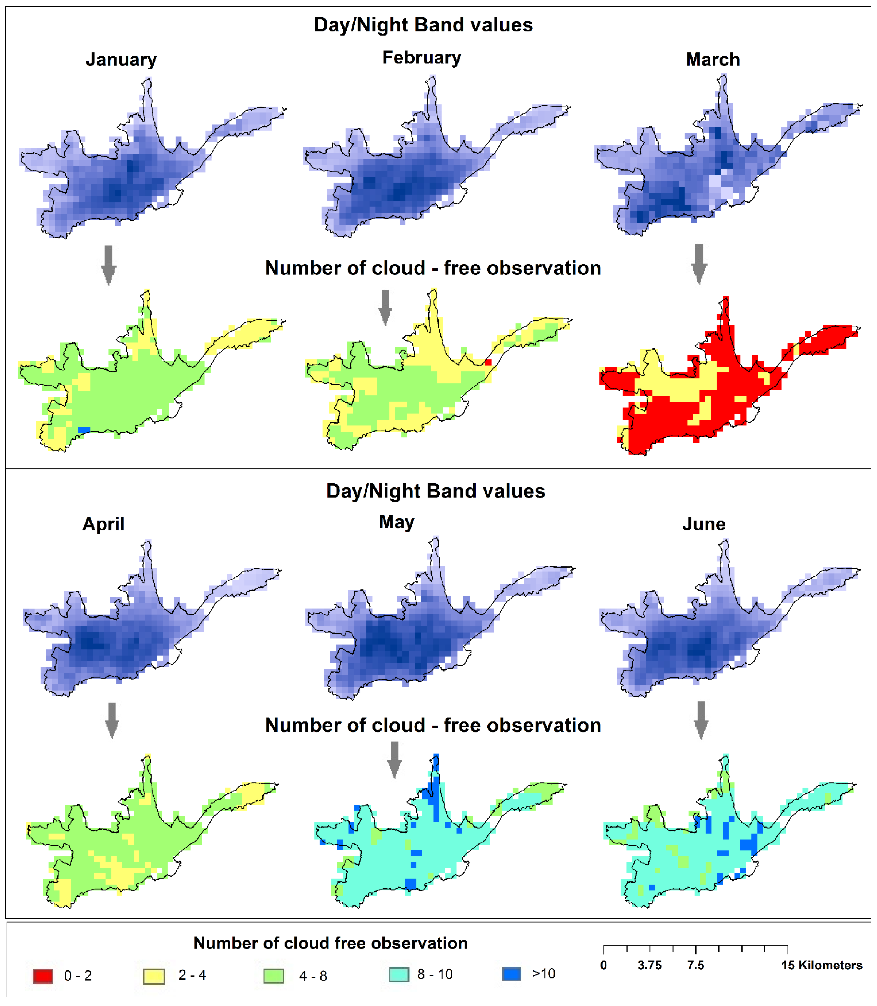
Initial nightlights data selection has a big influence on the model outcome and is particularly important in a sense that VIIRS data is provided by NOAA-NGDC as basic monthly average light intensity composites whereas ISA data comes as a fully-processed product derived from annual DMSP-OLS composites and calibrated with ancillary built-up reference information. The number of cloud-free observations is a crucial factor for producing average composites as excessive cloud cover can obscure light-emitting sources on the ground. In monthly products fewer observations are potentially available to compute composite grids as compared to yearly products and average values can therefore more easily turn out to be skewed and non-representative in case of extended cloud cover in the respective month. There are obviously other influencing parameters that can impair light identification such as obscuring factors like smoke or fog and misleading reflections from snow cover, lightning or the aurora. However, cloud cover is clearly considered the most relevant parameter in the context of the compositing process, particularly in equatorial regions such as the study area of Ecuador. For our study we evaluated the 6 most recent available readily-processed monthly composites (at the time of writing) covering January–June 2015 (other monthly composites were only available as preliminary beta versions having lower quality). For the Cuenca City study area the monthly VIIRS composites of May and June 2015 feature the highest average number of cloud-free observations (see Table 4), thus providing best data reliability.
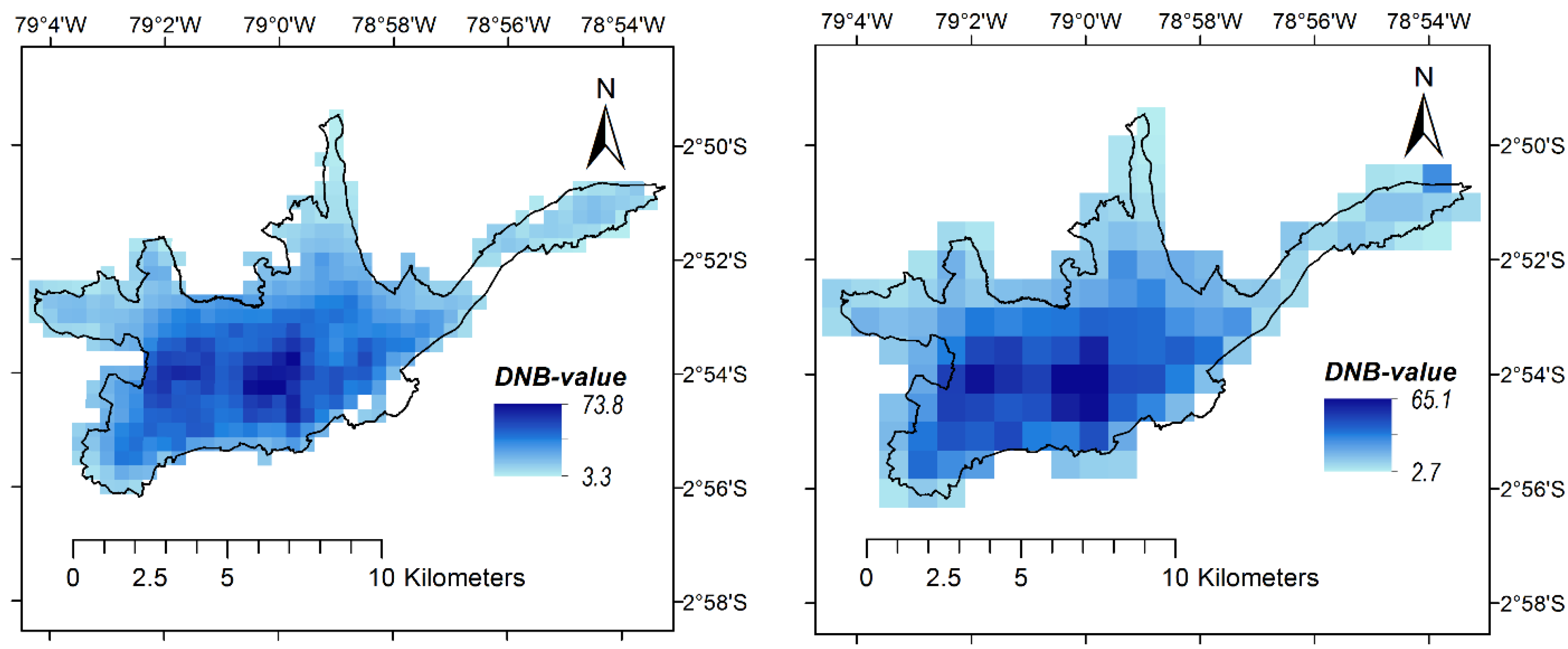
Figure 9 illustrates the light intensity values for the 6 analyzed monthly composites as well as the corresponding number of cloud-free observations at a pixel-by-pixel basis. For the light intensity grids, darker blue tones indicate higher intensity. For the cloud-free observation grids, dark blue would represent the best situation (no cloud cover at any day during the month) whereas green, yellow and red colors indicate decreasing data reliability (due to fewer cloud-free observations).
Table 4. Average number of cloud-free observations in VIIRS 2015 monthly composites for the Cuenca City study area (grey indicating eventually selected monthly composite).
MonthNumber of Cloud-Free ObservationDay/Night Band (DNB) Value
MinMaxAverageMinMax
January295.473.886.9
February264.523.52129.1
March041.980.092.3
April385.373.955.8
May6118.973.555.7
June6118.813.373.8
Theoretically, just a couple of high-quality observations can be sufficient to produce an appropriate composite product. While the monthly composites of May and June have the highest number of cloud-free observations, other months’ composites can thus feature very similar light intensity value distributions (as it is the case for example for the April composite). We therefore explicitly refer to data reliability as an indicator as opposed to general data quality.
Figure 9. VIIRS data of the first six months of 2015 for the Cuenca City study area. Grids of average light intensity (top). Grids showing the number of cloud-free observations at the cell level used to produce the average light intensity composites (bottom).
Remotesensing 08 00114 g009
Although the May composite has the highest number of cloud-free observations on average, that value is almost identical to the June composite (see Table 4). In that case, an additional parameter should be identified to justify selection. On the one hand visual inspection of the cell-level distribution of cloud-free observations could give an extra indication on potential data quality. If, for example, more cloud-free observations are found in the city center (where non-residential activity is expected), that could be beneficial given the context of the presented study. Another parameter could be the detected light intensity range, with detection of higher intensities (i.e., likely non-obscured) being potentially favorable. Following the latter criterion, higher intensity levels are identified in the June composite as compared to the May data set (see Table 4). Other secondary selection criteria could take into account influencing parameters that impair light identification (as mentioned above). Data on those parameters is usually not publicly available though. As intra-urban cloud-free observations at cell-level are similarly distributed for the May and June composites, the higher detected light intensity range was eventually the determining factor in selecting the June data set for the test study.
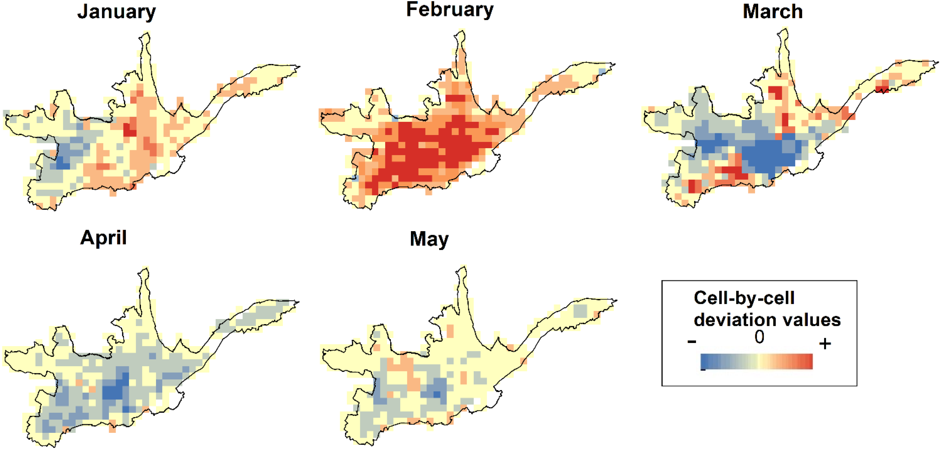
To further highlight the differences in spatial patterns between the 6 available monthly composites, cell-by-cell light intensity deviations of every grid to the eventually selected June composite are computed as illustrated in Figure 10. In line with the observations described above, the May composite matches the June dataset most closely also in that regard. Besides, the overall patterns of those cell-by-cell deviations align adequately with the corresponding grids showing the number of cloud-free observations (see Figure 9). The February and March composites, for example, show the largest deviations to the June grid on a cell-by-cell basis, thus assumingly confirming the poorer reliability of those grids when referring to the low number of cloud-free observations. Specifically the March grid can be considered unusable, while there may be additional reasons for the extreme light intensities observed during the month of February (e.g., night parades and other associated carnival celebration activities in the middle of the month).
Figure 10. Cell-by-cell deviations to the selected June grid.
Remotesensing 08 00114 g010
Table 5 illustrates a set of tested VIIRS threshold values using the May data as alternative in order to demonstrate potential model output variation in case a different monthly composite was selected. When applying the 53rd percentile threshold (highlighted in green in Table 5) that delivered the best match to the cadastral data in the June composite, a 65:35 building use distribution split was obtained for the May composite, thus significantly overestimating the non-residential share. In the May data the 64th percentile is identified as fitting threshold (highlighted in grey in Table 5) best approximating the aggregated cadastral grid.
Table 5. VIIRS distribution thresholds (original 15 arc-sec grid) and corresponding building use distribution ratios using the monthly composite for May ratios (grey indicating selected best-matching threshold, green indicating previously identified June threshold for comparison).
IDVIIRS DistributionBuilt-up Area Distribution
MinThresholdMaxPercentileResidential UseMixed Use
13.516.055.624%32.00%68.00%
23.529.555.650%62.00%37.00%
33.531.155.653%65.00%35.00%
63.537.055.664%75.00%25.00%
93.550.655.690%96.00%4.00%

5.2. Comparative Analysis of ISA- and VIIRS-Based Results of the Binary Land Use Classification

The second aspect to be discussed is a comparison of the model output when using ISA and VIIRS-DNB data respectively. This is relevant in several aspects, most specifically (1) in terms of evaluating feasibility of continued applicability of the presented approach with the DMSP program fading out as well as (2) to assess the impact and examine expected multisided improvements due to VIIRS’ improved spatial and radiometric resolution as compared to OLS.
To factor out potential influences caused by the higher spatial resolution we first compare the findings of the ISA-based analysis to those using a correspondingly aggregated 30 arc-sec VIIRS grid. Results prove to be similar in fact, with a 55th percentile threshold identified as best fit to distinguish residential and mixed occupancy areas in the VIIRS data as compared to the 50% threshold in the ISA data. In case of applying the same 50% threshold to the aggregated VIIRS composite, the obtained occupancy distribution in the correspondingly aggregated cadastral data would show a 70:30 residential-mixed split as compared to the targeted 75:25 ratio. When evaluating the degree of spatial overlap as a measure of model output accuracy, applying the respectively identified best-fitting thresholds to both data sets results in a slightly better capturing of non-residential built-up area in the binary mixed use mask that is derived from the ISA data (83%) as compared to the aggregated VIIRS data based mask (79%). If again the 50% threshold was applied to the VIIRS composite instead of the identified 55th percentile threshold, approximately 84% of the non-residential built-up area would be captured. While thereby a marginally better result is achieved in terms of capturing non-residential built-up area, the residential-mixed distribution ratio would be skewed and mixed use areas would actually be overrepresented spatially.
Applying the VIIRS data in its original spatial resolution (15 arc-sec), the best-fitting threshold value to approximate the targeted 75:25 residential-mixed distribution pattern is identified at the 53rd percentile. This is slightly below the threshold value identified for the aggregated VIIRS composite (55th percentile). 76% of the total non-residential building stock of Cuenca City (3.27 of 4.3 km2) is captured within the derived mixed use mask. That value is below both the 79% value when using the aggregated VIIRS data and the 83% value when using the ISA data. In case of applying the initial 50% threshold for the binary classification, 79% of the non-residential building stock would be captured at a 71:29 occupancy type ratio distribution.
Checking those numbers it therefore appears that using ISA data renders a better model performance than using VIIRS data both in original and aggregated form, inasmuch as more non-residential built-up area is detected in the binary masks that were derived using optimized thresholding to match residential-mixed occupancy distribution ratios. However, while a higher percentage of the non-residential built-up area is captured, ISA-derived mixed use areas are slightly more scattered. Taking VIIRS as input data source clusters the detection more in a sense that the average cell-level non-residential built-up density is higher in those binary occupancy type mask derivatives. Using the original-resolution composite, 76% of the total non-residential building stock (3.27 km2) is captured within 25.75 km2, thus featuring an average non-residential built-up density of 12.7% per km2. When using ISA data, 83% of the total non-residential building stock (3.57 km2) is captured within 32 km2, thus an average density of 11.1% per km2.
With the threshold values and associated parameters are obviously rather similar for the VIIRS- and ISA-based approaches, another interesting evaluative perspective is to derive a corresponding binary mask from the aggregated cadastral data and then check spatial pattern concurrence to the nightlights products. 
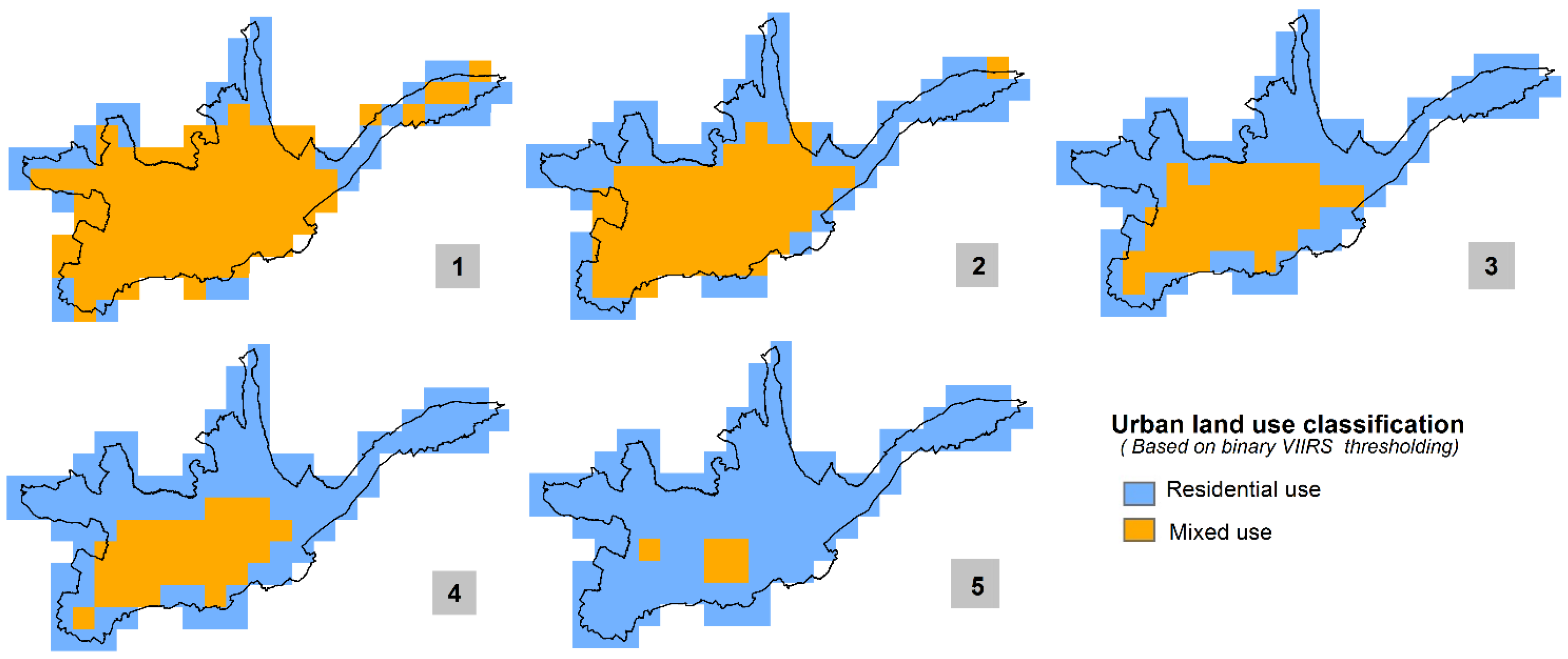
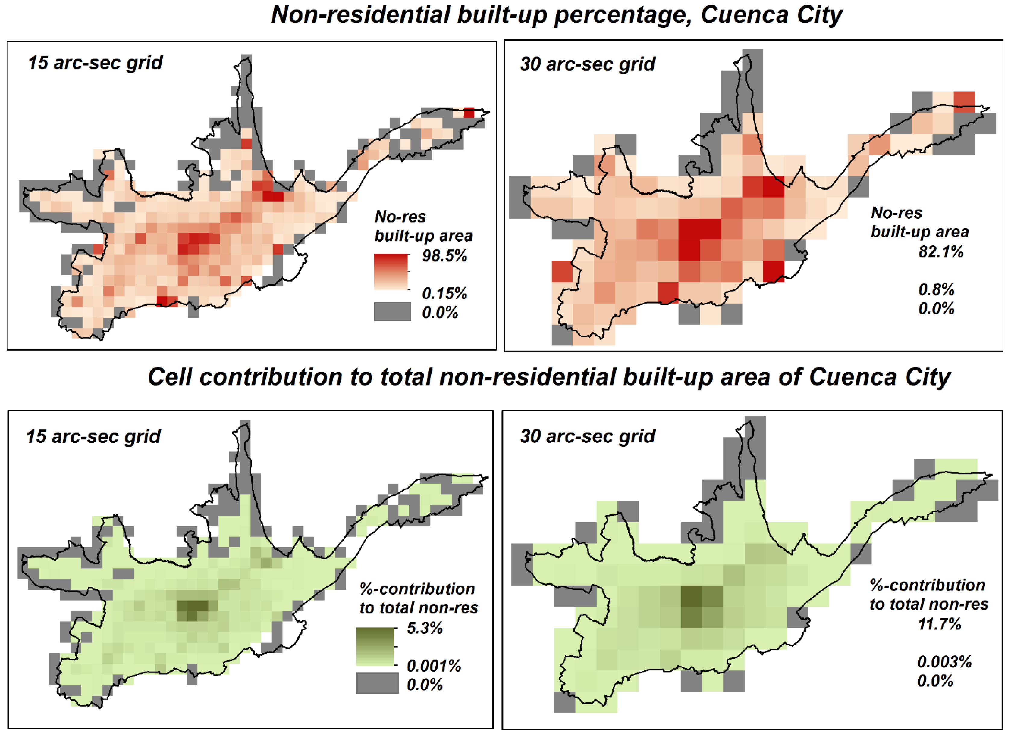
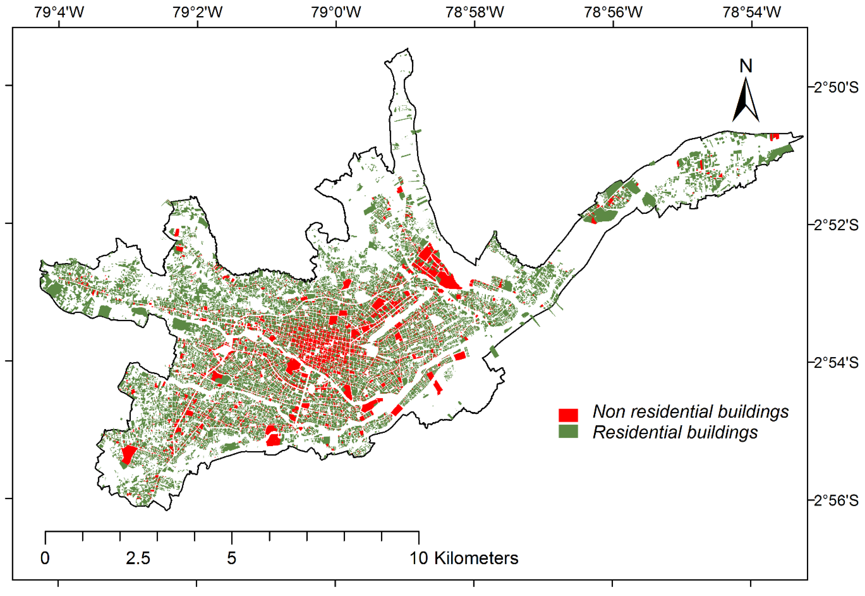
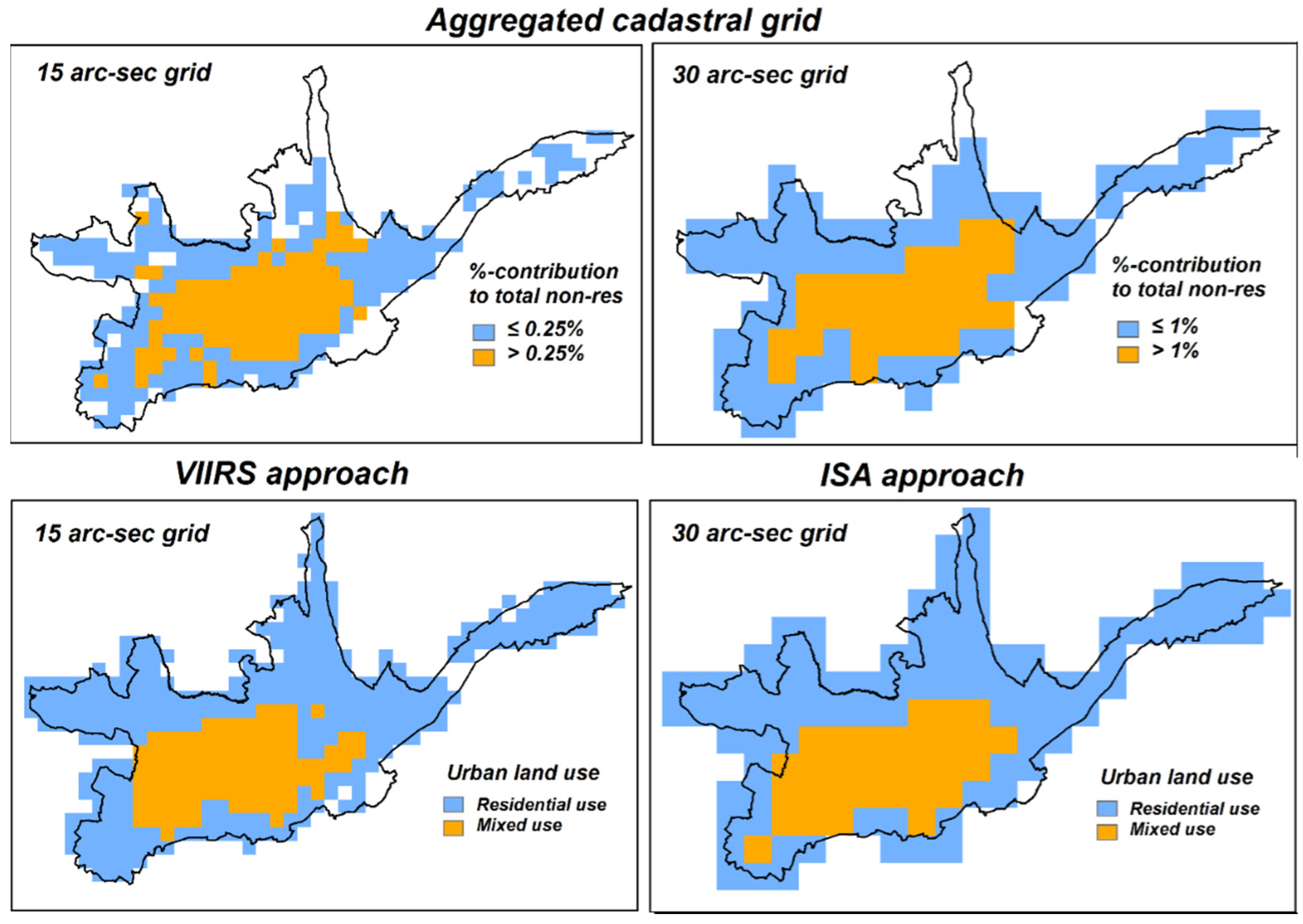
Figure 11 shows the binary classification of the aggregated cadastral data (top), both for the 15 arc-sec (left) and the 30 arc-sec (right) aggregate. The binary mask separates cells that contribute strongly to the total non-residential area from cells that only have a marginal share. This approach is congruent to the nightlights thresholding approach in a sense that it aims at separating high-intensity from low-intensity cells (referring to “non-residential” as observed parameter). The thresholds are determined in a way that, as for the nightlights data thresholding, the 75:25 residential-mixed occupancy type reference ratio split is matched best-possible. For the 15 arc-sec grid the threshold is identified at 0.25% (i.e., cells that have a percent-contribution to the total non-residential area of less or equal than 0.25%), while for the 30 arc-sec grid the derived threshold value is 1%. Interestingly, the difference in fact exactly reflects the scale difference between the two datasets (i.e., factor of 4). The binary 15 arc-sec classification results in a non-residential mask (in dark blue) that captures 88.3% of the total non-residential building area of Cuenca City on an area of 25.5 km2, thus an average density of 14.9% per km2 (compared to the 12.7%/km2 average density in the VIIRS-derived 15 arc-sec binary mask). The 30 arc-sec mask on the other hand captures 86%.
Figure 11. Binary classification of the non-residential cadastral built-up area aggregated to 15 arc-sec (top-left) and 30 arc-sec grids (top-right) based on the percent-contribution to the total non-residential area of Cuenca City. Best-matching binary classifications as derived from 15 arc-sec VIIRS (bottom-left) and 30 arc-sec ISA (bottom-right) data.
Remotesensing 08 00114 g011
For comparative purposes, the bottom two illustrations in Figure 11 show the above-presented best-matching binary masks derived from the 15 arc-sec VIIRS and the 30 arc-sec ISA data. Visually evaluating spatial distribution and extent of the non-residential class in the two maps reveals interesting patterns. The VIIRS-derived mask covers the south-western corner of the corresponding cadaster-based non-residential mask well and misses out on the north-eastern corner whereas it is the other way around with the ISA-derived mask. VIIRS in that context seems not to detect above-average light intensities from the Cuenca City Airport (Aeropuerto Mariscal La Mar), whereas it is a major contributing factor in the ISA data. The latter could be explained with the inherent data configuration of ISA, which per se is more correlated with built-up area rather than pure light intensity.

5.3. Evaluating Model Sensitivity via Application of Different Spatial Urban Delineation

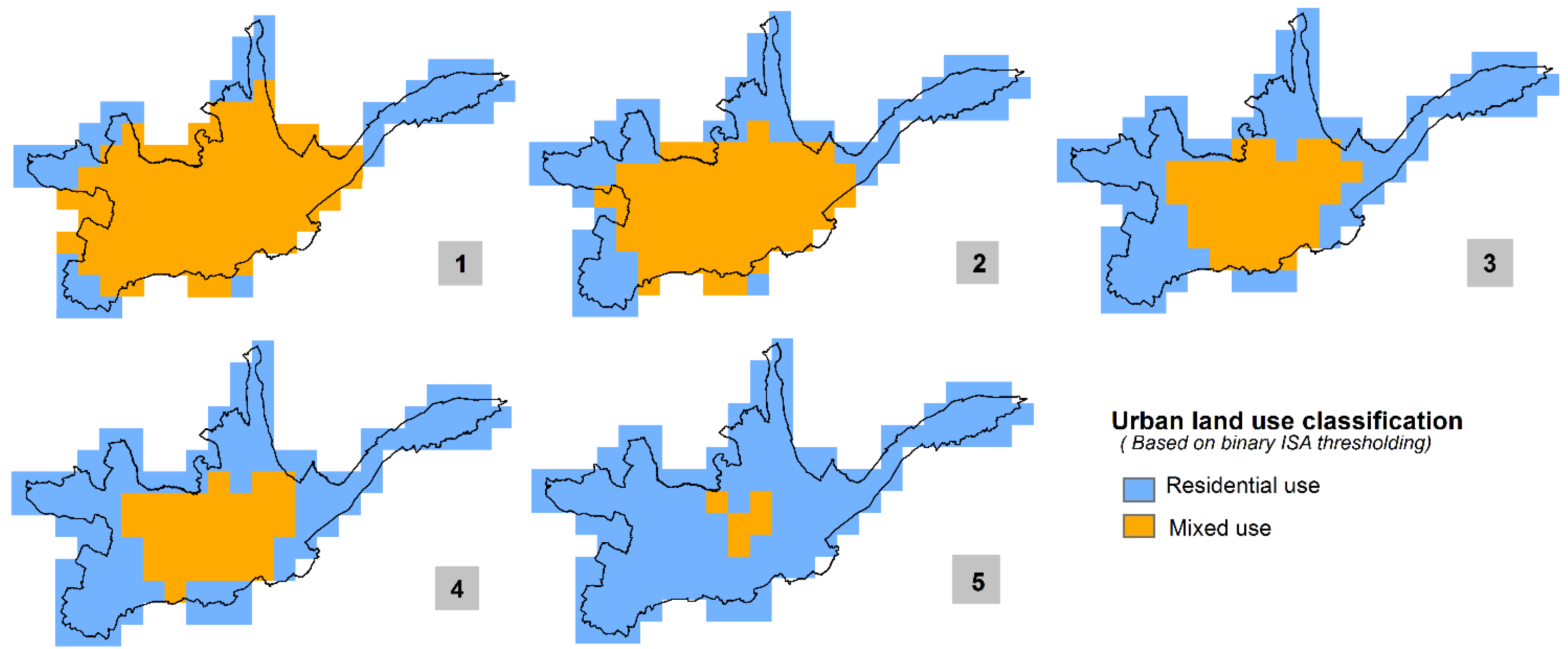
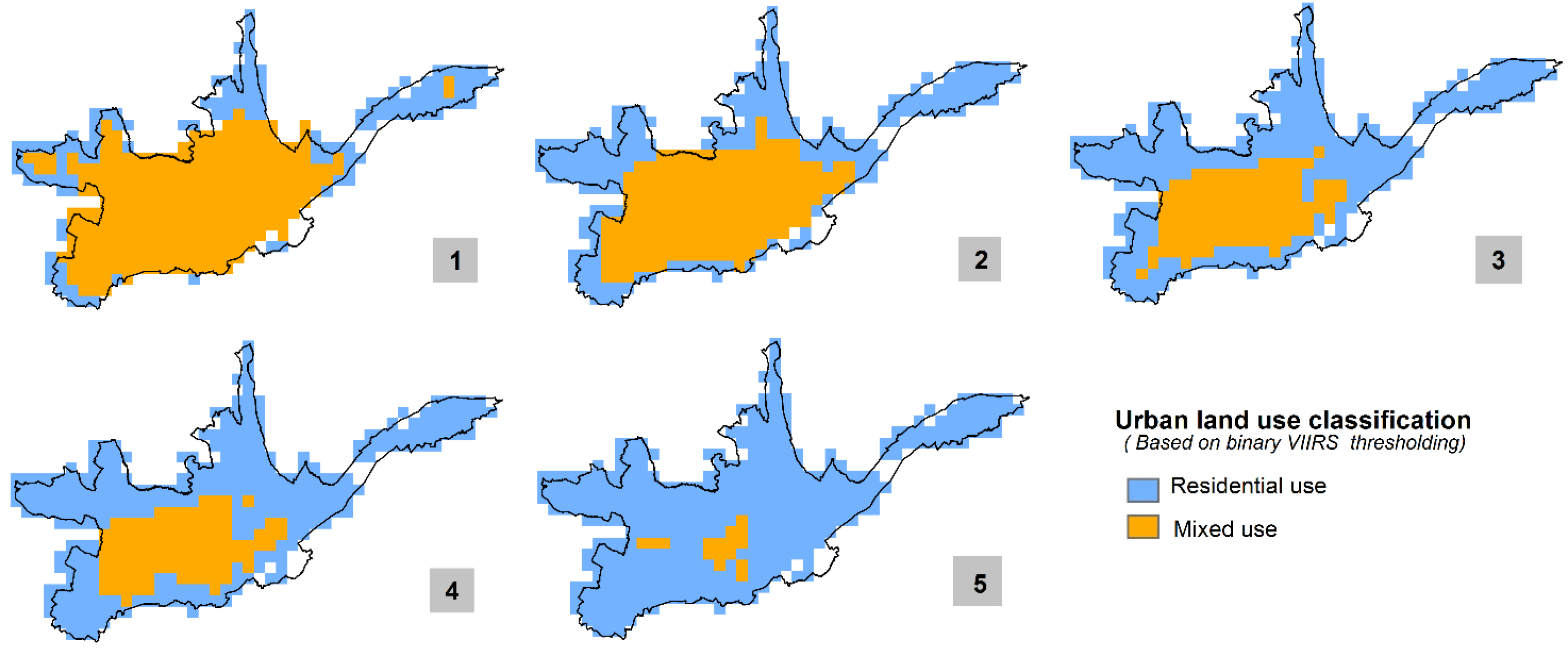
For further evaluation of the model sensitivity we re-run the implemented approach with a geospatially shrunk urban mask. While in the above-outlined implementations all the ISA and VIIRS grid cells were considered that fall within a pre-defined urban area of Cuenca City, now a more central part of the urban agglomeration is selected. Two tests are carried out in that context. For the first one, we keep the same built-up area occupancy type distributions (75% residential vs. 25% mixed use for VRIIS original resolution and 74% residential vs. 26% mixed use for the aggregated grid). In the second test, we keep the same threshold values identified above as the best match, respectively, for each dataset (50th percentile for the ISA data and 53rd percentile for the VIIRS data).
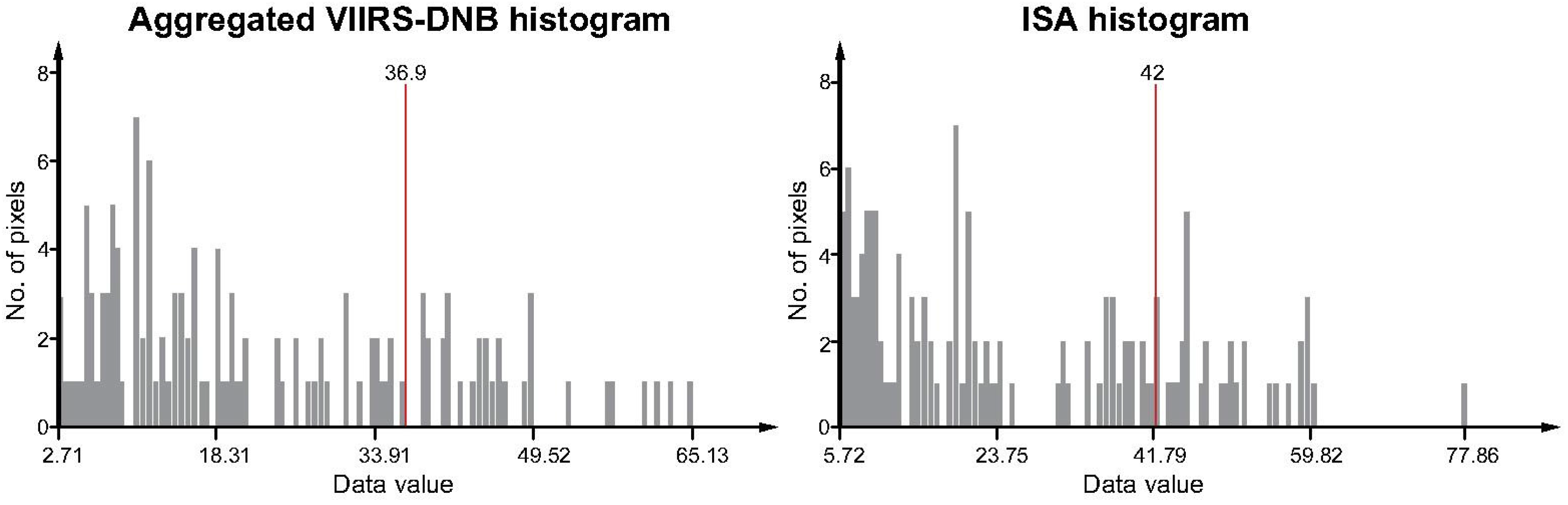
For the first test, the derived best-matching thresholds are now higher for both datasets. For the ISA data the 55th percentile and for the VIIRS-original and aggregated grids the 63rd and 65th percentile are identified respectively. This was expected as predominantly residential areas in the periphery of the city are now not included in the newly-defined urban mask and those cells (featuring lower ISA and light intensity values) are thus missing in the histograms. The threshold increment is higher for the VIIRS data application (roughly 10%–12%-increase) as compared to the ISA data application (5%-increase). This aspect can be associated with different sensitivity of the identified VIIRS and ISA thresholds due to varying histogram distributions (see Figure 12). Given the purpose of the presented modeling, a more even histogram distribution could imply less sensitivity in the threshold determination.
Figure 12. VIIRS-DNB (aggregated) and ISA histograms for the Cuenca city case study.
Remotesensing 08 00114 g012
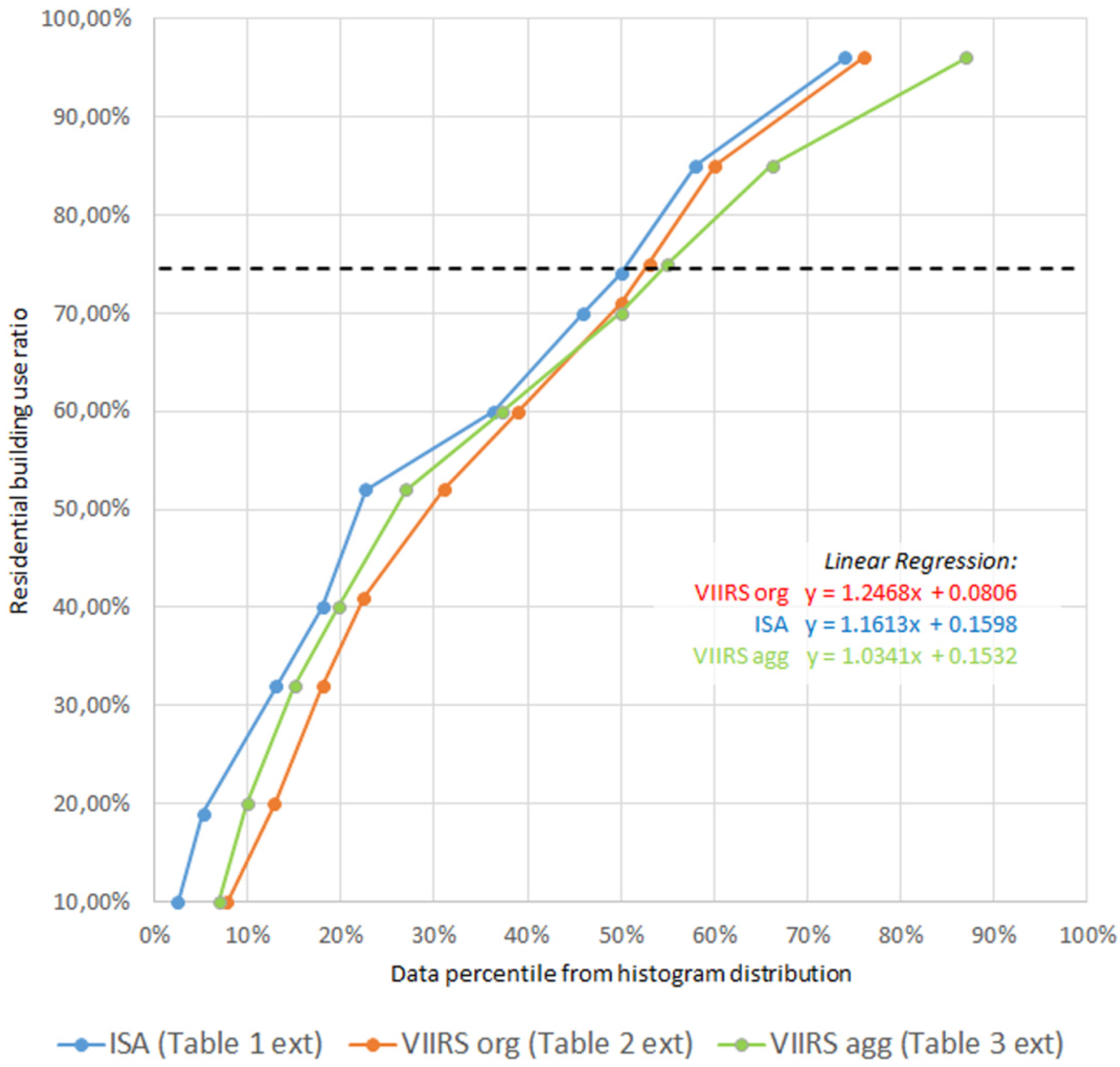
In fact, using the ISA composite, it only takes an increment of 24% (raising the threshold from 50% to 74%) to change the building occupancy type distribution ratio from 74:26 to 96:4. Regarding the aggregated DNB-VIIRS it would require a 35% increment (raising the threshold from 55% to 90%) to achieve the same theoretic change of the built-up area distribution. Small threshold shifts therefore have a bigger impact when using ISA as compared to VIIRS. To illustrate and emphasize this statistically, we use a sample of 10 value pairs each for ISA, original-resolution VIIRS, and aggregated VIIRS as compared to the cadastral building use distribution, and run a linear regression (see Figure 13). Considering all the value pairs, in fact the original-resolution VIIRS data shows the steepest slope in the regression (1.2468) whereas the aggregated VIIRS data indeed show the flattest slope (1.0341) with ISA in between (1.1613). The aggregated VIIRS would thus be the least sensitive to threshold shifting in a sense that the building use distribution ratios would accordingly deviate less from the target value (see dashed line in Figure 13). While steepest when considering all value pairs, the slope of the original VIIRS graph matches ISA almost identically around the relevant target value (dashed line). Threshold shifts in the nightlights products would therefore have a similar impact on the resulting building use distribution ratios.
Figure 13. Plot of residential building use ratio vs. data percentile from histogram distribution for ISA (extended data sample of Table 1), original-resolution VIIRS (extended data sample of Table 2), and aggregated VIIRS (extended data sample of Table 3). The dashed line shows the residential building use ratio for Cuenca City (75%) as derived from cadastral data. Regression equations are colored according to the respective graphs.
Remotesensing 08 00114 g013
In the second test using the best-matching thresholds identified with the initial urban mask (50th percentile for ISA and 53rd and 55th percentile respectively for VIIRS) the newly obtained built-up area occupancy type distribution for the ISA data now corresponds to a 50% residential and 50% mixed use share while for the VIIRS data the distribution now shows a pattern of 56% residential and 44% mixed use considering the original resolution and a 48:52 ratio taking in account the aggregated 30 arc-sec grid. These newly derived built-up area occupancy type distribution patterns are similar for both data sources (ISA and VIIRS) and clearly overestimate the share of mixed use area. This, again, was expected in the same way than the first test result inasmuch as in the selected central part of the urban area there are a decreased number of residential buildings as compared to the sub-urban periphery.
Both tests are correlated in a sense that they give indication on higher light intensity values being clustered in central core urban areas of Cuenca City whereas sub-urban areas feature dimmer lights (and consequently also lower ISA values) on average as a result of higher residential densities. This exercise basically highlights the importance of correct spatial pre-identification of the urban area for subsequent intra-urban analysis. If the urban mask is spatially over- or under-defined, the appropriate nightlights threshold values would de- or increase respectively.

6. Conclusions and Outlook

The presented result of the ISA data application is very interesting as it in fact backs up the prior non-evaluated assumption implemented in the Central American CDRP model to use ISA median values as a threshold for the binary land use classification of residential and mixed use areas. At the continental scale, without ground reference data as are available for the presented Cuenca City test case study, the use of the median value seemed most appropriate as it introduces the least possible subjectivity and merely separates a certain data set in high and low according to its histogram without additionally induced statistical skew.
With that initially assumed median value (50%) threshold for the binary ISA classification confirmed through comparative in situ data analysis for an accurately defined urban agglomeration, the presented case study is considered very beneficial for the overall implementation process of the CDRP initiative. Also, the second re-run of the model with a geospatially shrunken, more central urban mask that showcased the correspondingly expected threshold upward shifts provides another back-up for the model validity as well as underlining the importance of accurate urban delineation in the first place.
It has to be noted that with the presented Cuenca City test case, those findings have to date just been evaluated for that one particular city and caution is advised when it comes to directly transferring those conclusions to other cities. With the CDRP exposure and subsequent risk and loss models already implemented for all of Central America, further test studies can be carried out to increase the sample size of the model evaluation and also test the approach in different regional settings. Cuenca City is considered a rather typical Latin American city with regular patterns of clustered land use within the urban agglomeration. Though, in Central America, basically no major deviations are expected with regard to model applicability, it will be interesting to see testing results when extending to the Caribbean and across as well as to cities of much larger spatial urban extent. Analysis of areas further from the equator may furthermore be influenced by varying seasonal day duration as well as different cloud cover patterns, two parameters which directly affect the nighttime lights compositing.
Testing VIIRS-DNB data as alternative to the DMSP-OLS-based ISA data is considered a crucial step towards a continued applicability of the model. With the DMSP program fading out, VIIRS-DNB is considered the natural successor to the OLS-based nightlights products. With certain visual improvements expected due to VIIRS’s higher spatial and radiometric resolution as compared to OLS, it is still highly valuable to get a clear idea about how these improvements eventually transfer to the binary land use classification output. One specific finding in that context refers to the stronger clustering and thus higher non-residential built-up density in VIIRS-derived binary classification as compared to the ISA-based approach. A major and often-stated benefit of VIIRS with regard to intra-urban pattern analysis is the much-improved radiometric resolution which eliminates the restricting light intensity saturation issues in urban centers in OLS data [21]. For the purpose of the presented study, however, this is not of major relevance as the OLS-derived ISA data refer to a specific radiance-calibrated nightlights product where such saturation issues have already been addressed [32]. Only two ISA datasets are publicly available, however, for the years 2000 and 2010, thus limiting potential direct applicability of the proposed approach in continuous time series analyses. Anyway, even using the annually produced and publicly available OLS stable lights-product would likely not result in a major deterioration of the binary classification as the high intensity values would still be correctly identified irrespective of their relative lower displacement in the histogram due to the saturation issue.
For future studies as well as potential longer-term time series analyses, the finding is very positive in indicating that the DMSP-OLS-based ISA data and the more recent VIIRS data seem to be applicable in very similar fashion as input data sources for the residential-mixed identification model. Two main differences found using VIIRS data concern the varying threshold sensitivity and the amount of built-up detected per square kilometer of land use. The procedure of binary land use classification using VIIRS is considered more flexible than using ISA, and has the potential to give a finer-scale classification of residential and mixed used in urban areas.

Acknowledgments

The findings, interpretations, and conclusions expressed in this paper are entirely those of the authors. They do not necessarily represent the views of the International Bank for Reconstruction and Development/World Bank and its affiliated organizations, or those of its Executive Directors or the governments they represent. Support from the World Bank’s Probabilistic Risk Assessment Program (CAPRA) and the associated Country Disaster Risk Profiles (CDRP) initiative is acknowledged. An earlier and less comprehensive version of this article showing preliminary results was presented as contribution to the 1st International Electronic Conference on Remote Sensing (ECRS-1). The concepts discussed are grounded within recent work on setting up a global-scale exposure model within the framework of the CDRP initiative, implemented in Central America and the Caribbean. The authors appreciate initial conceptual discussions within the CDRP team, specifically with Rashmin Gunasekera and Oscar Ishizawa, as well as comments from four anonymous reviewers that helped improve the quality of the paper.

Author Contributions

Christoph Aubrecht developed the conceptual framework for the presented top-down method and tested geospatial implementation in various Central American countries in the context of the CDRP project initiative. José Antonio León Torres then implemented the developed approach for the Cuenca City (Ecuador) case study and performed the comparative analysis with the bottom-up cadastral data. Following up on the successful presentation of first results at the ECRS-1 conference, further research was carried out regarding the additional integration of alternative nighttime EO data sources, leading to the multi-sensor approach illustrated in this paper. Christoph Aubrecht developed that idea conceptually and José Antonio León Torres again implemented for the Cuenca City test site. The paper was initiated by Christoph Aubrecht, with major contributions from both authors in all sections.

Conflicts of Interest

The authors declare no conflict of interest.

References

  1. United Nations. World Urbanization Prospects: The 2014 Revision; United Nations: New York, NY, USA, 2014. [Google Scholar]
  2. World Bank. World Development Report 2014: Risk and Opportunity—Managing Risk for Development; World Bank: Washington, DC, USA, 2014. [Google Scholar]
  3. World Bank & International Monetary Fund. Global Monitoring Report 2015/2016: Development Goals in an Era of Demographic Change; World Bank: Washington, DC, USA, 2016. [Google Scholar]
  4. Gunasekera, R.; Ishizawa, O.; Aubrecht, C.; Murray, S.; Blankespoor, B.; Pomonis, A.; Daniell, J. Developing an Adaptive Exposure Model to Support the Generation of Country Disaster Risk Profiles. Earth-Sci. Rev. 2015, 150, 594–608. [Google Scholar] [CrossRef]
  5. Aubrecht, C.; Gunasekera, R.; Ishizawa, O. Urban characterization aspects and associated spatial scale considerations in the context of global-level exposure modeling: Comparative data evaluation. In Proceedings of the Second European Conference on Earthquake Engineering and Seismology (2ECEES), Istanbul, Turkey, 24–29 August 2014.
  6. Jaiswal, K.; Wald, D.; Porter, K. A Global Building Inventory for Earthquake Loss Estimation and Risk Management. Earthq. Spectra 2010, 26, 731–748. [Google Scholar] [CrossRef]
  7. Elvidge, C.D.; Tuttle, B.T.; Sutton, P.C.; Baugh, K.E.; Howard, A.T.; Milesi, C.; Bhaduri, B.; Nemani, R. Global Distribution and Density of Constructed Impervious Surfaces. Sensors 2007, 7, 1962–1979. [Google Scholar] [CrossRef]
  8. Miller, S.D.; Mills, S.P.; Elvidge, C.D.; Lindsey, D.T.; Lee, T.F.; Hawkins, J.D. Suomi satellite brings to light a unique frontier of nighttime environmental sensing capabilities. Proc. Natl. Acad. Sci. USA 2012, 109, 15706–15711. [Google Scholar] [CrossRef] [PubMed]
  9. Aubrecht, C.; León Torres, J.A. Top-down identification of mixed vs. residential use in urban areas: Evaluation of remotely sensed nighttime lights for a case study in Cuenca City, Ecuador. In Proceedings of the 1st International Electronic Conference on Remote Sensing (ECRS-1), 22 June–5 July 2015; 2015; Volume 1, p. d005. [Google Scholar] [CrossRef]
  10. Welch, R. Monitoring urban population and energy utilization patterns from satellite data. Remote Sens. Environ. 1980, 9, 1–9. [Google Scholar] [CrossRef]
  11. Elvidge, C.D.; Baugh, K.E.; Kihn, E.A.; Kroehl, H.W.; Davis, E.R.; Davis, C.W. Relation between satellite observed visible-near infrared emissions, population, economic activity and electric power consumption. Int. J. Remote Sens. 1997, 18, 1373–1379. [Google Scholar] [CrossRef]
  12. Sutton, P.; Roberts, D.; Elvidge, C.; Baugh, K. Census from Heaven: An estimate of the global human population using night-time satellite imagery. Int. J. Remote Sens. 2001, 22, 3061–3076. [Google Scholar] [CrossRef]
  13. Doll, C.N.H.; Muller, J.-P.; Morley, J.G. Mapping regional economic activity from night-time light satellite imagery. Ecol. Econ. 2006, 57, 75–92. [Google Scholar] [CrossRef]
  14. Sutton, P.C.; Cova, T.J.; Elvidge, C.D. Mapping “Exurbia” in the conterminous United States using nighttime satellite imagery. Geocarto Int. 2006, 21, 39–45. [Google Scholar] [CrossRef]
  15. Elvidge, C.; Sutton, P.C.; Tuttle, B.T.; Ghosh, T.; Baugh, K.E. Global urban mapping based on nighttime lights. In Global Mapping of Human Settlement; Gamba, P., Herold, M., Eds.; CRC Press: Boca Raton, FL, USA, 2009; pp. 129–144. [Google Scholar]
  16. Zhou, Y.; Smith, S.J.; Elvidge, C.D.; Zhao, K.; Thomson, A.; Imhoff, M. A cluster-based method to map urban area from DMSP/OLS nightlights. Remote Sens. Environ. 2014, 147, 173–185. [Google Scholar] [CrossRef]
  17. Rich, C.; Longcore, T. Ecological Consequences of Artificial Night Lighting, 1st ed.; Island Press: Washington, DC, USA, 2006. [Google Scholar]
  18. Aubrecht, C.; Elvidge, C.D.; Longcore, T.; Rich, C.; Safran, J.; Strong, A.E.; Eakin, C.M.; Baugh, K.E.; Tuttle, B.T.; Howard, A.T.; et al. A global inventory of coral reef stressors based on satellite observed nighttime lights. Geocarto Int. 2008, 23, 467–479. [Google Scholar] [CrossRef]
  19. Rodrigues, P.; Aubrecht, C.; Gil, A.; Longcore, T.; Elvidge, C. Remote sensing to map influence of light pollution on Cory’s shearwater in São Miguel Island, Azores Archipelago. Eur. J. Wildlife Res. 2012, 58, 147–155. [Google Scholar] [CrossRef]
  20. Elvidge, C.D.; Imhoff, M.L.; Baugh, K.E.; Hobson, V.R.; Nelson, I.; Safran, J.; Dietz, J.B.; Tuttle, B.T. Night-time lights of the world: 1994–1995. ISPRS J. Photogramm. Remote Sens. 2001, 56, 81–99. [Google Scholar] [CrossRef]
  21. Elvidge, C.D.; Baugh, K.E.; Zhizhin, M.; Hsu, F.-C. Why VIIRS data are superior to DMSP for mapping nighttime lights. Proc. Asia-Pac. Adv. Netw. 2013, 35, 62–69. [Google Scholar] [CrossRef]
  22. Levin, N.; Johansen, K.; Hacker, J.M.; Phinn, S. A new source for high spatial resolution night time images—The EROS-B commercial satellite. Remote Sens. Environ. 2014, 149, 1–12. [Google Scholar] [CrossRef]
  23. Elvidge, C.D.; Milesi, C.; Dietz, J.B.; Tuttle, B.T.; Sutton, P.C.; Nemani, R.; Vogelmann, J.E. U.S. constructed area approaches the size of Ohio. EOS Trans. Am. Geophys. Union 2004, 85, 233–240. [Google Scholar] [CrossRef]
  24. Potere, D.; Schneider, A.; Angel, S.; Civco, D. Mapping urban areas on a global scale: Which of the eight maps now available is more accurate? Int. J. Remote Sens. 2009, 30, 6531–6558. [Google Scholar] [CrossRef]
  25. Esch, T.; Taubenböck, H.; Roth, A.; Heldens, W.; Felbier, A.; Thiel, M.; Schmidt, M.; Müller, A.; Dech, S. TanDEM-X mission—New perspectives for the inventory and monitoring of global settlement patterns. J. Appl. Remote Sens. 2012, 6. [Google Scholar] [CrossRef]
  26. Pesaresi, M.; Huadong, G.; Blaes, X.; Ehrlich, D.; Ferri, S.; Gueguen, L.; Halkia, M.; Kauffmann, M.; Kemper, T.; Lu, L.; et al. A global human settlement layer from optical HR/VHR RS data: Concept and first results. IEEE J. Sel. Top. Appl. Earth Observ. Remote Sens. 2013, 6, 2102–2131. [Google Scholar] [CrossRef]
  27. Baugh, K.; Hsu, F.-C.; Elvidge, C.; Zhizhin, M. Night lights compositing using the VIIRS day-night band: Preliminary results. Proc. Asia-Pac. Adv. Netw. 2013, 35, 70–86. [Google Scholar] [CrossRef]
  28. Municipalidad de Cuenca (GAD). Catastro Urbana de la Ciudad de Cuenca; Departamento de Avalúos y Catastros: Cuenca, Ecuador, 2015. [Google Scholar]
  29. Foody, G.M.; Cox, D.P. Sub-pixel land cover composition estimation using a linear mixture model and fuzzy membership functions. Int. J. Remote Sens. 1994, 15, 619–631. [Google Scholar] [CrossRef]
  30. Fisher, P. The pixel: A snare and a delusion. Int. J. Remote Sens. 1997, 18, 679–685. [Google Scholar] [CrossRef]
  31. Aubrecht, C.; Gunasekera, R.; Ishizawa, O.; Pita, G. The flipside of “urban”—A novel model for built-up-adjusted rural-urban pattern identification and population reallocation. In Internal CDRP Working Paper 2015; World Bank: Washington, DC, USA, 2015. [Google Scholar]
  32. Elvidge, C.D.; Baugh, K.E.; Dietz, J.B.; Bland, T.; Sutton, P.C.; Kroehl, H.W. Radiance calibration of DMSP-OLS low-light imaging data of human settlements. Remote Sens. Environ. 1999, 68, 77–88. [Google Scholar] [CrossRef]

