Elevation Change Rates of Glaciers in the Lahaul-Spiti (Western Himalaya, India) during 2000–2012 and 2012–2013

Abstract

Previous studies have shown contrasting glacier elevation and mass changes in the sub-regions of high-mountain Asia. However, the elevation changes on an individual catchment scale can be potentially influenced by supraglacial debris, ponds, lakes and ice cliffs besides regionally driven factors. Here, we present a detailed study on elevation changes of glaciers in the Lahaul-Spiti region derived from TanDEM-X and SRTM C-/X-band DEMs during 2000–2012 and 2012–2013. We observe three elevation change patterns during 2000–2012 among glaciers with different extent of supraglacial debris. The first pattern (<10% debris cover, type-1) indicates maximum thinning rates at the glacier terminus and is observed for glaciers with no or very low debris cover. In the second pattern (>10% debris cover, type-2), maximum thinning is observed up-glacier instead of glacier terminus. This is interpreted as the insulating effect of a thick debris cover. A third pattern, high elevation change rates near the terminus despite high debris cover (>10% debris cover, type-3) is most likely associated with either thinner debris thickness or enhanced melting at supraglacial ponds and lakes as well as ice cliffs. We empirically determined the SRTM C- and X-band penetration differences for debris-covered ice, clean ice/firn/snow and correct for this bias in our elevation change measurements. We show that this penetration bias, if uncorrected, underestimates the region-wide elevation change and geodetic mass balance by 20%. After correction, the region-wide elevation change (1712 km${}^2$) was estimated to be −0.65 ± 0.43 m yr${}^{-1}$ during 2000–2012. Due to the short observation period, elevation change measurements from TanDEM-X for selected glaciers in the period 2012–2013 are subject to large uncertainties. However, similar spatial patterns were observed during 2000–2012 and 2012–2013, but at different magnitudes. This study reveals that the thinning patterns of debris-covered glaciers cannot be generalized and spatially detailed mapping of glacier elevation change is required to better understand the impact of different surface types under changing climatic conditions.

1. Introduction

Hindu Kush-Pamir-Karakoram-Himalaya (HKPKH) is a widely spread mountain range in high-mountain Asia with a glacial extent of ∼60,100 km${}^2$ [1]. A segment is located in the Lahaul-Spiti region of western Himalaya, India. The glaciers in the Lahaul-Spiti receive precipitation throughout the year but majorly during July–September by Indian summer monsoon (ISM) and during January–April by mid-latitude winter westerlies (MLW) [2]. The warming trend of surface air temperature (e.g., 0.46${}^{\circ }$ per decade during 1971–2007) in western Himalaya is higher than the global average [3]. These increasing air temperatures have substantial implications on glacier mass balance as they foster ablation [4]. Therefore, glacier mass balance has been considered as the most appropriate variable in order to assess glacier status and its response to climate change.

Previous studies have revealed that the pattern of glacier elevation (and mass) changes in the HKPKH region is heterogeneous. Using ICESat (Ice, Cloud and land Elevation Satellite) laser altimetry, Kääb et al. [1] showed almost balanced mass budgets for the Karakoram region during 2003–2009, while for surrounding regions, including the Lahaul-Spiti region, considerable surface lowering was observed. They also reported comparable lowering rates for debris-covered and debris-free glaciated areas in high-mountain Asia based on the region-wide average assessment. However, other authors noted much more spatially heterogeneous surface lowering rates possibly due to glacier orientation [5], supraglacial debris cover distribution [6], supraglacial water bodies and ice cliffs [7]. Usually the ice which is fully exposed to solar radiation melts with higher rates. A thin debris cover might absorb more radiation and transfer the heat to the ice beneath leading to even higher rates of melt [8]. Similarly, supraglacial water bodies and ice cliffs also enhance the melting of ice [9,10,11]. Contrary to these triggering effects, a thick debris cover protects the underlying ice and reduces melt [6,8,12].

The Lahaul Spiti region comprises glaciers with different settings—sparse or extensive debris coverages, supraglacial water bodies and ice cliffs. For instance, Bara Shigri Glacier in the Lahaul-Spiti region is highly debris-covered (∼18%) to a certain altitude, which includes ∼60–70 supraglacial lakes and ice cliffs [13]. Gardelle et al. [14] showed glacier mass changes of −0.45 ± 0.13 m w.e. yr${}^{-1}$ (1999–2011) based on a comparison of SRTM (Shuttle Radar Topography Mission) and SPOT5 (Système pour l’Observation de la Terre) DEMs for the entire Lahaul Spiti region. However, this study was limited since it only covered 46% of the glacierized area (2110 km${}^2$) due to clouds. Moreover, the authors assumed that the difference between C- and X-band radar penetration of SRTM during winter conditions was similar to the difference between the surface and the C-band scattering phase center. This assumption has been proved incorrect by subsequent studies (e.g., [15], 2016 for the French Alps), but also by analyses for other regions revealing up to 10 m X-band radar penetration into dry snow [16].

The outline above demonstrates that detailed studies on the influence of different supraglacial features (debris, ponds, lakes and ice cliffs) on glacier elevation changes as well as overall improved estimates are required. Hence, the aims of this study are:

• to provide spatially detailed elevation change estimates of glaciers in the Lahaul Spiti region based on X-/C-band synthetic aperture radar interferometry;
• to assess the potential of the TanDEM-X (TerraSAR-X add-on for DEM Measurements) mission (X-band) to measure glacier elevation changes in one year time scale;
• to estimate the impact of X-/C-band penetration into glaciers and its implications for region-wide surface elevation change estimates;
• to investigate several glacier properties (e.g., supraglacial debris coverage, supraglacial lakes, ponds, ice cliffs etc.) to explain glacier elevation change.

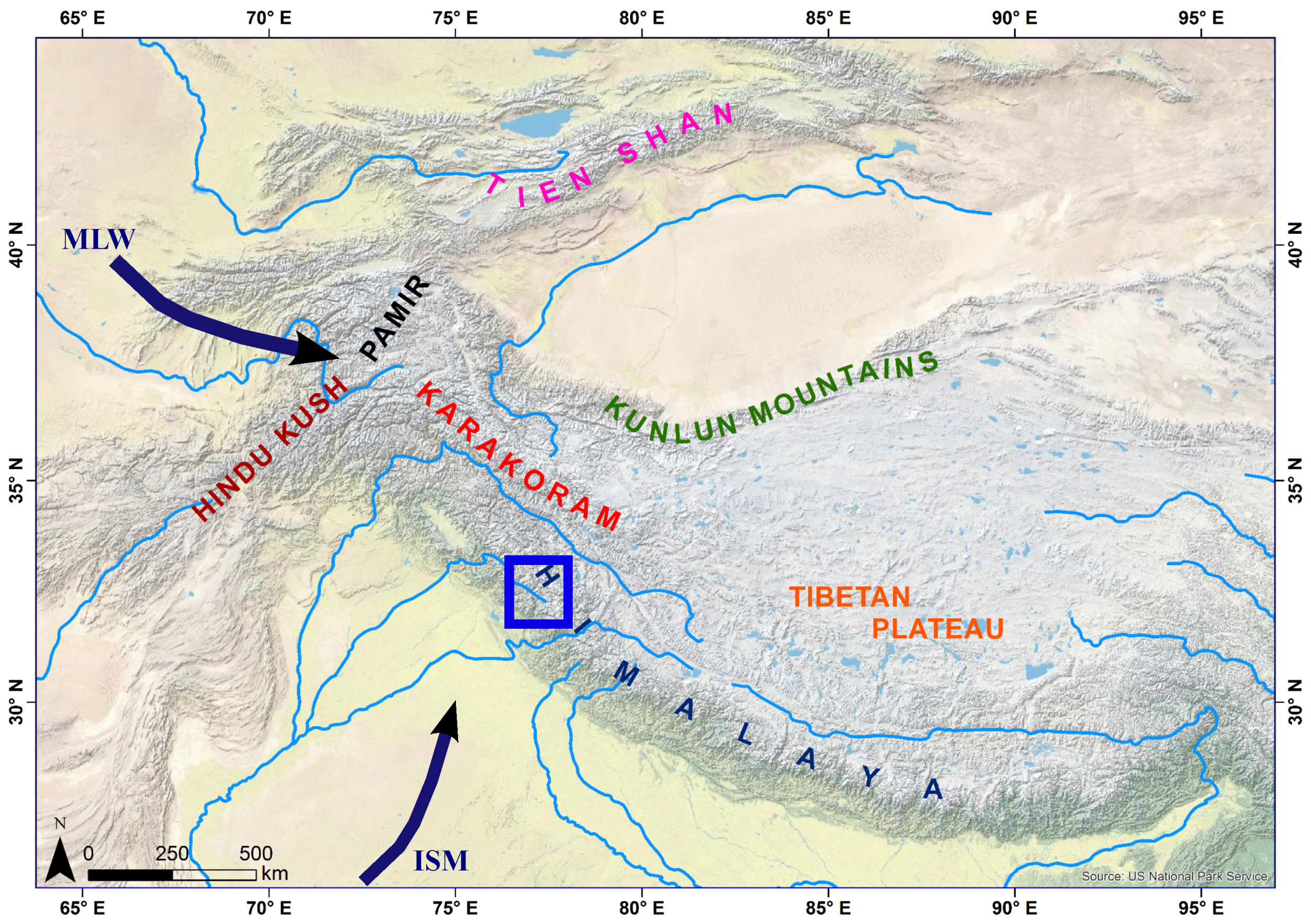
2. Study Area

The study region (Lahaul-Spiti) is located in the western Himalaya, India (Figure 1). The region comprises more than 1400 glaciers (∼2110 km${}^2$) [5] which feed many sub-basins of the Indus river providing freshwater resource for downstream infrastructural necessities. Chhota Shigri (32.2${}^{\circ }$N, 77.5${}^{\circ }$E) is a benchmark glacier of the region [17] where comprehensive observations have been carried out since 2002 [5,17,18]. Meteorological observations (1969–2012) at the Bhuntar Observatory at 1092 m a.s.l. (31.5${}^{\circ }$N, 77.9${}^{\circ }$E) suggest that Chhota Shigri Glacier lies at a transit zone of the ISM and the MLW and is almost similarly influenced by both wind systems [19]. However, the MLW seem to dominate (∼71% of the annual precipitation) during 2012–2013 as measurements at the glacier base camp at 3850 m a.s.l. suggest [18].

Overall, 22% of the observed glaciated area in the region is debris-covered. Many glaciers have extensive debris coverage (>10%). The debris material varies from fine-grained silt to large boulders ranging from a few milimeters to several meters in thickness [5]. In the debris-covered parts of many glaciers, supraglacial lakes, ponds and ice cliffs are often present. The majority of the glaciers are land-terminating, but the terminus of Samudra Tapu Glacier (32.5${}^{\circ }$N, 77.5${}^{\circ }$E) and $G077241E32946N$ (32.94${}^{\circ }$N, 77.24${}^{\circ }$E) terminate to lakes.

3. Data

The Shuttle Radar Topography Mission (SRTM) acquired interferometric synthentic aperture radar (InSAR) data in X- and C-band radar frequencies between 11 and 22 of February 2000. The SRTM X-band DEM does not have a global coverage as it was acquired with a ScanSAR mode and without post-processing [20]. Therefore, the void filled SRTM C-band DEM of 1 arcsec grid spacing, originally referenced to EGM96 geoid, was used as reference DEM in our TanDEM-X processing chain to measure elevation change. The SRTM X-band DEM with 1 arcsec, referenced to WGS84 ellipsoid, was used to determine the C- and X-band penetration difference bias. TanDEM-X is a German bistatic mission operated by the German Aerospace Center (DLR) and EADS ASTRIUM consisting of two nearly identical satellites which simultaneously acquire single-pass InSAR data [21]. The DLR provides these two acquired images as coregistered single look complex images (CoSSC) in HH polarization. The exact date, time and other interferometric parameters of the TanDEM-X datasets of this study are listed in

Table 1. The specifications of TanDEM-X images used in the study. These specifications include year, date and time of the TanDEM-X data acquisitions, orbital pass, effective baseline (B${}_{eff}$), height of ambiguity (HoA), incidence angle. The differential phase of TanDEM-X data was either unwrapped with Minimum Cost Flow (MCF) and Branch Cut (BC) algorithm (Section 4.1.1).

S.No.	Date (Day Month Year)	Time (HH:MM:SS)	Orbit	B${}_{\mathit{e}\mathit{f}\mathit{f}}$ (m)	HoA (m)	Incidence Angle (${}^{\circ }$)	Phase Unwrapping
1	29 January 2012	12:45:46	Ascending	82.31	−75.73	38.52	BC
2	29 January 2012	12:45:53	Ascending	82.53	−75.74	38.54	BC
3	9 February 2012	12:45:39	Ascending	83.98	−68.76	36.29	MCF
4	9 February 2012	12:45:46	Ascending	84.21	−68.30	36.22	BC
5	9 February 2012	12:45:53	Ascending	84.37	−68.26	36.28	BC
6	20 February 2012	12:45:52	Ascending	88.67	59.14	33.69	MCF
7	26 January 2013	12:45:52	Ascending	130.09	45.10	37.09	MCF
8	26 January 2013	12:45:58	Ascending	130.24	45.04	37.08	MCF

. A cloud free Landsat-7 Enhanced Thematic Mapper (ETM) scene of 15 October 2000 was selected to map the glacier surface type. Glacier outlines were taken from the recently published Randolph Glacier Inventory (RGI 5.0) [22,23].

4. Methods

4.1. Elevation Change

We measured surface elevation change in two time periods (2000–2012 and 2012–2013). In a first step, we applied interferometric processing (InSAR) over all bistatic TanDEM-X pairs. This provided the elevation change in regard to the SRTM-C DEM and absolute elevation (TanDEM-X DEM) for every processed scene. Secondly, the adjacent scenes were mosaicked to quantify elevation change and to generate a TanDEM-X DEM for the entire study area. In the last step, we measured the penetration difference between SRTM C- and X-band over different surface types (off-glacier, debris-covered ice, clean ice/firn/snow) and corrected for this bias for the entire glaciated area.

4.1.1. Interferometric Processing

Synthetic aperture radar interferometry (InSAR) is a sequential procedure to generate DEMs and estimate terrain deformation (e.g., elevation changes). In our processing scheme, we used a reference DEM and a complex SAR image pair. Therefore, we deployed the SRTM-C DEM as a reference DEM jointly with the bistatic TanDEM-X pair for InSAR processing [24]. We first simulated the topographic phase from the SRTM-C DEM using TanDEM-X interferometric parameters (baseline, slant range distance, look angle etc.). The simulated topographic phase was then subtracted from the complex interferometric phase of the TanDEM-X pair in order to form a double difference interferogram. We removed the phase noise from the double difference interferogram using a Goldstein filter with a filtering coefficient (${\alpha }_{filter}$) of 0.35 (${\alpha }_{filter}$ ∈ [0,1]). The areas degraded due to layover, foreshortening, shadow and water bodies (coherence < 0.3) were masked out before unwrapping the double difference interferogram using branch cut (BC) [25] and minimum cost flow (MCF) [26] algorithms. We opted for the unwrapped product from either the BC or MCF depending on the least phase unwrapping errors (phase jumps, phase residuals etc.). The starting point of the phase unwrapping was carefully chosen on stable ground keeping the differential phase of this point at 0.0 radians, as it was assumed to be unchanging between SRTM and TanDEM-X data acquisitions. The unwrapped differential phase was then converted into differential heights, also referred to elevation change with reference to the SRTM-C DEM. Subsequently, these differential heights were added back to the topographic heights from SRTM-C DEM to generate a TanDEM-X DEM. The resulting TanDEM-X DEM and differential heights were geocoded with the SRTM-C DEM in order to keep planimetric consistency. Finally, the resulting products were corrected for tropospheric path delays following the approach in [27].

4.1.2. Mosaicking

We mosaicked the adjacent TanDEM-X scenes (Table 1) for maximum coverage of the region in a two step approach. In the first step, all TanDEM-X scenes were adjusted to the SRTM-C DEM with the median deviation, determined over stable terrain (off-glacier). In the second step, we double checked the vertical alignment of the adjacent scenes using a linear regression test. For this, we chose randomly distributed points over stable and non-glaciated ground in the overlapping area of the scenes. In an ideal scenario, the linear regression test (p = aq + b) should give a = 1 and b = 0 on stable terrain. Here, p and q depict the elevations from adjacent DEMs. In all cases, we found a = 1 and b < 0.2 m (0.02 m yr${}^{-1}$) with R${}^2$ value of 0.99 which signifies high degree of vertical alignment of our products. Finally the resulting products were corrected for this remaining offset (b) before mosaicking.

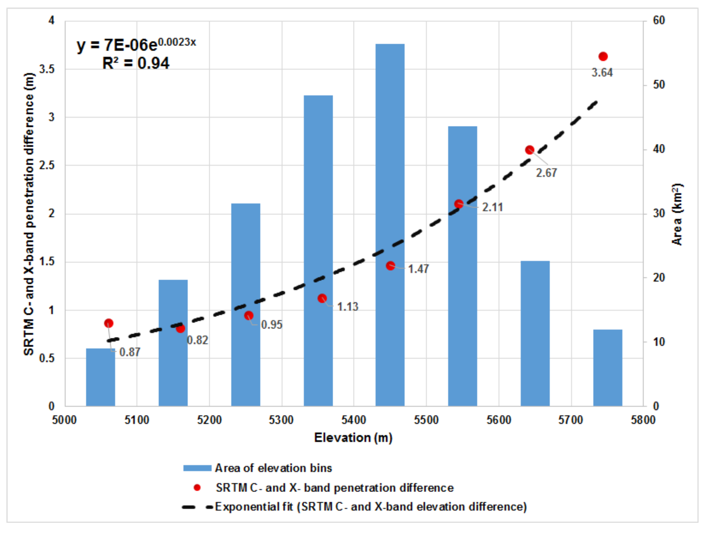
4.1.3. SRTM C- and X-Band Penetration Difference

The direct analysis of TanDEM-X (X-band) and SRTM-C (C-band) DEM differencing for elevation change measurements is restricted due to the potential bias of variable X- and C-band radar signal penetration into the glacier surface [28]. Therefore, we compared the elevation difference from SRTM X-band and C-band DEMs over different surfaces (off-glacier, debris-covered ice, clean ice/firn/snow) in our study area. The vertical datum of the SRTM X-band DEM was converted into the Earth Gravity Model 1996 geoid (EGM96), similar as of SRTM C-band DEM, before this comparison. We vertically adjusted the SRTM X- and C-band elevations with the median elevation difference measured over off-glacier stable area (∼1260 km${}^2$). Landsat-7 ETM data of 15 October, 2000 was used to classify the study region into off-glacier, debris-covered ice, clean ice/firn/snow. We separated clean ice/firn/snow from the debris-covered ice and off-glacier using a threshold of 2.2 on the ratio (ETM Band3/ETM Band5) [1]. We had to restrict the analysis of elevation differences derived from SRTM X- and C-band DEMs over a subset of the study area since the coverage of the SRTM-X DEM was limited. We then analyzed the SRTM X- and C-band elevation difference over the debris-covered surfaces (28.89 km${}^2$) and the clean ice/snow/firn parts (271.15 km${}^2$). Finally, we corrected the TanDEM-X—SRTM elevation change measurements (2000–2012) for this penetration bias. For the observation period 2012–2013 the penetration correction was not necessary as the surface was mapped by the X-band signal of the TanDEM-X mission each time and under similar snow condition (winter).

4.2. Geodetic Mass Balance

In order to estimate the geodetic mass balance of the glaciers, we summed up the surface elevation change of all pixels within the glaciated area specified in the RGI 5.0 glacier inventory [22]. For the volume-to-mass conversion, three different cases were considered. This enables direct comparison with published studies in high-mountain Asia which used different density scenarios [1,14,24]. We assumed a fixed density of 900 kg m${}^{-3}$ in case A and 850 kg m${}^{-3}$ in case B [14,29]. Case C used 900 kg m${}^{-3}$ for the glacier material below the firn line and 600 kg m${}^{-3}$ above the firn line [1,24]. We kept a mean density of 750 kg m${}^{-3}$ to compute error estimates in case C. The mean altitude of the firn line (5325 m a.s.l.) for the study region was taken from [30].

4.3. Uncertainty Estimate

We performed rigorous error analysis to estimate the deviation of elevation changes in our mosaicked product. For this, we created an off-glacier mask while discarding layover, foreshortening and shadow areas (Figure S1). This off-glacier mask (∼5036 km${}^2$) contains elevation points ranging from ∼2500 m a.s.l. to ∼6200 m a.s.l. First, we tested spatial autocorrelation of elevation change residuals over the off-glacier area using Moran’s I-based spatial correlogram analysis, as described in [31]. Spatial autocorrelation of residuals occurs in case of clustered (Moran’s I = +1) or systematic (Moran’s I =−1) elevation differences and further affects the error estimates with parametric models. In contrast to this, the randomly distributed residuals show no spatial autocorrelation (Moran’s I = 0). Here, we found no significant autocorrelation in our off-glacier elevation change residuals as Moran’s I value was estimated close to 0 (−0.004 < Moran’s I < +0.004). In the next step, we employed the median and normalized median absolute deviation (NMAD) as statistical estimators of uncertainty as they are not sensitive to outliers like the mean and standard deviation [32]. We further checked the dependency of median and NMAD on slope as errors are expected more in steep areas especially in case of slant range image acquisitions. Therefore, we measured median and NMAD over off-glacier with 5${}^{\circ }$ slope bins during 2000–2012 (Figure S2a) and 2012–2013 (Figure S2c). The area-weighted median dh/dt off-glacier was very close to zero (−0.05 m yr${}^{-1}$) for the period 2000–2012 confirming precise 3D coregistration [33,34]. However, this was 0.37 m yr${}^{-1}$ for the period 2012–2013.

We also found that NMAD strongly depends on slope in both time periods. Hence, we have not restricted our error analysis up to an arbitrary slope threshold (e.g., 40${}^{\circ }$ in [15]) given that most of the glaciated area covers slopes below this threshold. Using this approach the error is underestimated for areas steeper than this arbitrary slope threshold and overestimated for gentler areas. Therefore, we used off-glacier NMAD in different slope bins and estimated an area-weighted NMAD (error) based on the slope values over entire glaciated areas (Figure S2b) and individual glaciers.

The glacier outlines from RGI 5.0 are nearly from 1999–2003 [22], therefore, we manually corrected the glacier fronts using Landsat-7 ETM imagery of 2000 and TanDEM-X −SRTM elevation changes in case of discrepancies. We approximated 12% uncertainties in our glacier outlines [23]. Consequently, using error propagation, the uncertainty in volume change (V), i.e., (${\epsilon }_V$), was estimated as,

$${\epsilon }_V=\left|V\right|*\sqrt{[{\frac{{\delta }_A}{A}]}^2+[{\frac{{\delta }_{dh/dt}}{dh/dt}]}^2}$$

(1)

where (A) is the catchment area, ($dh/dt$) is the elevation change and (${\delta }_A$) and (${\delta }_{dh/dt}$) are the uncertainties in area and elevation change estimates.

5. Results

5.1. SRTM C- and X-Band Radar Penetration Differences

Figure 2 shows the SRTM C- and X-band radar penetration difference into clean ice/firn/snow, averaged in 100 m glacier elevation bins in the overlap area of the two SRTM DEMs (black dashed rectangle in Figure 3).

We have restricted this analysis for large glacier bins (>5 km${}^2$) as the values are more random for smaller glacier bins. However, we found a strong altitude dependency of the penetration bias with values ranging from 0.84 m (around 5000 m a.s.l.) to 3.64 m (around 5800 m a.s.l.) (Figure 2). The values were fit with an exponential function y = 7E-06e${}^{0.0023x}$, R${}^2$ = 0.94, where (x) is the absolute elevation of the measured surface and (y) is the penetration difference (SRTM-X elevations minus SRTM-C elevations). The penetration difference was 0.80 m on the debris-covered part.

In order to determine the impact of the variable C- and X-band radar penetration, we compare the elevation change before and after correcting this bias (the difference of red and blue “+” in Figure 4 and Figure 5).

Table 2. The glacier characteristics such as area, percentage of measured area in the study, fraction of debris-covered area, terminating to lake or land, mean slope and orientation. Elevation change (dh/dt) before and after correcting for the C- and X-band penetration bias, corrected volume change and geodetic mass balance using Case A, B and C density assumptions during 2000–2012 and 2012–2013. The density of 900 kg m${}^{-3}$ and 850 kg m${}^{-3}$ are assumed for Case A and Case B respectively. Case C assumes 900 kg m${}^{-3}$ below firn line, 600 kg m${}^{-3}$ above firn line and 750 kg m${}^{-3}$ for error estimations. Mean altitude of firn line is taken as 5325 m a.s.l. from [30].

	Individual Glaciers					Entire Region
Characteristics	Samudra Tapu	Bara Shigri	Chhota Shigri	Parbati	G077064E32404N	Lahaul-Spiti
Area (km${}^2$)	80.76	112.44	13.52	23.83	8.24	1796.33
Measured area (%)	98.8	98.4	97.1	98.4	98.2	95.3
Debris covered	8.23%	18.43%	6.06%	16.30%	78.20%	21.91%
Terminus	lake-term.	land-term.	land-term.	land-term.	land-term.	X
Mean slope (${}^{\circ }$)	12.3	12.8	19.2	15.7	13.8	X
Orientation	E	NW	N	N	SW	X
(2000–2012)
Uncorrected dh/dt (m yr${}^{-1}$)	−0.68 ± 0.37	−0.62 ± 0.37	−0.47 ± 0.40	−0.92 ± 0.38	−0.52 ± 0.36	−0.52 ± 0.43
Corrected dh/dt (m yr${}^{-1}$)	−0.81 ± 0.37	−0.78 ± 0.37	−0.55 ± 0.40	−0.99 ± 0.38	−0.58 ± 0.36	−0.65 ± 0.43
Volume change (10${}^{-3}$ km${}^3$ yr${}^{-1}$)	−64.60 ± 30.50	−86.26 ± 42.21	−7.22 ± 5.32	−23.22 ± 9.34	−4.69 ± 2.96	−1112.85 ± 760.12
(Case A)
Geodetic mass balance (m w.e. yr${}^{-1}$)	−0.72 ± 0.33	−0.70 ± 0.33	−0.49 ± 0.36	−0.89 ± 0.34	−0.52 ± 0.32	−0.58 ± 0.39
(Case B)
Geodetic mass balance (m w.e. yr${}^{-1}$)	−0.69 ± 0.31	−0.66 ± 0.31	−0.46 ± 0.34	−0.85 ± 0.32	−0.49 ± 0.31	−0.53 ± 0.37
(Case C)
Geodetic mass balance (m w.e. yr${}^{-1}$)	−0.68 ± 0.28	−0.62 ± 0.28	−0.48 ± 0.30	−0.89 ± 0.29	−0.52 ± 0.27	−0.52 ± 0.32
(2012–2013)
dh/dt (m yr${}^{-1}$)	−0.11 ± 1.43	−0.61 ± 1.47	−1.00 ± 1.51	X	X	X
Volume change (10${}^{-3}$ km${}^3$ yr${}^{-1}$)	−8.77 ± 114.01	−67.45 ± 162.57	−13.13 ± 19.89	X	X	X
(Case A)
Geodetic mass balance (m w.e. yr${}^{-1}$)	−0.10 ± 1.29	−0.55 ± 1.32	−0.91 ± 1.36	X	X	X
(Case B)
Geodetic mass balance (m w.e. yr${}^{-1}$)	−0.09 ± 1.22	−0.51 ± 1.25	−0.86 ± 1.28	X	X	X
(Case C)
Geodetic mass balance (m w.e. yr${}^{-1}$)	−0.15 ± 1.07	−0.47 ± 1.10	−0.89 ± 1.13	X	X	X

shows elevation change ($dh/dt$), volume change and geodetic mass balance estimates of the region-wide glaciated area and five selected glaciers during 2000–2012. We chose these five glaciers as their glacier properties differ. The ($dh/dt$) represents area-weighted median elevation change based on 25 m elevation bins, as shown in Figure 4 and Figure 5. Our observations revealed that ($dh/dt$) for the entire region would have been underestimated by about 20% if the penetration bias was not removed (Table 2). Similarly, it affected the elevation change measurements of individual glaciers, namely Bara Shigri (20%), Chhota Shigri (14%) and Samudra Tapu (16%) depending on their surface conditions (Table 2). However, it only impacted 10% for $G077064E32404N$ of which 78.20% debris-covered.

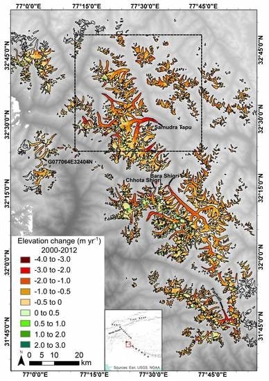
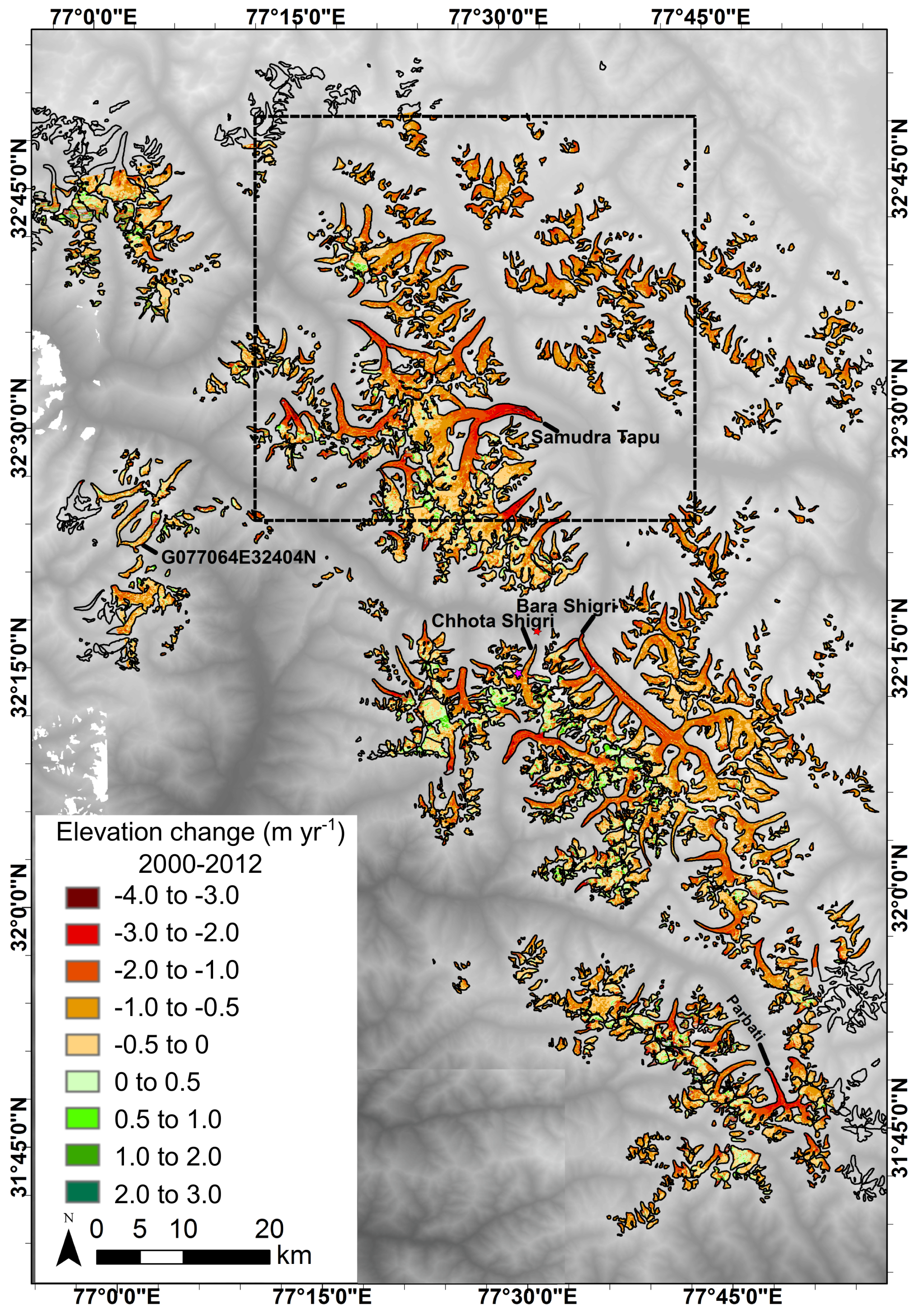
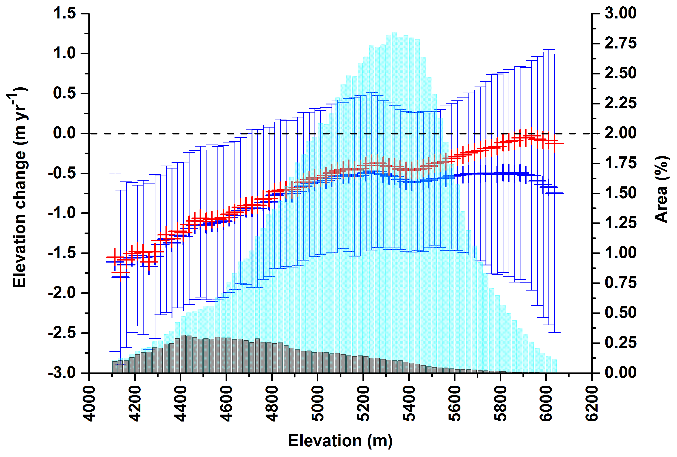
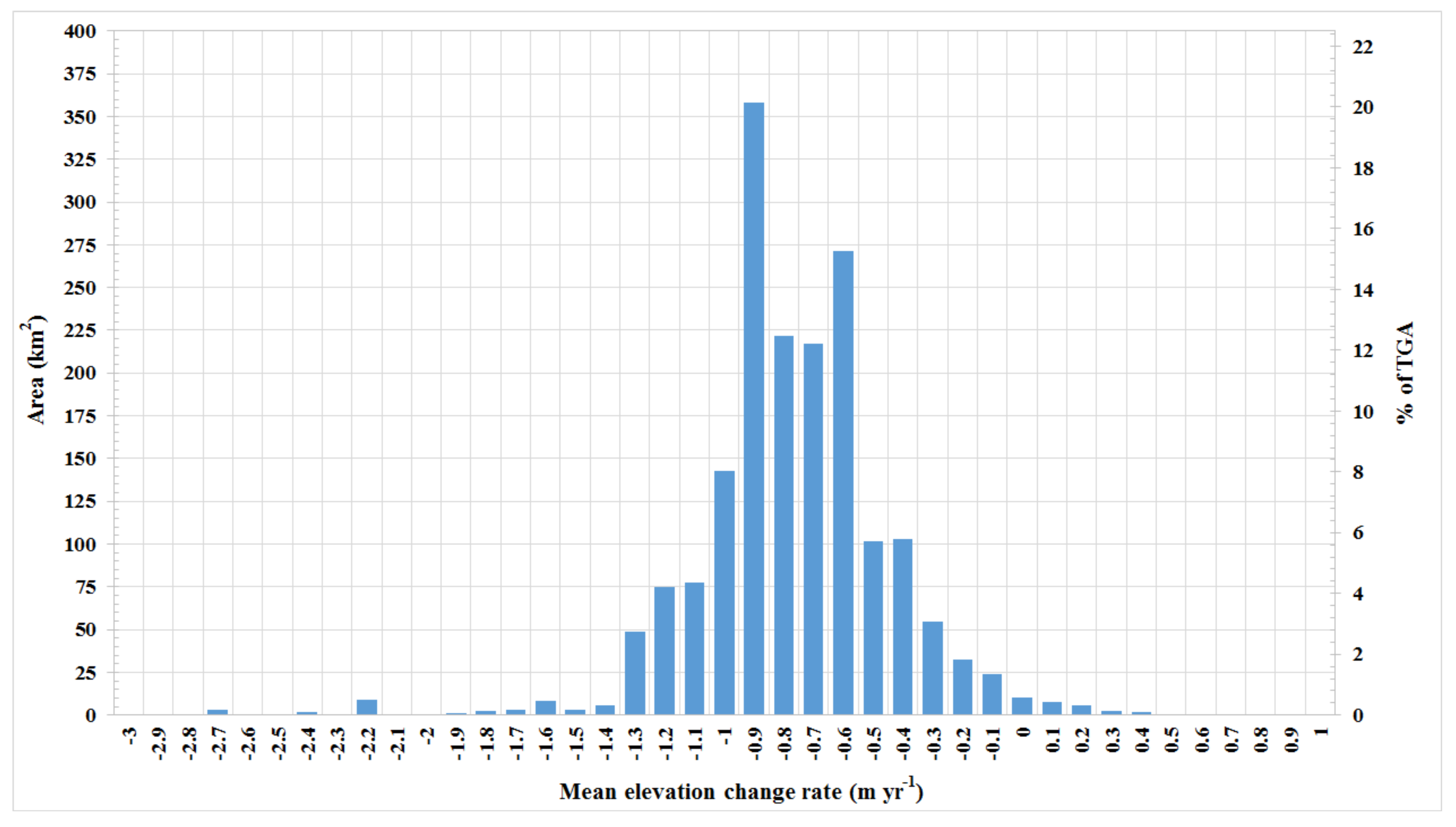
5.2. Mean Glacier Surface Elevation Changes during 2000–2012

We quantified spatially detailed elevation change for 1437 glaciers with a total area of ∼1796.33 km${}^2$ during 2000–2012 (Figure 6). We could observe ∼1712.08 km${}^2$ of glaciated area because of the limited coverage of TanDEM-X data in the north-western and south-eastern sides of the Lahaul-Spiti (Figure 3). As shown in Figure 6, the glaciers have undergone variable elevation change rates in the period of observation. Highest elevation change rates (−3 m yr${}^{-1}$ to −2 m yr${}^{-1}$) were observed for a set of 27 glaciers, which are very small in size ranging from 0.05 km${}^2$ to 1.67 km${}^2$ except $G076996E32414N$ (7.93 km${}^2$). Similarly, ∼84% of 241 glaciers, which showed an elevation change rate of −2 m yr${}^{-1}$ to −1 m yr${}^{-1}$, are small in size (<1 km${}^2$) except a cluster of 3 nearby big glaciers. These glaciers $G077368E32554N$ (29.63 km${}^2$), $G077301E32493N$ (19.19 km${}^2$) and $G077439E32564N$ (14.49 km${}^2$) showed a mean rate of −1.23 m yr${}^{-1}$, −1.17 m yr${}^{-1}$ and −1.11 m yr${}^{-1}$, respectively. The surface elevation of most of the glaciers (∼90% of total areal extent) changed with a rate between −1 m yr${}^{-1}$ and 0 m yr${}^{-1}$. Bara Shigri (110.59 km${}^2$), the biggest glacier of the region, and Chhota Shigri (13.13 km${}^2$), a benchmark glacier, showed a mean elevation change of −0.81 m yr${}^{-1}$ and −0.56 m yr${}^{-1}$, respectively. We observed positive elevation changes for 98 glaciers corresponding to only 1.69% of the glaciated area.

5.3. Geodetic Mass Balance during 2000–2012

Table 2 shows the geodetic mass balance of the entire glacierized area of the Lahaul-Spiti and five selected glaciers during 2000–2012. We observed negative mass budgets at Lahaul-Spiti in the range of −0.52 ± 0.32 m w.e. yr${}^{-1}$ (case C) to −0.58 ± 0.39 m w.e. yr${}^{-1}$ (case A) during 2000–2012 (Table 2). With density assumptions in case B, the mass budget was comparable (−0.53 ± 0.37 m w.e. yr${}^{-1}$) to estimates from case C. Out of the selected glaciers, the most negative mass budget (−0.93 ± 0.37 m w.e. yr${}^{-1}$) was obtained for $G077439E32564N$ (3F in Figure S3). Mass budget estimates of Chhota Shigri and $G077064E32404N$ were less negative in comparison to region-wide mass budgets (Table 2). However, Samudra Tapu, Bara Shigri and Parbati glaciers rapidly lost mass during this period in contrast to region-wide estimates.

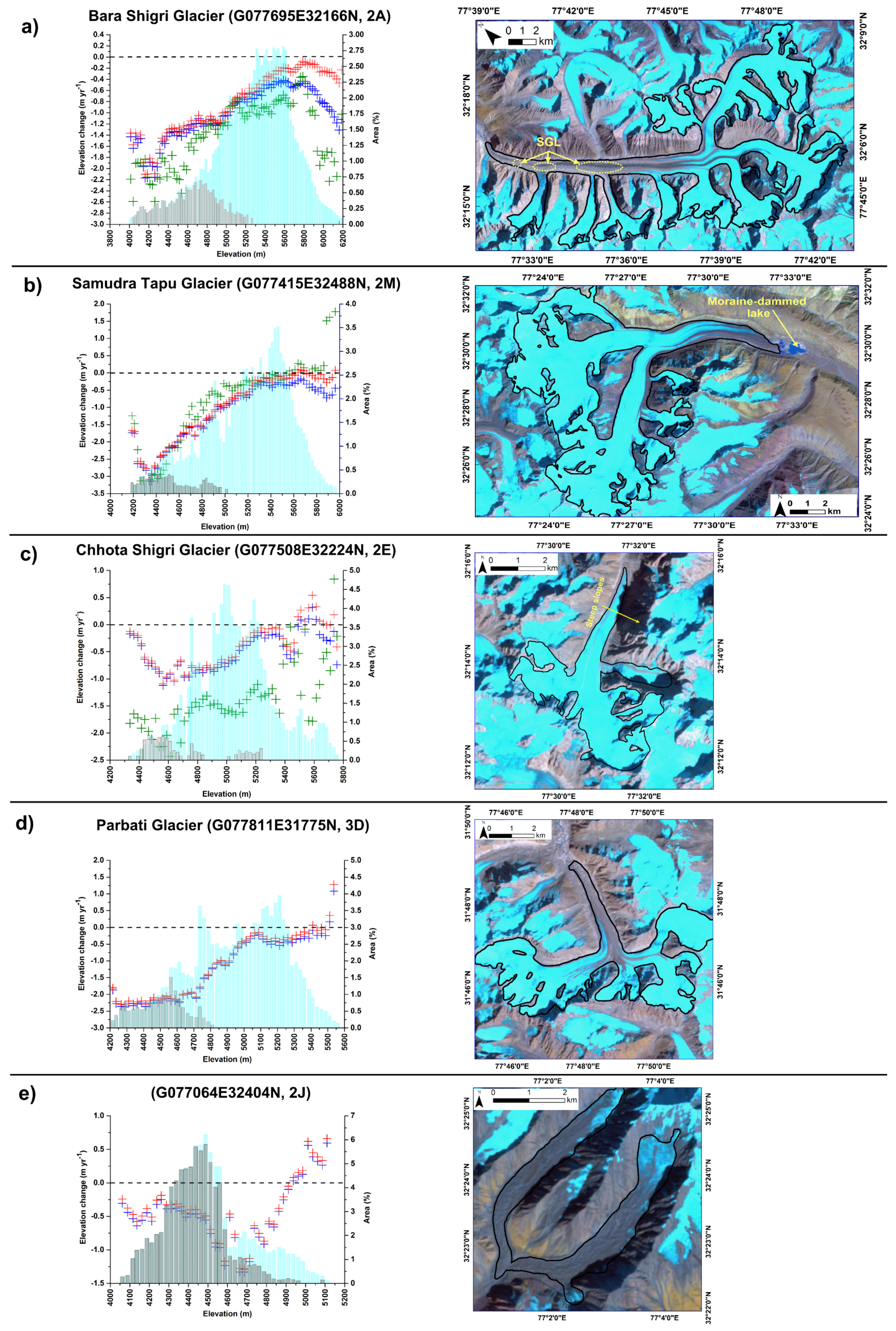
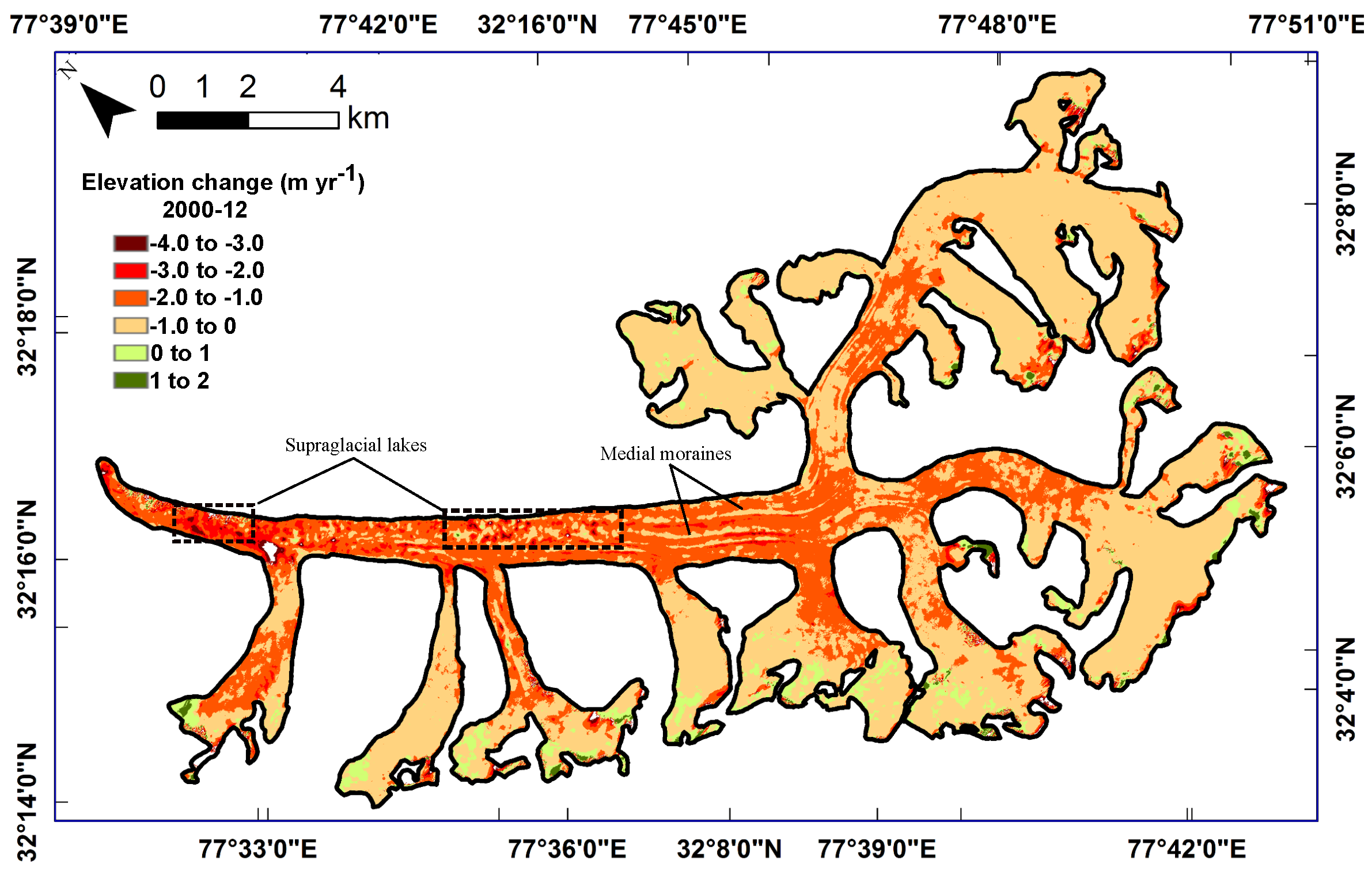
5.4. Spatial Elevation Change Patterns on Glacier Scale during 2000–2012

In order to analyze the spatial patterns of elevation changes on a catchment scale, we performed a hypsometric analysis (glacier bins of 25 m) for 29 glaciers covering at least 8 km${}^2$ of the surface area. These glaciers exhibit different surface and topographic conditions, for example variable extents of supraglacial debris, ponds and lakes, terminus (land- or lake-terminating) etc. We observed three distinct elevation change patterns.

The first pattern (type-1) shows maximum thinning close to the glacier terminus (Figure S4). The surface of type-1 glaciers is only <10% debris-covered (Figure S3). Most of the type-1 glaciers are located at high altitudes with terminus elevations mostly above 4500 m except 1B (∼4300 m) and 1C (∼4000 m). The second pattern (type-2) shows maximum thinning up-glacier instead at the glacier terminus (Figure S5). We found thirteen glaciers which showed type-2 behavior (Figure S3), however, the elevation of maximum thinning from the terminus varies considerably (Figure S5). For example, the point of maximum thinning (−1.33 m yr${}^{-1}$) for G077064E32404N (2J in Figure S5) is located at ∼4686 m in comparison to thinning (−0.30 m yr${}^{-1}$) at its terminus located at ∼4061 m. Most of the type-2 glaciers are highly debris-covered (>10%) with three exceptions 2B (9.75%), 2E (6.06%) and 2I (6.96%). However, thinning increases with a decrease in debris cover extent and achieves its maxima for 2B, 2E and 2I glaciers like for the rest of the type-2 glaciers. In contrast to type-2, several other glaciers with extensive debris-cover (>10%) show strongest surface lowering rates towards the terminus in the debris covered region (Figure S6). We hence separate those in an extra class (type-3).

Lake-terminating glaciers show a mixed elevation change patterns and hence are placed in those categories. For example, the maximum thinning for G077415E32488N (2M, Samudra Tapu Glacier) is located up-glacier (∼4388 m) instead at its terminus (∼4188 m) (Figure S5). In contrary, G077241E32496 (3G) thinned with a maximum rate of −2.70 m yr${}^{-1}$ at the terminus (∼4118 m) (Figure S6). Both lake-terminating glaciers underwent a frontal retreat due to calving into moraine-dammed lakes.

5.5. Elevation and Mass Changes for Selected Glaciers between 2000–2012 and 2012–2013

We measured elevation changes and mass budgets for Samudra Tapu, Bara Shigri and Chhota Shigri glaciers during 2012–2013 where TanDEM-X data was available (Table 2). The hypsometric analysis of elevation changes revealed that the point of maximum thinning during 2012–2013 was nearby or almost similar as from 2000–2012 for all three glaciers (green and blue “+” in Figure 5a–c). However, the magnitude of elevation change differs considerably, especially in case of Bara Shigri and Chhota Shigri. Nearly balanced mass budgets were observed for Samudra Tapu (−0.10 ± 1.29 m w.e. yr${}^{-1}$ with case A) during 2012–2013 but were more negative (−0.72 ± 0.33 m w.e. yr${}^{-1}$) during 2000–2012. Mass budgets were slightly positive for Bara Shigri (−0.55 ± 1.32 m w.e. yr${}^{-1}$) in contrast to the estimates (−0.70 ± 0.33 m w.e. yr${}^{-1}$) during 2000–2012. The mass budget of Chhota Shigri during 2012–2013 was far more negative (−0.91 ± 1.36 m w.e. yr${}^{-1}$) from those observed in 2000–2012 (Table 2). However, it has to be noted that the uncertainties of the 2012–2013 elevation change measurements are high due to the short observation interval.

6. Discussion

6.1. Radar Penetration Bias

The radar signal penetrates into the glacier depending on its surface characteristics (debris-covered ice, clean ice, firn and snow) and surface condition (melt/freeze) inducing a bias in surface elevation measurements [35,36]. During winter conditions, fresh snow is almost transparent for the X- and C-band radar signal and penetration into frozen firn can occur. Surface scattering is dominant in areas of bare ice and hence penetration is low. Similarly, where debris cover is present, scattering is primarily from the surface [28]. Our observations with a strong altitudinal dependency of our SRTM C- and X-band penetration difference showing maximum difference at higher altitudes consisting of dry snow and firn layers confirm these interpretations. During winter conditions [34] also noted C- and X-band penetration difference of 2.90 m over alpine glaciers (370 km${}^2$), which is in the range of our measurements. Previously, Kääb et al. [1] estimated a mean SRTM C-band penetration into debris-covered ice of 0.4 ± 0.8 m, 1.7 ± 0.6 m for clean ice and 2.3 ± 0.6 m for firn/snow in the Lahaul-Spiti and adjacent regions. We expect these values were underestimated as they were computed by temporally extrapolating sparse ICESat observations averaged over large regions and assuming similar glacier elevation changes during 2000−2003 and 2003–2009. In addition, these values, once subtracted from our SRTM C- and X-band penetration difference estimates, would indicate almost zero or even negative values, in some cases, of SRTM X-band penetration depths. This seems inappropriate as the X-band signal can penetrate up to several meters in snow and firn during winter conditions [15]. In contrary to [1], Berthier et al. [34] presented high values of SRTM C-band penetration depth ranging from 0 m to 12 m (altitude dependent) in the Mont-Blanc area of the European Alps.

Our correction assumes a similar penetration of the X-band signals from SRTM and TanDEM-X even though they are 12 years apart. This is certainly limited by the changes in the structure of the snow/firn cover over time and hence the scattering phase centers might be located at slightly different depths. However, there are no field measurements or other means for the respective acquisition dates in order to better quantify this uncertainty. For other regions like the Antarctic Peninsula or the Karakoram, the assumption of comparable penetration depth of X-band radar signals in similar months (or season) has proved to be a suitable approach [24,37,38].

6.2. Geodetic Mass Balance Estimates

Several studies have computed geodetic mass balances of glaciers in high-mountain Asia in different time periods [1,14,39]. In the period 2003–2009, Kääb et al. [1] measured geodetic mass balance of −0.32 ± 0.06 m w.e. yr${}^{-1}$ (Case C density assumption) for glaciers in the Lahaul-Spiti and adjacent regions. Differences in our mass balance estimates (−0.52 ± 0.32 m w.e. yr${}^{-1}$) can be primarily attributed to different periods of observation. In addition, Kääb et al. [1] averaged sparse ICESat observations from adjacent regions (Uttarakhand and West Nepal) with Lahaul-Spiti, but the climate of Uttarakhand and West Nepal is slightly different from Lahaul-Spiti with less influence of the MLW [4]. Gardelle et al. [14] estimated the mass balance of Bara Shigri (−0.48 ± 0.18 m w.e. yr${}^{-1}$), Chhota Shigri (−0.39 ± 0.18 m w.e. yr${}^{-1}$) and the glaciers in Lahaul-Spiti (−0.45 ± 0.14 m w.e. yr${}^{-1}$) during 1999–2011. Our mass balance estimates of Bara Shigri (−0.66 ± 0.31 m w.e. yr${}^{-1}$), Chhota Shigri (−0.46 ± 0.34 m w.e. yr${}^{-1}$) and the entire region (−0.53 ± 0.37 m w.e. yr${}^{-1}$) during 2000–2012 (case B density assumptions in Table 2) are slightly more negative than theirs even though the period of observations are almost the same. Gardelle et al. [14] used SRTM C-band and SPOT5 DEMs for their elevation change and mass balance estimates. In order to correct the bias due to the C-band radar signal penetration, they subtracted SRTM X- and C-band elevations, while assuming no penetration of X-band signal into glacier. This assumption has already been challenged by [15] who observed 4-6 m of X-band penetration depth under winter conditions (February) in the Mont-Blanc area in the European Alps. Berthier et al. [34] also highlighted this fact and approximated at least 5 to 6 m of X-band penetration in the Mont-Blanc area. Moreover, Gardelle et al. [14] corrected the C-band penetration depth for Lahaul-Spiti region using the observations in Karakoram where the surface and snow/firn condition of glaciers might not be the same. Our results suggest that the glaciers in Lahaul-Spiti appear to be losing mass more rapidly compared to the Karakoram glaciers as observed by [24] using similar data, methods and observation period like in the present study. This is in line with the overall known picture of the so-called “Karakoram anomaly” and the ICESat analysis by [1] for entire high-mountain Asia.

6.3. Heterogeneous Elevation Change Patterns and Possible Reasons

The increasing thinning rates towards glacier terminus of type-1 glaciers can be explained by the higher air temperatures at lower elevations and lower albedo of the bare ice compared to the snow and firn covered areas. For type-2 glaciers the insulating effect of a thick debris-cover is considered to be the probable reason for the reduced melt. Down-glacier areas are prone to have thicker debris compared to up-glacier because of avalanche driven debris from steep areas and the emergence of englacial debris [40]. Consequently, maximum thinning takes place at higher altitudes, where either comparably thinner debris cover or supraglacial ponds and lakes, and ice-cliffs trigger lowering [7]. Dobhal et al. [12] also observed ∼4 times higher melt rates at 4400 m compared to the terminus (∼3900 m) of Chorabari Glacier in Indian Himalaya and linked this to the insulating effects of thick debris cover at lower altitudes.

Dobhal et al. [1] showed similar thinning rates of debris-covered ice and clean ice in high- mountain Asia during 2003–2008. Gardelle et al. [14] seconded this for Lahaul-Spiti region by differencing SRTM C-band and SPOT5 DEMs during 1999–2011. In both cases, the measurements were averaged over large areas and do not show large scale thinning patterns due to several counteracting processes in debris-covered region. To validate this point, we present a case study of Bara Shigri Glacier (Figure 5a ) which has supraglacial debris (18.43%) and lakes and several ice cliffs. The surface elevation change rate (2000–2012) of Bara Shigri indicates spatially variable thinning patterns on its surface (Figure 7). Very high rates (−3 m yr${}^{-1}$ to −2 m yr${}^{-1}$) of lowering can be observed at or nearby supraglacial lakes. Higher thinning rates (−2 m yr${}^{-1}$ to −1 m yr${}^{-1}$) can also be detected over exposed ice in comparison to nearby ice covered with medial moraines (−1 m yr${}^{-1}$ to 0 m yr${}^{-1}$). We expect that supraglacial lakes and exposed ice absorb more solar radiation and foster thinning. In contrary, the debris of the medial moraines protects the ice beneath from melting. These counteracting processes take place in close proximity. Our analysis with smaller glacier bins (25 m) reveals the large-scale patterns of glacier elevation change possibly driven by above-mentioned counteracting processes. We do not have adequate information of debris thickness for our studied glaciers, however, Schauwecker et al. [13] recently estimated debris thickness of Bara Shigri Glacier using an energy-balance approach. They showed spatially variable debris thickness over its surface which reaches up to 30 cm at down-glacier areas and lateral margins [13]. Unfortunately this approach might also underestimate debris thickness due to the unknown vertical temperature profile and heat exchange through the debris layer [13]. Therefore we cannot completely rely on their measurements to verify our hypothesis.

Several other glaciers show type-3 behaviour (extensive debris-cover (>10%), highest lowering near the terminus) in our dataset. These glaciers consist of several supraglacial lakes, ponds and ice cliffs in the debris-covered areas. For instance, $G077811E31775N$ (3D, Parbati glacier), $G077606E32140N$ (3A) and $G077633E32112N$ (3C) (Figure S3) have many supraglacial lakes and ice cliffs at their lower reaches, but $G077559E32106N$ (3E) has supraglacial lakes even at higher altitudes (∼5000 m). $G077368E32554N$ (3B), $G077439E32564N$ (3F) and $G077241E32496$ (3G) have several ice cliffs. These supraglacial features cannot be mapped with Landsat-7 ETM or Landsat-8 OLI, however, we could detect them using high-resolution Google Earth images. Two different mechanisms can be responsible for type-3 pattern. One reason could be that the debris-cover is not thick enough to fully protect the ice from melting, but thick enough to reveal a spectral debris-cover signature in the Landsat imagery. A second explanation is that a thick debris cover reduces ice melt [6,12] while ice-cliff ablation [10], melting of ice beneath supraglacial ponds and lakes can foster ice melt [11]. Ice cliffs may absorb 10 times more heat than the debris covered areas [9] and foster ablation even though their spatial extent is comparably small [10]. For instance, Sakai et al. [41] noted 20% of ice cliff ablation despite they account for about 2% of entire debris-covered part of Lirung Glacier, Nepal Himalaya. Nuimura et al. [23] also highlighted the dominant effect of ice cliff ablation over debris covered areas in Khumbu region, Nepal Himalaya. This combined effect could be enough to explain the observed pattern.

7. Conclusions and Outlook

This study presents region-wide and glacier-specific elevation change and geodetic mass balance observations derived from SRTM C-/X-band and TanDEM-X DEMs during 2000–2012 and 2012–2013. Our study provides a complete methodological framework to use bistatic TanDEM-X and SRTM C-/X-band data for accurate and detailed mapping of elevation change and mass balance estimates. This framework can be further replicated for different study regions as the TanDEM-X data has a global coverage. We suggest large time intervals of TanDEM-X repeat acquisition under similar surface conditions are needed to reduce errors. This study also demonstrates the importance to correct for radar signal penetration into different surface types when using SRTM C-band DEM and other radar frequencies (e.g., X-band of TanDEM-X) or optical data. We show that this bias, if not removed, can deteriorate geodetic mass balance estimates by as high as 20% like in this study.

Contrary to the generalized conclusions, by [1,14], that the debris-covered and debris-free ice have similar thinning patterns in several regions of high-mountain Asia, we found two different thinning patterns for debris-covered glaciers. We conclude that the maximum thinning might occur up-glacier for debris-covered glaciers with a thick insulating debris cover (type-2). However, maximum thinning might also take place at or near the terminus (type-3) due to less thick debris-cover or enhanced melting from supraglacial lakes, ponds and ice cliffs. Therefore, we suggest high resolution datasets and observations of individual glaciers should be employed to overcome such averaging effects. Future work should emphasize on the precise measurements of debris thickness, spatial extents of ice cliffs and supraglacial water bodies. This further leads to determine to what degree the counteracting forces on debris-covered glaciers dominate each other and influence the glacier response to climate. More studies on radar signal penetration of different frequencies under different surface conditions are required for a better assessment of resulting uncertainties in glacier elevation and mass change computations.

References

1. Kääb, A.; Berthier, E.; Nuth, C.; Gardelle, J.; Arnaud, Y. Contrasting patterns of early twenty-first-century glacier mass change in the Himalayas. Nature 2012, 488, 495–498. [Google Scholar] [CrossRef] [PubMed]
2. Azam, M.F.; Wagnon, P.; Vincent, C.; Ramanathan, A.; Favier, V.; Mandal, A.; Pottakkal, J.G. Processes governing the mass balance of Chhota Shigri Glacier (western Himalaya, India) assessed by point-scale surface energy balance measurements. Cryosphere 2014, 8, 2195–2217. [Google Scholar] [CrossRef]
3. Singh, S.; Kumar, R.; Bhardwaj, A.; Sam, L.; Shekhar, M.; Singh, A.; Kumar, R.; Gupta, A. Changing climate and glacio-hydrology in Indian Himalayan Region: A review. Wiley Interdiscip. Rev. Clim. Chang. 2016, 7, 393–410. [Google Scholar]
4. Wiltshire, A.J. Climate change implications for the glaciers of the Hindu Kush, Karakoram and Himalayan region. Cryosphere 2014, 8, 941–958. [Google Scholar] [CrossRef]
5. Vincent, C.; Ramanathan, A.; Wagnon, P.; Dobhal, D.P.; Linda, A.; Berthier, E.; Sharma, P.; Arnaud, Y.; Azam, M.F.; Jose, P.G.; et al. Balanced conditions or slight mass gain of glaciers in the Lahaul and Spiti region (northern India, Himalaya) during the nineties preceded recent mass loss. Cryosphere 2013, 7, 569–582. [Google Scholar] [CrossRef] [Green Version]
6. Anderson, L.S.; Anderson, R.S. Modeling debris-covered glaciers: response to steady debris deposition. Cryosphere 2016, 10, 1105–1124. [Google Scholar] [CrossRef]
7. Ragettli, S.; Bolch, T.; Pellicciotti, F. Heterogeneous glacier thinning patterns over the last 40 years in Langtang Himal, Nepal. Cryosphere 2016, 10, 2075–2097. [Google Scholar] [CrossRef]
8. Vincent, C.; Wagnon, P.; Shea, J.M.; Immerzel, W.W.; Kraaijenbrink, P.D.A.; Shrestha, D.; Soruco, A.; Arnaud, Y.; Brun, F.; Berthier, E.; et al. Reduced melt on debris-covered glaciers: Investigations from Changri Nup Glacier, Nepal. Cryosphere 2016, 10, 1845–1858. [Google Scholar] [CrossRef] [Green Version]
9. Sakai, A.; Takeuchi, N.; Fujita, K.; Nakawo, M. Role of supraglacial ponds in the ablation process of a debris-covered glacier in the Nepal Himalayas. In Debris-Covered Glaciers; IAHS Publications: Wallingford, UK, 2000; Volume 265, pp. 119–130. [Google Scholar]
10. Reid, T.; Brock, B. Assessing ice-cliff backwasting and its contribution to total ablation of debris-covered Miage glacier, Mont Blanc massif, Italy. J. Glaciol. 2014, 60, 3–13. [Google Scholar] [CrossRef]
11. Benn, D.I.; Bolch, T.; Hands, K.; Gulley, J.; Luckman, A.; Nicholson, L.I.; Quincey, D.; Thompson, S.; Toumi, R.; Wiseman, S. Response of debris-covered glaciers in the Mount Everest region to recent warming, and implications for outburst flood hazards. Earth-Sci. Rev. 2012, 114, 156–174. [Google Scholar] [CrossRef] [Green Version]
12. Dobhal, D.; Mehta, M.; Srivastava, D. Influence of debris cover on terminus retreat and mass changes of Chorabari Glacier, Garhwal region, central Himalaya, India. J. Glaciol. 2013, 59, 961–971. [Google Scholar] [CrossRef]
13. Schauwecker, S.; Rohrer, M.; Huggel, C.; Kulkarni, A.; Ramanathan, A.L.; Salzmann, N.; Stoffel, M.; Brock, B. Remotely sensed debris thickness mapping of Bara Shigri Glacier, Indian Himalaya. J. Glaciol. 2015, 61, 675–688. [Google Scholar] [CrossRef]
14. Gardelle, J.; Berthier, E.; Arnaud, Y.; Kääb, A. Region-wide glacier mass balances over the Pamir-Karakoram- Himalaya during 1999–2011. Cryosphere 2013, 7, 1263–1286. [Google Scholar] [CrossRef] [Green Version]
15. Dehecq, A.; Millan, R.; Berthier, E.; Gourmelen, N.; Trouvé, E.; Vionnet, V. Elevation changes inferred from TanDEM-X data over the Mont-Blanc area: Impact of the X-band interferometric Bias. IEEE J. Sel. Top. Appl. Earth Observ. Remote Sens. 2016, 9, 3870–3882. [Google Scholar] [CrossRef]
16. Rott, H.; Yueh, S.H.; Cline, D.W.; Duguay, C.; Essery, R.; Haas, C.; Heliere, F.; Kern, M.; Macelloni, G.; Malnes, E.; et al. Cold Regions hydrology high-resolution observatory for snow and cold land processes. Proc. IEEE 2010, 98, 752–765. [Google Scholar] [CrossRef] [Green Version]
17. Wagnon, P.; Linda, A.; Arnaud, Y.; Kumar, R.; Sharma, P.; Vincent, C.; Pottakkal, J.G.; Berthier, E.; Ramanathan, A.; Hasnain, S.I.; et al. Four years of mass balance on Chhota Shigri Glacier, Himachal Pradesh, India, a new benchmark glacier in the western Himalaya. J. Glaciol. 2007, 53, 603–611. [Google Scholar] [CrossRef]
18. Azam, M.F.; Ramanathan, A.; Wagnon, P.; Vincent, C.; Linda, A.; Berthier, E.; Sharma, P.; Mandal, A.; Angchuk, T.; Singh, V.B.; et al. Meteorological conditions, seasonal and annual mass balances of Chhota Shigri Glacier, western Himalaya, India. Ann. Glaciol. 2016, 57, 328–338. [Google Scholar] [CrossRef]
19. Azam, M.F.; Wagnon, P.; Vincent, C.; Ramanathan, A.; Linda, A.; Singh, V.B. Reconstruction of the annual mass balance of Chhota Shigri glacier, Western Himalaya, India, since 1969. Ann. Glaciol. 2014, 55, 69–80. [Google Scholar] [CrossRef]
20. Hoffmann, J.; Walter, D. How Complementary are SRTM-X and C-Band digital elevation models? Photogramm. Eng. Remote Sens. 2006, 72, 261–268. [Google Scholar] [CrossRef]
21. Krieger, G.; Moreira, A.; Fiedler, H.; Hajnsek, I.; Werner, M.; Younis, M.; Zink, M. TanDEM-X: A satellite formation for high-resolution SAR interferometry. IEEE Trans. Geosci. Remote Sens. 2007, 45, 3317–3341. [Google Scholar] [CrossRef]
22. Arendt, A.; Bliss, A.; Bolch, T.; Cogley, J.G.; Gardner, A.S.; Hagen, J.O.; Hock, R.; Huss, M.; Kaser, G.; Kienholz, C.; et al. Randolph Glacier Inventory—A Dataset of Global Glacier Outlines: Version 5.0; Technical Report; Global Land Ice Measurements from Space: Boulder, CO, USA, 2015. [Google Scholar]
23. Nuimura, T.; Sakai, A.; Taniguchi, K.; Nagai, H.; Lamsal, D.; Tsutaki, S.; Kozawa, A.; Hoshina, Y.; Takenaka, S.; Omiya, S.; et al. The GAMDAM glacier inventory: A quality-controlled inventory of Asian glaciers. Cryosphere 2015, 9, 849–864. [Google Scholar] [CrossRef]
24. Rankl, M.; Braun, M. Glacier elevation and mass changes over the central Karakoram region estimated from TanDEM-X and SRTM/X-SAR digital elevation models. Ann. Glaciol. 2016, 51, 273–281. [Google Scholar] [CrossRef]
25. Rosen, P.A.; Werner, C.W.; Hiramatsu, A. Two-dimensional phase unwrapping of SAR interferograms by charge connection through neutral trees. In Proceedings of the Geoscience and Remote Sensing Symposium (IGARSS), Pasadena, CA, USA, 8–12 August 1994.
26. Costantini, M. A novel phase unwrapping method based on network programming. IEEE Trans. Geosci. Remote Sens. 1998, 36, 813–821. [Google Scholar] [CrossRef]
27. Fritz, T.; Rossi, C.; Yague-Martinez, N.; Rodriguez-Gonzalez, F.; Lachaise, M.; Breit, H. Interferometric processing of TanDEM-X data. In Proceedings of the Geoscience and Remote Sensing Symposium (IGARSS), Vancouver, BC, Canada, 24–29 July 2011.
28. Gardelle, J.; Berthier, E.; Arnaud, Y. Impact of resolution and radar penetration on glacier elevation changes computed from DEM differencing. J. Glaciol. 2012, 58, 419–422. [Google Scholar] [CrossRef]
29. Huss, M. Density assumptions for converting geodetic glacier volume change to mass change. Cryosphere 2013, 7, 877–887. [Google Scholar] [CrossRef]
30. Guo, Z.; Wang, N.; Kehrwald, N.M.; Mao, R.; Wu, H.; Wu, Y.; Jiang, X. Temporal and spatial changes in Western Himalayan firn line altitudes from 1998 to 2009. Glob. Planet. Chang. 2014, 118, 97–105. [Google Scholar] [CrossRef]
31. Dormann, C.F.; McPherson, J.M.; Araújo, M.B.; Bivand, R.; Bolliger, J.; Carl, G.; Davies, R.G.; Hirzel, A.; Jetz, W.; Kissling, W.D.; et al. Methods to account for spatial autocorrelation in the analysis of species distributional data: A review. Ecography 2007, 30, 609–628. [Google Scholar] [CrossRef]
32. Höhle, J.; Höhle, M. Accuracy assessment of digital elevation models by means of robust statistical methods. ISPRS J. Photogramm. Remote Sens. 2009, 64, 398–406. [Google Scholar] [CrossRef]
33. Holzer, N.; Vijay, S.; Yao, T.; Xu, B.; Buchroithner, M.; Bolch, T. Four decades of glacier variations at Muztagh Ata (eastern Pamir): A multi-sensor study including Hexagon KH-9 and Pléiades data. Cryosphere 2015, 9, 2071–2088. [Google Scholar] [CrossRef]
34. Berthier, E.; Cabot, V.; Vincent, C.; Six, D. Decadal region-wide and glacier-wide mass balances derived from multi-temporal ASTER satellite digital elevation models. Validation over the Mont-Blanc area. Front. Earth Sci. 2016, 4, 63. [Google Scholar] [CrossRef]
35. Mätzler, C. Applications of the interaction of microwaves with the natural snow cover. Remote Sens. Rev. 1987, 2, 259–387. [Google Scholar] [CrossRef]
36. Müller, K.; Hamran, S.E.; Sinisalo, A.; Hagen, J.O. Phase center of L- band radar in polar snow and ice. IEEE Trans. Geosci. Remote Sens. 2011, 49, 4572–4579. [Google Scholar] [CrossRef]
37. Rott, H.; Floricioiu, D.; Wuite, J.; Scheiblauer, S.; Nagler, T.; Kern, M. Mass changes of outlet glaciers along the Nordensjköld Coast, northern Antarctic Peninsula, based on TanDEM-X satellite measurements. Geophys. Res. Lett. 2014, 41, 8123–8129. [Google Scholar] [CrossRef]
38. Seehaus, T.; Marinsek, S.; Helm, V.; Skvarca, P.; Braun, M. Changes in ice dynamics, elevation and mass discharge of Dinsmoor-Bombardier-Edgeworth glacier system, Antarctic Peninsula. Earth Planet. Sci. Lett. 2015, 427, 125–135. [Google Scholar] [CrossRef]
39. Nuimura, T.; Fujita, K.; Yamaguchi, S.; Sharma, R.R. Elevation changes of glaciers revealed by multitemporal digital elevation models calibrated by GPS survey in the Khumbu region, Nepal Himalaya, 1992–2008. J. Glaciol. 2012, 58, 648–656. [Google Scholar] [CrossRef]
40. Basnett, S.; Kulkarni, A.V.; Bolch, T. The influence of debris cover and glacial lakes on the recession of glaciers in Sikkim Himalaya, India. J. Glaciol. 2013, 59, 1035–1046. [Google Scholar] [CrossRef] [Green Version]
41. Sakai, A.; Nakawo, M.; Fujita, K. Distribution characteristics and energy balance of ice cliffs on debris-covered laciers, Nepal Himalaya. Arct. Antarct. Alp. Res. 2002, 34, 12–19. [Google Scholar] [CrossRef]
Figure 1. Map of the mountain ranges of high-mountain Asia showing the major rivers (light blue polylines) and two wind systems (MLW and ISM). The blue rectangle represents the study region (Lahaul-Spiti).
Remotesensing 08 01038 g001
Figure 2. Hypsometric plot of the observed SRTM C- and X- band penetration difference (SRTM-X elevation minus SRTM-C elevations) (red dots) over clean ice/firn/snow in the area represented by a black dashed rectangle in Figure 3. These observations are exponentially fit (black dotted) with a function y = 7E-06e 0.0023 x and R 2 value of 0.94. Here, (y) represents the SRTM C- and X-band penetration difference over clean ice/firn/snow and (x) is the elevation. Blue columns show the corresponding area (km 2 ) where X- and C- band penetration differences are observed.
Remotesensing 08 01038 g002
Figure 3. Map of elevation changes of glaciers in the Lahaul-Spiti region between February 2000 and Januray–February 2012. The black dotted rectangle indicates the area where SRTM C- and X- band penetration difference was calculated.
Remotesensing 08 01038 g003
Figure 4. Hypsometric elevation change plot of the observed glaciated area of Lahaul-Spiti region (∼1712 km 2 ) using 25 m elevation bins. The cyan and gray columns show the fraction of total glaciated area and debris covered area in the corresponding bins. The blue “+” and 2D range plots show the median and ±NMAD elevation change (2000–2012) respectively in the corresponding bins after correcting the C- and X- band penetration bias. The red “+” indicate the uncorrected median elevation change.
Remotesensing 08 01038 g004
Figure 5. The left and right panel show the hypsometric elevation change plots and the catchments of (a) Bara Shigri, (b) Samudra Tapu, (c) Chhota Shigri, (d) Parbati and (e) G 077064 E 32404 N glaciers. The cyan and gray columns show the fractions of total glaciated area and debris covered area in the corresponding bins. The surface of Bara Shigri is covered by several supraglacial lakes, few of them indicated as SGL in (a). The blue “+” in the plots represent the median elevation change (2000–2012) in the corresponding bins after correcting for the C- and X- band penetration bias. The red “+” indicate the uncorrected median elevation change during 2000–2012. Green “+” represent the median elevation change during 2012–2013.
Remotesensing 08 01038 g005
Figure 6. Mean elevation change rate (m yr 1 ) of 1437 glaciers in the Lahaul-Spiti during 2000–2012 is represented by x-axis. The two y axes represent the catchment area (left y-axis) of the observed glaciers and the proportion of total glaciated area (TGA) covered by their catchment (right y-axis).
Remotesensing 08 01038 g006
Figure 7. Elevation change map of Bara Shigri Glacier during 2000–2012. The location of few supraglacial lakes and medial moraines are indicated.
Remotesensing 08 01038 g007