Estimation of Building Density with the Integrated Use of GF-1 PMS and Radarsat-2 Data

Abstract

Building density, as a component of impervious surface fraction, is a significant indicator of population distribution as essentially all humans live and conduct activities in buildings. Because population spatialization usually occurs over large areas, large-scale building density estimation through a proper, time-efficient, and relatively precise way is urgently required. Therefore, this study constructed a decision tree by the Classification and Regression Tree (CART) algorithm combining synthetic aperture radar (SAR) with optical images. The input features included four spectral bands (B_1–4) of GF-1 PMS imagery; Normalized Difference Vegetation Index (NDVI), Normalized Difference Water Index (NDWI), and Ratio Built-up Index (RBI) derived from them; and backscatter intensity (BI) of Radarsat-2 SAR data. In addition, a new index called amended backscatter intensity (ABI), which takes the influence created by different spatial patterns into account, was introduced and calculated through fractal dimension and lacunarity. Result showed that before the integration use of multisource data, a model using B_1–4, NDVI, NDWI, and RBI had the highest accuracy, with RMSE of 10.28 and R² of 0.63 for Jizhou and RMSE of 20.34 and R² of 0.36 for Beijing. In Comparison, the best model after combining two data sources (i.e., the model employing B_1–4, NDVI, NDWI, RBI and ABI) reduced the RMSE to 8.93 and 16.21 raised the R² to 0.80 and 0.64, respectively. The result indicated that the synergistic use of optical and SAR data has the potential to improve the building density estimation performance and the addition of ABI has a better capacity for improving the model than other input features.

1. Introduction

Population distribution is an extremely complicated function of regional character; therefore, a precise description of spatial population distribution is essential to support planning processes such as the design of public and private facilities and the study of urbanization and population changes as well as the relationship between human activities and environmental changes [1,2].

The impervious surface percentage (ISP), which indicates the percentage of impervious surface over an area, contains the most robust information about housing density and the stage of housing construction [1]. It is particularly attractive because it requires no a priori knowledge of land cover [3]; as a result, the ISP has been employed widely in spatial estimation of population distribution. The most important step in the estimation process involves selecting an appropriate methodology to extract ISP, which has been the subject of extensive studies. Algorithms estimating ISP include linear regression analysis [4,5], classification and regression tree (CART) [3,6,7], spectral mixture analysis (SMA) [1,8], and linear spectral mixture analysis (LMSA) [9]. In addition to research using optical imagery, a combination of optical and SAR data also showed excellent potential to make up for optical images’ inability to distinguish diverse materials, seasonal variation, and cloud coverage [10,11,12,13,14,15,16].

However, by definition, impervious surface refers to any material of natural or anthropogenic origin that prevents the infiltration of water into the soil and thereby changes the flow dynamics, sedimentation load, and pollution profile of storm water runoff [17]. Therefore, impervious surface can reflect terrain that should not be associated with populations (e.g., roads, parking lots, and parks). Schueler [18] divided impervious surface into two parts: rooftops under which people live, work, and shop and the transport system that people use to get from one roof to another. Obviously, percentage of the first part, which can be generalized as building density, should be viewed as a key factor in population estimation.

As a component of ISP, building density is difficult to be extracted since buildings share the same spectral signature with other impervious objects, which leads to the fact that methodologies related to spectral characteristics (e.g., SMA, LSMA, or some per-pixel classifiers) are unsuitable for building density estimation. Thus, commonly used methods to extract building density mainly include automatic building detection and regression modeling.

Automatic detection means automatically extracting buildings by algorithms and obtaining building density by dividing the total area of that region. For example, Li [19] estimated the building density distribution of Yuzhong district in Chongqing using the spectral values of four bands of Quickbird images (0.61 m), shape indices, and a nearest distance algorithm and calculated the floor area ratio based on it in 2007. Yu [20] used a threshold segmentation based on a normalized DSM generated by LiDAR data (0.44 point/m²) to extract buildings in 2010. Wu [21] estimated the building density distribution of Wuhan from TerraSAR-X images (1.25 m) through threshold segmentation and corrected it with a least squares fitting method in 2011 and Cao [22] improved the algorithm by bi-threshold and morphological operators with the same sensor data and the same study area in 2012. Kajimoto [23] improved the classification result by correcting the polarization orientation angle (POA) using ALOS/PALSAR data (24 m) and estimated the relative building-to-land ratio (building density) in 2013. Susaki [24], in 2014, extended Kajimoto’s method to multiple PolSAR images and made a comparison of building densities among different cities in.

Regression modeling uses factors theoretically relating to building density (i.e., light intensity in DMSP/OLS imagery and greenness from tasseled cap transformation) to develop a regression model between them and building density. Martin [25] presented an approach for estimating building density on the city block scale by utilizing first-order statistics and co-occurrence texture measure through random forest with TerraSAR-X image (3.07 m × 3.04 m) in 2010. Zheng [26] developed a linear regression model between light intensities of Visible Infrared Imaging Radiometer Suite (VIIRS) images (500 m) and building densities obtained from Google Earth and applied it to eight districts of Nanjing in 2014.

It seems that most previous studies on building density preferred to extract buildings in a certain area (e.g., a city or its center business district) since it might be more precise. However, the drawback is that it requires high-resolution imagery to avoid mixed pixels and to conduct complex analysis of buildings’ characteristics. Therefore, such time-consuming automatic extractions are unsuitable for large areas. There are only a few studies focusing on regression modeling, which does not strictly demand high-resolution imagery and is available in any scale. Regression modeling is simpler and more suitable for implementing over large areas but might be considered imprecise, as statistically related features are not sufficient to display the real distribution of building density. However, proper estimation of population distribution requires a large-extent estimation of building density, which exactly matches to the utility of regression modeling. Thus, appropriate regression algorithms and features are on request to guarantee both extent and precision.

Optical images can provide rich spectral information but are up against a challenge that the diversity of urban land covers will lead to difficulties in separating different land covers with similar spectral signatures [10,11,12,13,16] while SAR images are sensitive to the geometric characteristics of urban land surfaces although they are short of bands [10]. Nevertheless, previous studies related to regression modeling have never synergistically used multi-sensor and multi-satellite data source (e.g., Martin’s TerraSAR-X and Zheng’s VIIRS). Therefore, combination of the optical and SAR data should be fully considered to foster strengths and compensate for weaknesses. Besides, new features are required to directly and precisely reflect building density instead of heuristically trying existed parameters.

Therefore, the objective of this study is to discover a new angle to solving building density estimation from the integration of SAR and optical images as well as a new feature closely relating to building density. To achieve this, two Radarsat-2 images and several GF-1 PMS images of two study areas with different landscapes were employed and a Classification and Regression Tree (CART)-based approach was used to evaluate the feasibility and efficiency of estimating building density ascribing to its success in many previous studies [3,6,7,11].

2. Study Area and Data

2.1. Study Area

The Jing-Jin-Ji urban agglomeration, located in the eastern part of the North China Plain, belongs to the Bohai rim and consists of 10 major cities and several very small cities [27]. Two areas were selected for the study case examples due to their completely disparate urban morphology and building types. Jizhou and the rural settlements around it represent small-scale cities and towns that are in general predominated by traditional building styles (i.e., regularly shaped, closely distributed, flat-roofed, and 6–8 floors high). In a contrast, Beijing is a typical megacity with an unprecedented urbanization rate. In addition to traditional buildings and cultural sloping-roofed courtyard houses, it also has irregular-looking skyscrapers and modern garden-like communities all over the city. Besides, the functional areas of Beijing, including the commercial center, convention center, and opera house, show a more diverse structure. On the whole, the differences between these two regions can be a good evaluation of the new approach’s robustness and universality. Study areas are displayed in Figure 1.

2.2. Data

Two Radarsat-2 images were employed. The one for Jizhou was obtained on 25 April 2015 with a resolution of 4.73 m in range, 4.74 m in azimuth, and an incidence angle of 26.65°. The one for Beijing was obtained on 16 February 2015 with a resolution of 9.14 m in range, 5.18 m in azimuth, and an incidence angle of 31.19°. The pass directions are descending and ascending for Jizhou and Beijing, respectively. According to Franceschetti [28], the dominant return is wall-ground double scattering from buildings when using cross-polarization channels, so we choose the VH band. Image preprocessing including multi-looking, frost filtering, geocoding, orthorectification, and radiometric calibration were conducted by SARscape plugin in ENVI software and the images were finally resampled to 10 m resolution and output in dB format.

As for optical images, ten GF-1 PMS images were downloaded from the Resource and Satellite Center, China (http://www.cresda.com/CN/), and spliced to cover the two regions. GF-1 PMS image has four multispectral bands in the visible and near infrared ranges (0.45–0.52 μm, 0.52–0.59 μm, 0.63–0.69 μm and 0.77–0.89 μm) with 8 m resolution and one panchromatic band (0.45–0.90 μm) with 2 m resolution. GF-1 is a satellite independently-created by China which was launched in recent years, thus, a profound significance exists in research using its imagery. Radiometric calibration, atmospheric correction, and orthorectification were conducted and DN value was eventually converted to at-satellite reflectance. To guarantee the quality of the images, cloud coverage should be less than one percent and the acquisition time images meeting that requirement span several months.

Finally, Google Map images of 0.5 m resolution acquired in August 2015 and February 2015 were used for developing training, validation, and testing datasets.

Each scene was projected to UTM (zone 50) coordinates. The geometric error is less than one Radarsat pixel after registration.

Table 1. Data sources.

Satellite	Path	Row	Obtained Date
Radarsat-2	\	\	25 April 2015
Radarsat-2	\	\	19 February 2015
GF-1	2	92	16 August 2015
GF-1	2	93	16 August 2015
GF-1	2	92	28 August 2015
GF-1	2	92	12 October 2015
GF-1	2	93	12 October 2015
GF-1	1	89	22 January 2015
GF-1	1	89	03 January 2015
GF-1	1	89	15 February 2015
GF-1	2	89	22 January 2015
GF-1	2	89	03 January 2015
Google Map	\	\	11 March 2015
Google Map	\	\	07 August 2015

shows the main data used in this study.

3. Method

A CART-based approach was used to estimate the building density. Google Map high-resolution images provided the reference building density data for training, validation, and testing while the medium-resolution Radarsat-2 and GF-1 PMS imagery were used for mapping building density over a large area. The CART algorithm, which can handle multisource and multisensor data with different statistical distribution and physical parameters, was first used by Yang [6] for ISP estimation. In general, the CART algorithm conducts a binary recursive partitioning process which splits each parent node into two child nodes and then repeats the process by treating each child node as a potential parent node [29]. The advantage of CART algorithm is to simplify complicated non-linear relationship between predictive and target variables into a multivariate linear relation and to continuous variable prediction [30] and it has been reported that accuracy and predictability of the regression tree models were better than those of the simple linear regression models [31]. The regression tree algorithm we used to model impervious surfaces is a commercial software called Cubist, which generates the rules for estimation of building density as a continuous variable (detailed information on Cubist software is available at http://rulequest.com/cubist-info.html). Figure 2 shows a summary of the methodology used in this study.

3.1. Sample and Feature Selection

Training and validation data were collected from five regions shown in Figure 1. Those five regions are all about 5 km × 5 km and are sufficient to cover all different land use types. A random stratification procedure was used for this process. Finally, 400 samples were selected (200 for Jizhou and 200 for Beijing). For accuracy assessment, another 200 samples were selected from the set-aside region of the five training areas to ensure the validity of the evaluation (100 for Jizhou and 100 for Beijing). Each sample represents a 100 m × 100 m region and was manually digitized based on Google Map high resolution images to obtain its reference building density. To select those 100 m resolution samples, both 10 m resolution Radarsat-2 images, 8 m resolution GF-1 images as well as the Normalized Difference Vegetation Index (NDVI), Normalized Difference Water Index (NDWI), and Ratio Built-up Index (RBI) images were resampled to 100 m resolution using the pixel aggregate algorithm and then output as a vector and tailed on Google Map images for digitization.

Figure 3 shows how pixel aggregate algorithm works. Figure 3a is an input image of 6 × 6 pixels, composed of 36 values going from 0 to 35. This image will be resampled to a 4 × 4 pixel image using pixel aggregate method. Figure 3b is an example output image. In Figure 3c, the output image (in red) overlays onto the input image (in black). In order to overlay the output image onto the original one, the ratio between the input and output size of the image (in pixel) is computed. In this example, this ratio is equal to 6/4 = 1.5 for both columns and lines so each output pixel will cover 1.5 input pixels (in lines and columns). Then, we consider the first output pixel and the contribution of the input pixels to this output one including 100% of the input pixel (1, 1) with a value of 0, 50% of the input pixel (1, 2) with a value of 1, 50% of the input pixel (2, 1) with a value of 6, and 25% of the input pixel (2, 2) with a value of 7. Therefore, the output pixel value will then be computed as the average of each contribution:

$$(0+1\times 0.5+6\times 0.5+7\times 0.25)/(1.5\times 1.5)\approx 2.3$$

(1)

Other output pixels can be calculated in the same way.

In a previous study, Yang [11] employed values of four SPOT-5 bands and three InSAR parameter product as the input features for mapping ISP. Similarly, we planned to use four spectral bands (B_1–4) of GF-1 PMS and backscatter intensity (BI) of Radarsat-2 as the basic features. Besides, three indices derived from GF-1 PMS image (i.e., NDVI, NDWI, and RBI) are also considered to evaluate their capacity to make up for the drawback of optical images’ spectral bands.

Those three indices are calculated as following.

$$NDVI=\frac{Ban{d}_{NIR}-Ban{d}_{Red}}{Ban{d}_{NIR}+Ban{d}_{Red}}$$

(2)

$$NDWI=\frac{Ban{d}_{Green}-Ban{d}_{NIR}}{Ban{d}_{Green}+Ban{d}_{NIR}}$$

(3)

where Band_Blue, Band_Green, Band_Red, and Band_NIR, represents four GF-1 PMS bands. RBI was proposed by Yang [32] using tasseled cap transformation designed for IKONOS images [33]:

$$RBI=\frac{T{C}_1}{T{C}_2}$$

(4)

$$T{C}_1=0.326\times Ban{d}_{Blue}+0.509\times Ban{d}_{Green}+0.560\times Ban{d}_{Red}+0.567\times Ban{d}_{NIR}$$

(5)

$$T{C}_2=-0.311\times Ban{d}_{Blue}-0.356\times Ban{d}_{Green}-0.325\times Ban{d}_{\mathrm{Red}}+0.819\times Ban{d}_{NIR}$$

(6)

where TC₁ and TC₂ are the first and second component of tasseled cap transformation, respectively. Since tasseled cap transformation components are linear combinations of B_1–4, they were not used as input features. In addition to all of the parameters mentioned above, a new index was developed as a potential feature to improve accuracy. The next section will elaborate on why it was proposed and how it is calculated.

3.2. Amended Backscatter Intensity

The surface roughness of different objects within a building area determines the scattering pattern and affects the backscatter intensity under radar radiation. Here, surface roughness refers to small-scale roughness, i.e., surface roughness that is much smaller than the size of a resolution cell. According to the Rayleigh criterion, when

$$\Delta h<\lambda /8\cos ({\theta }_{inc})$$

(7)

ground surface can be viewed as smooth and will cause regular reflection. In the equation, ∆h represents the root mean square of surface elevation fluctuation, λ represents the wavelength, and ${\theta }_{inc}$ represents the incidence angle.

Generally, rooftops can be viewed as smooth surfaces that cause strong regular reflection. As a result, horizontal roofs will reflect fewer echoes, while roofs inclined toward the plane of view will show high backscatter intensity. Dihedral and trihedral angles between the walls and the ground will cause intense reflection; grassland and soil can be considered to be rough, thus causing diffuse reflection and low backscatter intensity [34]. Accordingly, dihedral angle scattering of building areas should lead to high backscatter intensity. Since dihedral angle scattering do not span over the whole footprint of the building but are organized in discrete points and lines, SAR backscatter is related to density of the scattering centers rather than to building density itself [35]. Thus, an average backscatter intensity of a region, specifically the 100 m × 100 m samples used in this study, seems to be much more reliable than that of a single pixel because, at least from the point of probability, the higher the density is within a region, the stronger average intensity will likely be.

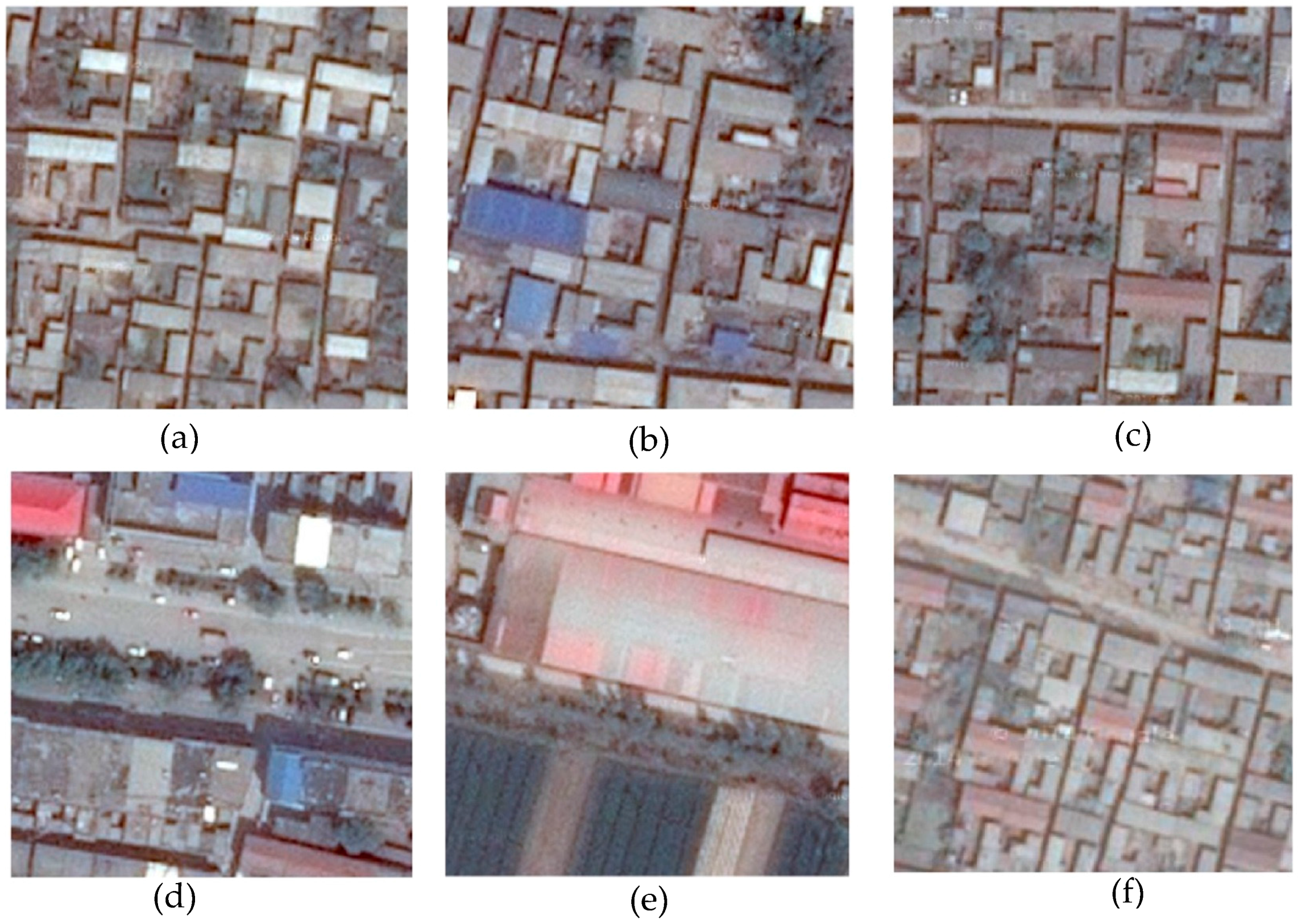
However, dihedral angle scattering not only relates to building density, but also relates to the spatial pattern of buildings because different areas with same density can display disparate intensity on account of their different distributions, sizes, and surroundings. As a result, backscatter intensity within a region can be influenced by both building density and spatial pattern. To illustrate this, six samples with similar densities (42.02%–44.71%) were selected and are shown in Figure 4. From data displays in

Table 2. Landscape metrics and intensity of samples with similar density.

Samples	Building Density (%)	Intensity(dB)	Fractal Dimension	Lacunarity
a	42.43	−15.81	2.4638	1.1056
b	42.22	−13.33	2.5566	1.1209
c	44.38	−15.33	2.6199	1.1536
d	42.02	−9.86	2.4378	1.1441
e	43.28	−16.91	2.1137	1.4574
f	44.71	−16.24	2.4821	1.1578

, it is obvious that intensities of those areas vary significantly due to buildings’ position, size, and existence of other object (e.g., a road or a lawn). Figure 4a,d shows two areas with almost totally same density (i.e., 42.43% and 42.02%) but disparate spatial features, which result in the fluctuant intensities (i.e., −15.81 and −9.86). When there is a lawn, as shown in Figure 4e, the intensity suddenly decreases to −16.91. Even the change of building size, as shown in Figure 4b,c, can cause fluctuation in intensities. These diverse intensities indicate that spatial pattern indeed plays an important role.

Therefore, backscatter intensity can highlight built-up areas and restrain some confusing areas (e.g., bare soil and other impervious surface). However, it does not strictly and precisely reflect the region’s building density. With the hope to solve this, a new index—amended backscatter intensity—is introduced. To achieve this, fractal dimension and lacunarity, which are also listed in Table 2, are used to depict the information of spatial pattern. Given that the 8 m-resolution GF-1 PMS image presents relatively clear spatial information and the calculation is time-efficient, GF-1 images will be the provider of those two indicators. The expectation for this index is to eliminate the effect of spatial pattern and make its value directly reflect the level of building density.

3.2.1. Fractal Dimension and Lacunarity

Fractal geometry was introduced and popularized by Mandelbrot as a means of describing highly complex forms characteristic of natural phenomena such as coastlines and landscapes [36] and has been widely applied to segmentation, classification, and characterization of the overall spatial complexity of remotely sensed images. Myint [37] employed it to classify urban land use types in Norman, Oklahoma, USA, and Jong [38] classified vegetation types in the Mediterranean.

Remotely sensed imagery can be viewed as fluctuating surfaces whose elevations correspond to the digital number values. In this sense, its fractal dimension ranges from two to three. Different landscapes have distinct spatial complexities, which leads to varying fractal dimensions. According to Qiu [39] and Lam [40], the most complex areas (i.e., urban areas) have the highest fractal dimension, while less complex rural settlements and farmland have lower fractal dimension. Similarly, within urban areas, regions with different building densities (e.g., residential areas, block junctions, industrial areas, and non-built-up areas) display extremely varying spatial complexity. Residential areas have many buildings, crisscrossing roads, and other types of objects. As such, they have the highest complexity and fractal dimension. Buildings in junction areas share the same features as residential areas, but the presence of a wide and homogeneous road lowers the complexity. Industrial areas are often occupied by large buildings with regular shapes and homogeneous backscatter intensity, and non-built-up areas such as farmland or natural landscapes are characterized as self-similar. Theoretically, the fractal dimension continuously decreases from residential to non-built-up areas.

The fractal dimension of a strictly self-similar object can be derived mathematically [41]:

$$D=\frac{\log (N_r)}{\log (1/r)}$$

(8)

where Nr represents the number of smaller copies of the object obtained by scaling its unit of measurement down by a ratio of r [36]. For non-self-similar objects, fractal dimension cannot be directly derived from this equation as a change in r will alter D; therefore, empirical estimation should be employed for such objects. Many algorithms have been proposed for calculating the fractal dimension of non-self-similar objects; here, we will employ improved triangular prism method developed by Sun [42].

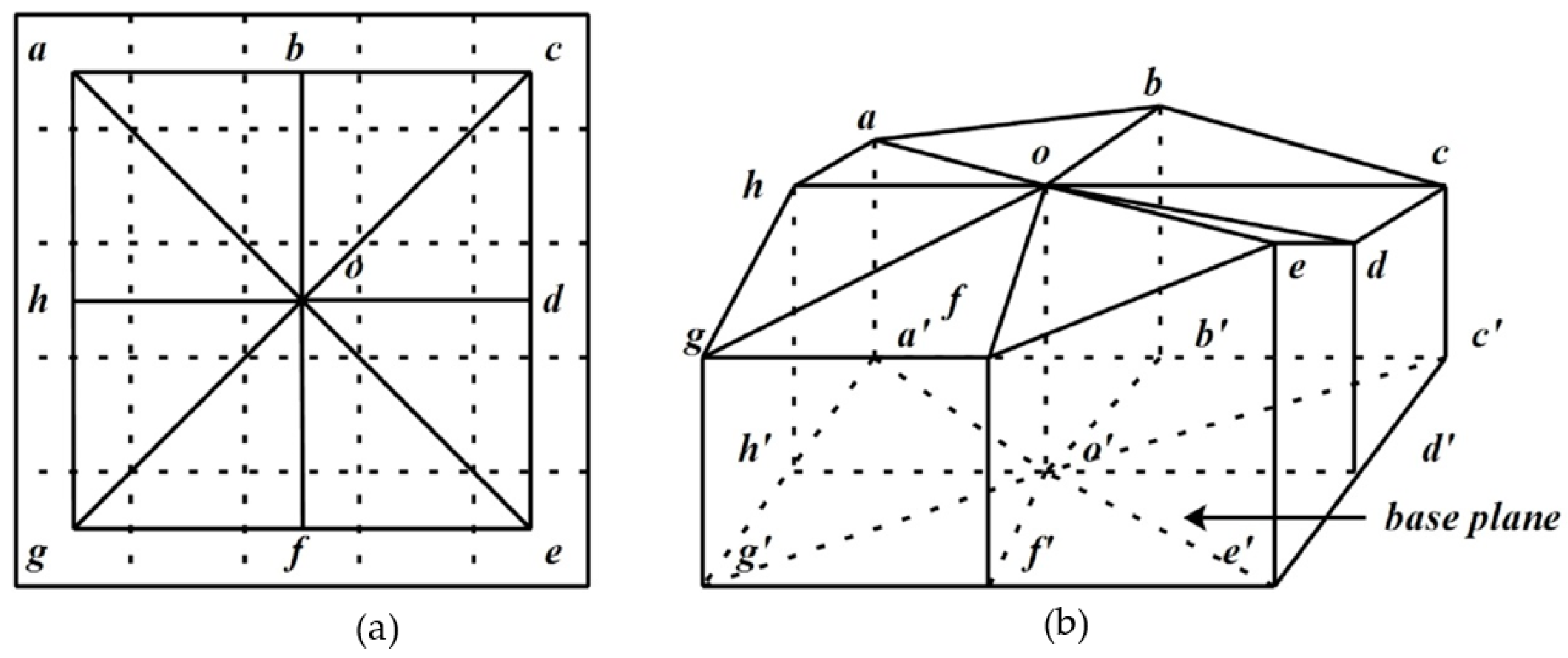
As illustrated by Figure 5, this method uses eight pixels on the edges of a square to represent the surface. According to Sun, four steps are implemented to obtain the fractal dimension.

Step 1: Calculate base distances. There are three different kinds of base distances. The first is the base distance between the central pixel and each of the corner pixels (e.g., $o{a}^{\prime },o{c}^{\prime },o{e}^{\prime },o{g}^{\prime }$ in Figure 5) and they are all equal to $\delta \times \sqrt{2}/2$, where $\delta$ is the side length of the base plain called step size. The second base distance is the one between the central pixel and middle pixel (e.g., $o{b}^{\prime },o{d}^{\prime },o{f}^{\prime },o{h}^{\prime }$ in Figure 6), which has the value of $0.5\delta$. The last one is the base distance between two neighboring edge pixels (e.g., $a{b}^{\prime },b{c}^{\prime },c{b}^{\prime },d{e}^{\prime }$ in Figure 6), which also has the value of $0.5\delta$.

Step 2: Calculate lengths of sides of triangles. Based distances together with the DN values of the central pixel, the corner pixels and the middle pixels are used to solve the lengths by the Pythagorean Theorem.

Step 3: Calculate of the top surface area. The top surface area of each prism then can be computed using Heron’s formula.

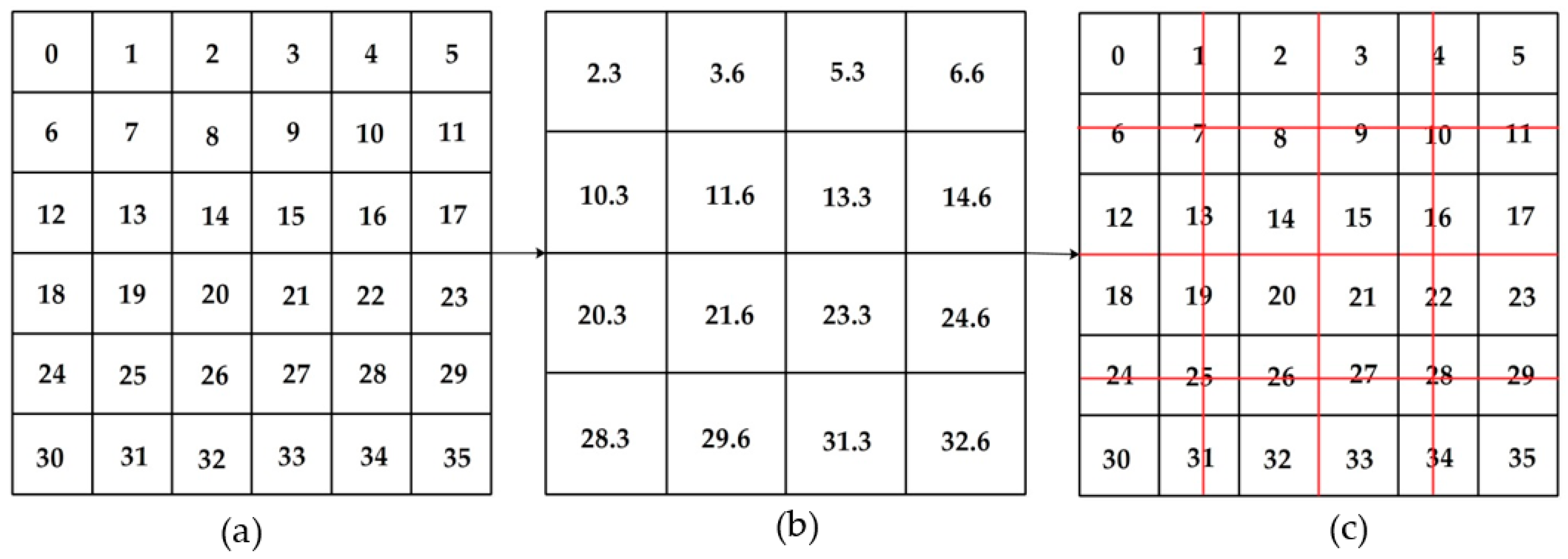
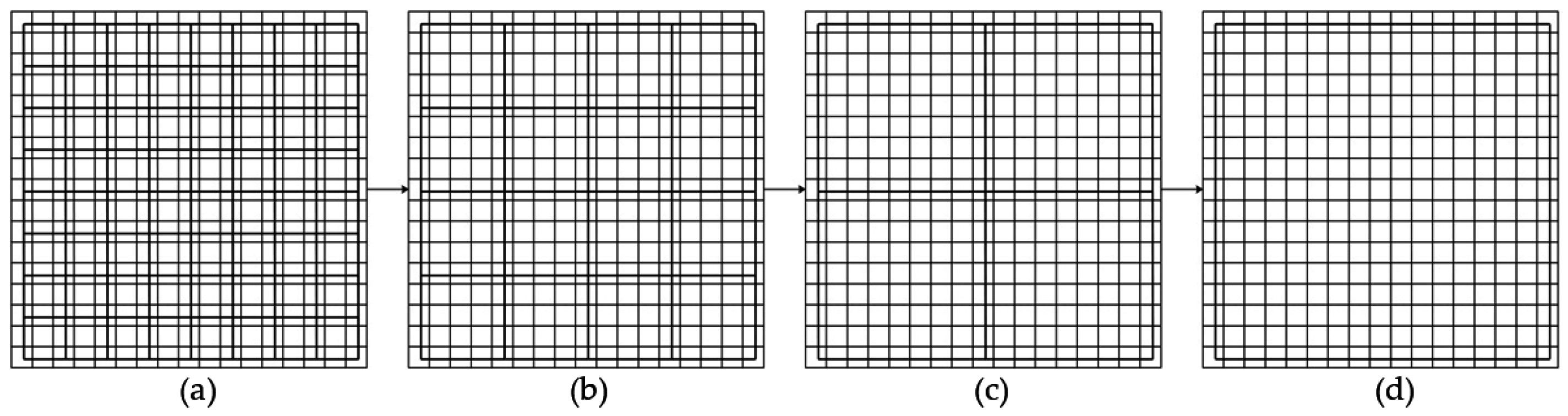
Step 4: Compute the fractal dimension value. The total area of the top surface can be calculated repeatedly for increasing step sizes by iterating Steps 1 to 3. As the size of the window used to cover the surface increases, more details in the top surface get lost and, as a result, the estimated total area of the top surface decreases (Figure 6). Once the total areas of the top surface are calculated for a certain number of step sizes, plot log (total top surface area) against log (step size) fit a least-squares regression line through the data points. The fractal dimension of the surface then is computed as $2-b$, where b is the slope of the log-log regression line.

The concept of lacunarity was originally proposed by Mandlebrot [41] to distinguish objects sharing the same fractal dimension but having differing appearance [43]. Lacunarity represents the distribution of gap size: low lacunarity geometric objects are homogeneous because all gap sizes are the same, while high lacunarity objects are heterogeneous [44].

Regions with different building density also show completely different lacunarity features owing to the discrepancies in building structures and surrounding objects. Buildings in residential areas are distributed regularly, homogeneously and at a small-scale, and are therefore less aggregated. Junction areas are more aggregated than residential areas owing to the presence of a middle-scale road. As industrial buildings are characterized as large scale because of their specific utility, they are the most aggregated.

Several algorithms have been proposed to calculate lacunarity, including Voss’s box counting algorithm [45], Dong’s differential box counting algorithm [46], Gan’s relative differential box counting algorithm [47], and Backes’ improved differential box counting algorithm [48]. Here, we chose relative differential box counting algorithm to calculate lacunarity.

The calculation is based on the equation:

$$\mathrm{\Lambda }(r)=\frac{{\displaystyle \sum _M{M}^2}Q(M,r)}{{\left[{\displaystyle \sum _{M}M}Q(M,r)\right]}^2}$$

(9)

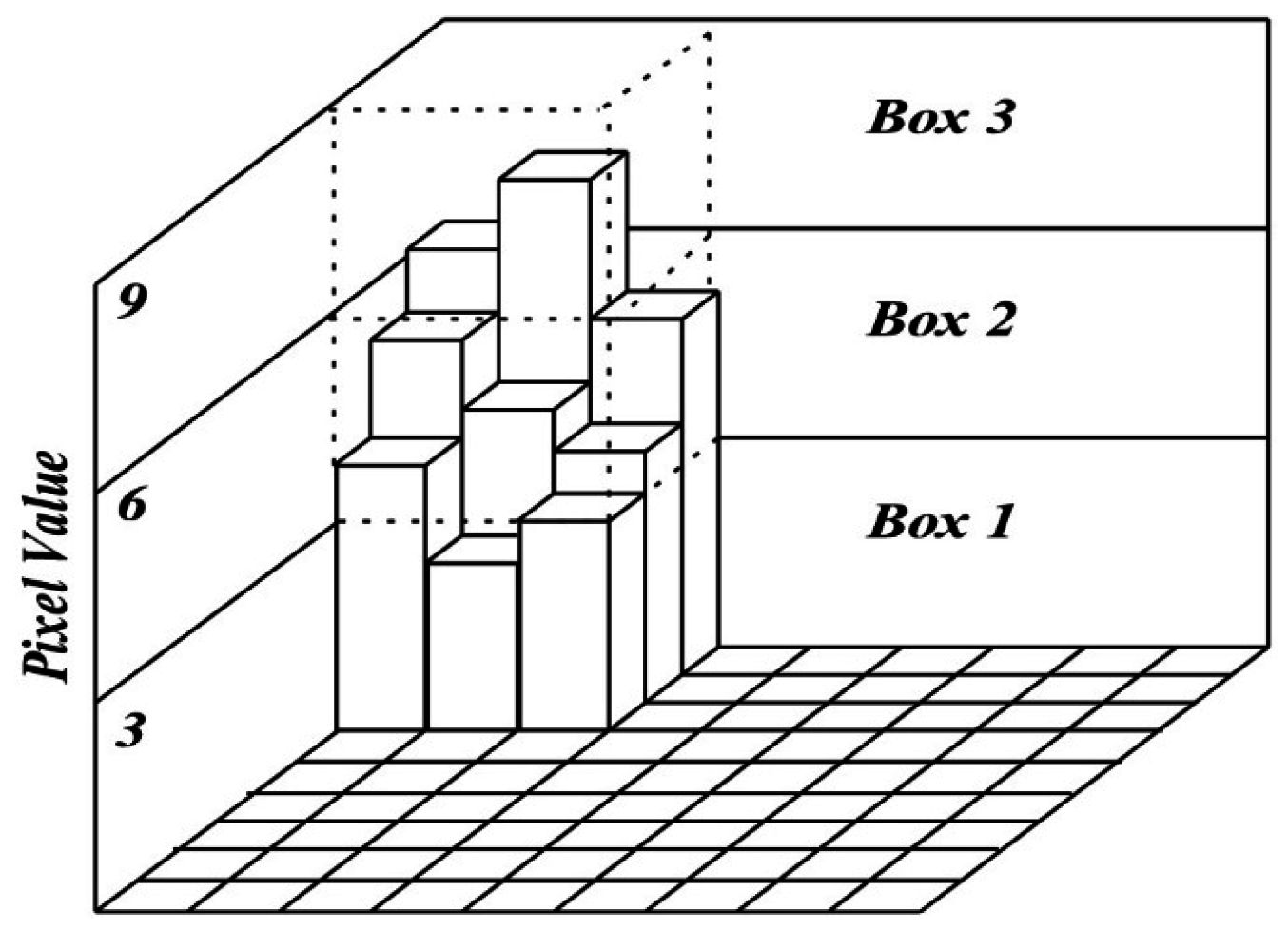
As shown in Figure 7, a cubic of size $r\times r\times r$ is placed over the upper left corner of an image window of size $w\times w$, which is an odd number, and $r\le w$. Depending on the pixel values in the $r\times r$ gliding-box, a column with more than one cube may be needed to cover the image intensity surface. Assign numbers 1, 2, and 3 to the cubic boxes from bottom to top. For each $r\times r$ gliding-box, let the minimum and maximum pixel values in the gliding-box fall in box number u and v, respectively. Then the relative height of the column is:

$$n_r(i,j)=v-u-1$$

(10)

where i and j are image coordinates. When the $r\times r$ gliding-box moves throughout the $w\times w$ image window, we have:

$$M_r={\displaystyle \sum _{i,j}ceil\left[k{n}_r(i,j)/h\right]}$$

(11)

where k is expressed as $k=w/g$, and g is the maximum pixel value within the $w\times w$ window. The M in the equation is replaced by M_r. Define $n(M,r)$ to be the number of gliding boxes with size r and mass M_r, and then $Q(M,r)$ can be defined as

$$Q(M,r)=\frac{n(M,r)}{{(w-r+1)}^2}$$

(12)

3.2.2. Deviation Degree

Before calculating amended backscatter intensity, an important concept called deviation degree (DD) should be introduced. According to previous studies on lacunarity and fractal dimension, we know that lacunarity ranges from 1 to infinity and fractal dimension ranges from 2 to 3 when applied to satellite images. Generally, areas with homogeneous surface (e.g., a water body or farmland) can be viewed as having only one significant gap. Therefore, they have infinite lacunarities. Because building areas are dotted with many gaps, their lacunarities range from 1 to 2 in most cases. Areas with high complexity, as discussed in Section 3.2.1, have a high fractal dimension; thus, DD is defined as

$$DD=\left[\left(LCU-1\right)+\left(3-FD\right)\right]/2$$

(13)

where LCU represents lacunarity and FD represents fractal dimension. Considering that most lacunarities are lower than 2 with only 3% out of this range, lacunarities higher than this value were set to 2.

As previously discussed, the value of $(3-FD)$ only represents the degree of being away from highly complex and even two regions sharing same value can show totally different distribution pattern. The addition of $(LCU-1)$ complements this by representing the degree of being away from homogeneously distributed. Therefore, DD is a comprehensive effort about complexity and distribution. The coefficient $1/2$ was used for normalization. It is obvious that the more an area deviates from being homogenously distributed and highly complex, the higher its DD becomes.

3.2.3. Calculation of Amended Backscatter Intensity

With DD, the new feature—amended backscatter intensity (ABI)—could be generated by following equation.

$$ABI=BI\times (1\pm DD)$$

(14)

The key point of this Equation (14) is to determine whether the coefficient of DD should be 1, −1, or 0, i.e., to determine whether ABI is higher than BI or lower. Things differ in different areas. In industrial areas, building densities are relatively high, usually up to 50% or above. However, their BI are not correspondingly high, thus the ABI should be increased. In non-built-up areas, of course with building density of 0%, although most of them have low BI, they cannot be clearly distinguished from low density areas. Therefore, their ABI should be decreased. From this point, a classification is required to determine the coefficient for each urban land use class before the calculation of ABI. Similarly, CART algorithm will be employed to perform the classification.

3.3. Accuracy Assessment

The quality of the constructed regression tree was measured using root-mean-square error (RMSE) and determination coefficient (R²). Besides, an F-test might be useful to examine the significance of regression coefficient although it is not directly related to the precision.

Note that an n-fold cross-validation is available in Cubist. Using this option, the training dataset can be divided into n blocks of roughly equal size. For each block in turn, a model is built from the data in the remaining blocks and validated using the holdout block. The final accuracy of the model is estimated by averaging model results from all n-fold tests [49].

4. Result

4.1. Distribution of Deviation Degree

Figure 8 shows 12 sample areas with various distribution and complexity. From

Table 3. Landscape metrics and deviation degree of different building areas with different distribution patterns.

Samples	Fractal Dimension	Lacunarity	Deviation Degree
a	2.4541	1.1461	0.3460
b	2.5445	1.0853	0.2704
c	2.2360	1.3400	0.5520
d	2.4881	1.3036	0.4078
e	2.1683	1.3282	0.5799
f	2.2017	1.2906	0.5445
g	2.4811	1.1354	0.3272
h	2.1176	2.0000	0.9412
i	2.0015	1.5323	0.7654
j	2.4283	1.1529	0.3623
k	2.5583	1.1158	0.2788
l	2.5565	1.1898	0.3166

, we can see that areas with relatively homogeneous distribution and high complexity (e.g., residential areas in Figure 8b,g,j,k have correspondingly lower DD while a flat, long road, a huge workshop, or other large, homogeneous non-building objects can cause an enhancement in DD).

Figure 9 shows the distribution of DD. In Figure 9a, water has highest DD and so do the two crisscross long roads. Farmland has relatively lower DD than water and road and most part of the city and town are unremarkable expect for some industrial regions and suburbs which have irregular building distribution and homogeneous land cover. In Figure 9b, water shows similarly high DD and the airport at the upper right corner has high DD as well. Most built-up areas in the downtown have lower values than those of non-built-up areas.

4.2. Establishment of Decision Rules

Based on spatial patterns of 200 training/validation samples of Jizhou, we classified them into six types: non-built-up area, water, low density area, middle density area, high density area, and very high density area. Non-built-up areas include farmland and manmade bare surface. Low density areas can usually be regarded as suburbs or peri-urban areas and existence of large area farmlands and undeveloped lands lead to low building densities, which are lower than 20 percent at most of the time. Middle density areas usually locate inside the city or town but are close to a road, a street, a park or other public facilities and are with building densities between 20 and 30 percent. High density areas are often with a building density ranging from 30 to 50 percent and are predominated by residential and commercial areas. Very high density areas have large buildings and can easily reach densities of 50–70 percent, and even 100 percent.

Things are different in Beijing due to more diverse building types and more complex urban planning strategies. Therefore, a different classification scheme was used: non-built-up area, water, workshop-like function area, high density level community, low density level community, industrial area, and non-residential built-up area. Workshop-like function areas look like workshop but mainly used as market or residential area and often located in peri-urban areas with low floor and medium scale size. High density level communities are traditional communities and their buildings are usually lower than 6–8 floors and often distributed close to each other. Low density level communities are communities in modern style and their buildings are lift apartment with more than 20 floors. Greening rate is often required in those communities, thus buildings are widely separated by green land. Non-residential built-up areas are used for business or commerce with different looks from residential areas.

In Jizhou, non-built-up areas such as farmland are usually homogeneous and less complex with high DD. However, its BI is sometimes overlapped and confused with built-up area, so the coefficient is 1 in order to distinguish non-built-up area from built-up area. Water areas basically share the same feature with non-built-up areas, but have lower BI. Therefore, to keep their ABI in line with those of non-built-up areas, the coefficient is 0. High density areas and very high density areas are similar in BI, but the DD of very high density area is higher than that of high density area. Thus, when the coefficient is set to −1 for both, very high density areas will have higher ABI than high density area. For middle density areas, they have higher BI than low density areas but a similar DD. To completely differentiate these two and avoid the overlap between middle density areas and high density areas, the coefficients of these two are both set to 1. Therefore, the ABI of these two will be lower than those of high density and very high density areas but higher than non-built-up areas and water areas. Besides, the ABI of middle density areas are still higher than that of low density areas.

In Beijing, non-built-up areas and water areas are similarly treated as in Jizhou. For high and low density level communities, if the coefficients are both set to 1, their ABI will overlap with those of non-built-up and water areas, while, if are both set to −1, it is still difficult to distinguish them due to their similar BI and DD. Therefore, the coefficient of low building density level communities is 0 while that of high building density level communities is −1. If the coefficient for non-residential built-up areas is set to 1 or 0, their ABIs will be confused with those of non-built-up areas and low density level communities, respectively; thus, the coefficient for it is −1. Based on this, coefficients for workshop-like function areas and industrial areas are both −1 and their ABIs will be higher than that of non-residential built-up areas but similar to each other.

Through this determination scheme, values of ABI basically correspond to building densities.

Characteristics of each class are listed in

Table 4. Features and coefficient for each class.

Jizhou			Beijing
Class	Characteristics	Coefficient	Class	Characteristic	Coefficient
Non-built-up Area (0%)	Backscatter intensity $\le -20$;	1	Non-built-up Area (0%)	Backscatter intensity $\le -16$;	1
	Fractal dimension $\le 2.3$;			Fractal dimension $\le 2.3$;
	Lacunarity $\ge 1.25$;			Lacunarity $\ge 1.15$;
	Deviation degree $\ge 0.5$			Deviation degree $\ge 0.45$
Water (0%)	Backscatter intensity $\le -30$;	0	Water (0%)	Backscatter intensity $\le -22$;	0
	Fractal dimension $\le 2.1$;			Fractal dimension $\le 2.1$;
	Lacunarity $\ge 1.25$;			Lacunarity $\ge 1.3$;
	Deviation degree $\ge 0.5$			Deviation degree $\ge 0.5$
Low density area (14.29%)	Backscatter intensity $\in (-19,-16)$;	1	Workshop-like function area (60.40%)	Backscatter intensity $\in (-16,-11)$;	−1
	Fractal dimension $\le 2.3$;			Fractal dimension $\in (2.2,2.4)$;
	Lacunarity $\ge 1.15$;			Lacunarity $\in (1.1,1.3)$;
	Deviation degree $\ge 0.4$			Deviation degree $\in (0.5,0.7)$
Middle density area (29.88%)	Backscatter intensity $\ge -14$;	1	High density level community (27.53%)	Backscatter intensity $\in (-16,-11)$;	−1
	Fractal dimension $\in (2.2,2.5)$;			Fractal dimension $\in (2.1,2.4)$;
	Lacunarity $\in (1.1,1.3)$;			Lacunarity $\in (1.1,1.4)$;
	Deviation degree $\in (0.3,0.5)$			Deviation degree $\in (0.4,0.5)$
High density area (36.26%)	Backscatter intensity $\in (-16,-12)$;	−1	Low density level community (10.12%)	Backscatter intensity $\in (-16,-10)$;	0
	Fractal dimension $\ge 2.5$;			Fractal dimension $\in (2.1,2.4)$;
	Lacunarity $\le 1.15$;			Lacunarity $\in (1.1,1.4)$;
	Deviation degree $\le 0.4$			Deviation degree $\in (0.3,0.65)$
Very high density area (50.34%)	Backscatter intensity $\in (-16,-12)$;	−1	Industrial area (64.05%)	Backscatter intensity $\in (-19,-13)$;	−1
	Fractal dimension $\in (2.3,2.5)$;			Fractal dimension $\in (2.1,2.35)$;
	Lacunarity $\ge 1.2$;			Lacunarity $\in (1.2,1.55)$;
	Deviation degree $\ge 0.4$			Deviation degree $\in (0.4,0.7)$
\	\	\	Non-residential built-up area (17.96%)	Backscatter intensity $\in (-17,-12)$;	−1
				Fractal dimension $\in (2.1,2.4)$;
				Lacunarity $\in (1.15,1.3)$;
				Deviation degree $\in (0.3,0.5)$

.

The classification accuracy was assessed by 200 testing samples (100 for Jizhou and 100 for Beijing) and is displayed in

Table 5. Accuracy analysis of classification results.

Jizhou			Beijing
Class	Produce Accuracy (%)	User Accuracy (%)	Class	Produce Accuracy (%)	User Accuracy (%)
Non-built-up area	81.25	81.25	Non-built-up area	78.57	86.42
Water	94.12	88.89	Water	85.71	92.31
Low density area	70.59	66.67	Workshop-like function area	60.00	56.25
Middle density area	50.00	47.06	High density level community	64.28	90.00
High density area	58.82	71.43	Low density level community	53.33	44.44
Very high density area	70.59	70.59	Industrial area	78.57	64.71
\	\		Non-residential built-up Area	50.00	53.85
Overall accuracy	71.00		Overall accuracy	67.00

.

The result demonstrated that the classification performed better when ground objects are simple and homogeneous (e.g., water, non-built-up area, and high density industrial area) but were weak in classifying classes with complex structure and object type like middle density area and low density area.

Note that the classification process was done by programming with Python using CART algorithm due to the inability for Cubist to deal with discrete variables.

4.3. Distribution of Amended Backscatter Intensity

As displayed in Figure 10, the calculation of fractal dimension and lacunarity employed three optical bands of GF-1 PMS images and the final results are average values of them. During this process, we chose a 13 × 13 window ($13\times 8 m=104 m\approx 100 m$); box sizes 3, 5, 7 and 9 for lacunarity; and step sizes 2, 4 and 12 for fractal dimension.

The distribution of ABI is displayed in Figure 11. We can see that some bright farmlands, roads, and most parts of non-built-up areas in Figure 11a are effectively restrained. Moreover, some empty regions in urban and rural areas are more obvious in Figure 11b. Compared to Figure 11c, built-up areas with almost all kinds of building types in Figure 11d are enhanced, especially the originally weakly-scattered airport at the upper right corner. The difference between non-built-up areas and built-up areas also becomes more noticeable.

4.4. Comparison between Different Models

Models with different input features are established by CART algorithm and their brief descriptions are shown in

Table 6. Models with different input features.

Models	Input Features
a	B1–4
b	NDVI, NDWI, RBI
c	BI
d	ABI
e	B1–4, NDVI, NDWI, RBI
f	B1–4, BI
g	B1–4, ABI
h	B1–4, NDVI, NDWI, RBI, BI
i	B1–4, NDVI, NDWI, RBI, ABI

. To guarantee the accuracy, a 10-fold cross validation was used when constructing the regression tree and the average of 10 models was used as the final result.

Overall, building density distributions from nine models were mapped and displayed in Figure 12 and Figure 13 for Jizhou and Beijing, respectively. Those nine models can be divided into two groups.

The first group includes models a, b, c and d, which are shown as Figure 12a–d and Figure 13a–d, respectively. Building density estimation of those models basically follows the characteristics of the input feature itself. For example, in Figure 12 (Jizhou), model a has a lot of overestimation in bare soil and other impervious surface because of the spectral similarity; model b only improves the estimation in water area but lacks accuracy in other regions; and model c and model d are similar with the distribution pattern of BI and ABI on the whole but model d shows a better ability in reducing error in farmland and roads. In general, model d shows remarkable improvement in prediction compared with the other three. In Figure 13 (Beijing), model a still cannot precisely distinguish between most of the built-up areas and non-built-up areas and shows an overall underestimation; model b can hardly perform a correctly prediction; and both model d and model c display an overall underestimation similar to model a.

The second group includes models using a combination of several features. All of them improve more or less in contrast to models in the first group. For example, in Figure 12e, i.e., model e, although it still overestimated plenty of farmland, ameliorates the water in model a and the road in model b; model f and model h have less overestimation in farmland and have diverse density distribution in urban area; and model g and model i seem to have the best capacity in restraining the overestimation and have variant density patterns in urban area. In Figure 13, model e modestly fixes the underestimation problem but still shows mixture between built-up and non-built-up areas; and models f, g, h, and i are closer to reality but differ in the density level in some places.

Statistically, the root-mean-square error (RMSE) and determination coefficient (R²) were calculated. Meanwhile, an F-test was done to examine the reliability of each model. The results are displayed in

Table 7. Accuracy assessment for different models for Jizhou.

Model	Jizhou			Beijing
	RMSE	R2	p	RMSE	R2	p
a	15.45	0.35	0.01/0.005/0.025	21.78	0.26	0.025/0.01
b	16.57	0.43	0.005	24.23	0.19	0.025
c	12.71	0.48	0.025	21.56	0.24	0.005
d	11.53	0.58	0.005	20.34	0.30	0.01/0.005
e	10.28	0.63	0.005	20.34	0.36	0.05/0.025
f	10.33	0.60	0.005/0.025	18.29	0.49	0.005/0.01/0.005
g	9.54	0.77	0.005	16.91	0.54	0.005/0.005
h	10.73	0.60	0.005/0.01/0.005	17.58	0.52	0.025/0.005/0.025
i	8.93	0.80	0.005	16.21	0.64	0.05/0.025

Note: Each model may have one or more p value(s) since the CART algorithm can generate one or more equations under different decision rules for each model.

.

Model b, which uses NDVI, NDWI and RBI, has the weakest prediction ability, while model a does better than model b. Their combination (i.e., model e) improves the accuracy by 5.1696 and 6.284 in RMSE, and 0.2736 and 0.1973 in R² for Jizhou and 1.4313 and 3.8851 in RMSE, and 0.0952 and 0.1681 in R² for Beijing, respectively. Models using BI have similarly low accuracy as the aforementioned models. In those four models, SAR parameters do not integrate into optical parameters and the most precise model has RMSE of 10.28 and R² of 0.63 for Jizhou and RMSE of 20.34 and R² of 0.36 for Beijing.

Models d, f, g, h and i symbolize the synergistic use of two data sources and expectedly enhance the accuracy. Among them, model i has the highest R² and lowest RMSE, which are 0.80 and 8.93, and 16.21 and 0.64 for Jizhou and Beijing, respectively. Model d can improve the result to some degree, but, as we analyzed previously, it lacks density diversity in urban area and the addition of optical features seems to make up for this problem. Although the other three models are less accurate than model i, they make a relatively precise prediction as well.

5. Discussion

Building densities are likely to be overestimated in areas containing other impervious surfaces and bare soil because buildings share the similar spectral signatures with those elements when using optical imagery alone. Unlike optical images that represent the spectral reflectivity, SAR images are very sensitive to the surface roughness, shape, structure, and dielectric properties and can provide information complementary to optical data. In our study, we synergistically used GF-1 PMS and Radarsat-2 data for building density estimation and proposed a new feature being exempted from the influence caused by spatial pattern. The result shows that the combination of two data can indeed improve the problem of overestimation in non-built-up areas that share the same spectral signature with buildings and the addition of the new feature further enhance the accuracy. Besides, when compared with other research related to regression modeling, this result is better than that of the study in Munich, Germany using random forest algorithm, which has a RMSE of 10 and R² of 0.63 [35]. Although Zheng’s study [26] has a higher precision with RMSE of 2.16, it only tested 10 samples. Therefore, its result is not convincing. When it comes to the automatic building detection, Yu [20] reached an overall accuracy of 96%; Wu [21] decreased average absolute error to 6.6% after employing the threshold segmentation; Kajimoto [23] obtained correlations of 0.866, 0.852, 0.772, and 0.566 for 100 m, 200 m, 300 m and 500 m scale, respectively; and Susaki [24] extended Kajimoto’s way to multiple PolSAR images reaching a correlation of 0.820. Kajimoto and Susaki’s research employed moderate resolution imagery, which reduce the data size and processing time but at the cost of the accuracy decrease. Therefore, it seems that there is a tradeoff between resolution and accuracy when using automatic building detection. Compared to those results, the result of this study is less accurate than those using high-resolution imagery but more time-efficient and more accurate than those using similar time efficient moderate resolution imagery.

Two study areas (i.e., Jizhou and Beijing) have totally disparate urban morphology and building types and the images are acquired in different seasons. These factors can have an influence on optical spectral reflectance, BI and further the calculation of fractal dimension, lacunarity and ABI. The positive result demonstrated that the variances of these input features do not have a significant impact on the effectiveness of our method, which successfully proves the robustness and transferability of it. Another breakthrough lies in the proposed indices (i.e., DD and ABI). The former has the potential to delineate the spatial pattern of a region, which might be of great value in fine-scale urban classification. The latter is a good indicator of building density and can contribute to prospective research focusing on building density estimation.

Despite the improvement on accuracy, it seems to have better performance in Jizhou than in Beijing, both before and after combining multisource data. This might be caused by the fact that megacities like Beijing have a more complex urban landscape and morphology, which can have a remarkable influence on optical spectrum and SAR backscattering within a region.

Besides that, some other problems need to be stated and discussed:

• When generating ABI, we only cared about the influence caused by spatial pattern, but ignored height, building orientation, shadow and layover. To sum up, it is a 2D-based method without consideration of 3D information.
• The 8 m resolution GF-1 image is relatively coarse and may lose some detailed information when calculating fractal dimension and lacunarity.
• In determining the coefficient of DD, we have developed a series of decision rules to classify the image into some types. However, the selection of class varies from city to city and the coefficient determination need extensive analysis. Therefore, a unified classification scheme and an automatic method for determining coefficient are urgently needed.
• Testing samples were manually selected, and although randomness was emphasized during the selection, a small number of samples is insufficient for representing the entire region.
• The study area is a plain where the landscapes are relatively simple (e.g., the regularly-shaped, and equally-scaled farmland). However, when the method is extended to a hilly area, it may not be that precise since the natural landscapes will be more complex and their landscape metrics may be difficult to distinguish with building areas.
• The problem for seasonality persists. Although the result showed that the calculations of fractal dimension, lacunarity, and deviation degree are not affected, we cannot be certain whether the overall higher backscatter intensities are caused by seasonality or incidence angle or building types. Therefore how different seasons will affect the SAR backscattering pattern needs to be addressed in the future.

6. Conclusions

This study focused on large scale building density estimation by using integration of SAR and optical data and was successfully conducted in Jizhou and Beijing by applying the CART algorithm to the GF-1 PMS and the Radarsat-2 SAR data. In addition to B_1–4, NDVI, NDWI, RBI, and BI, a new index ABI was proposed as a potential feature to improve the accuracy. Before the integrated use of two data sources, model using B_1–4, NDVI, NDWI and RBI had the highest accuracy, i.e., the RMSE of 10.28 and R² of 0.63 for Jizhou and the RMSE of 20.34 and the R² of 0.36 for Beijing. Compared with this, the best model after combining two data, i.e., the model employing B_1–4, NDVI, NDWI, RBI, and ABI, reduces RMSEs to 8.93 and 16.21, and raises R²s to 0.80 and 0.64. Result of this study showed that the synergistic use of different sensors and satellites has the potential to improve the building density estimation performance, especially in separation of land uses that have spectral signatures similar to building areas, which has been a tough task when merely using optical data. It also showed that, although currently existing indices (i.e., B_1–4, NDVI, NDWI, RBI and BI) can represent the characteristics of built-up areas, new indices and features are still necessary. The newly proposed index (i.e., ABI) has shown its potential to enhance the accuracy of building density estimation and should be carefully considered in further studies.

Some problems still exist, as discussed previously, however, the results from this study show the potential for using combination of SAR and optical data in building density mapping. Future work relating to this methodology will address the above-mentioned five problems and will involve the development of an algorithm for calculating lacunarity and fractal dimension in order to determine accuracy when employing different algorithms. Determining the relationship between building density and human distribution is our final objective; to achieve this, other reference information such as building height and land cover might have to be used in conjunction with building density.