
A Generic Framework for Assessing the Performance Bounds of Image Feature Detectors †


Abstract
:
1. Introduction
2. Related Work
3. The Proposed Framework
- (a)
- The ability to determine the upper and lower performance bounds of a given detector under some specific type and amount of image transformation—an idea borrowed from electronic systems design practice.
- (b)
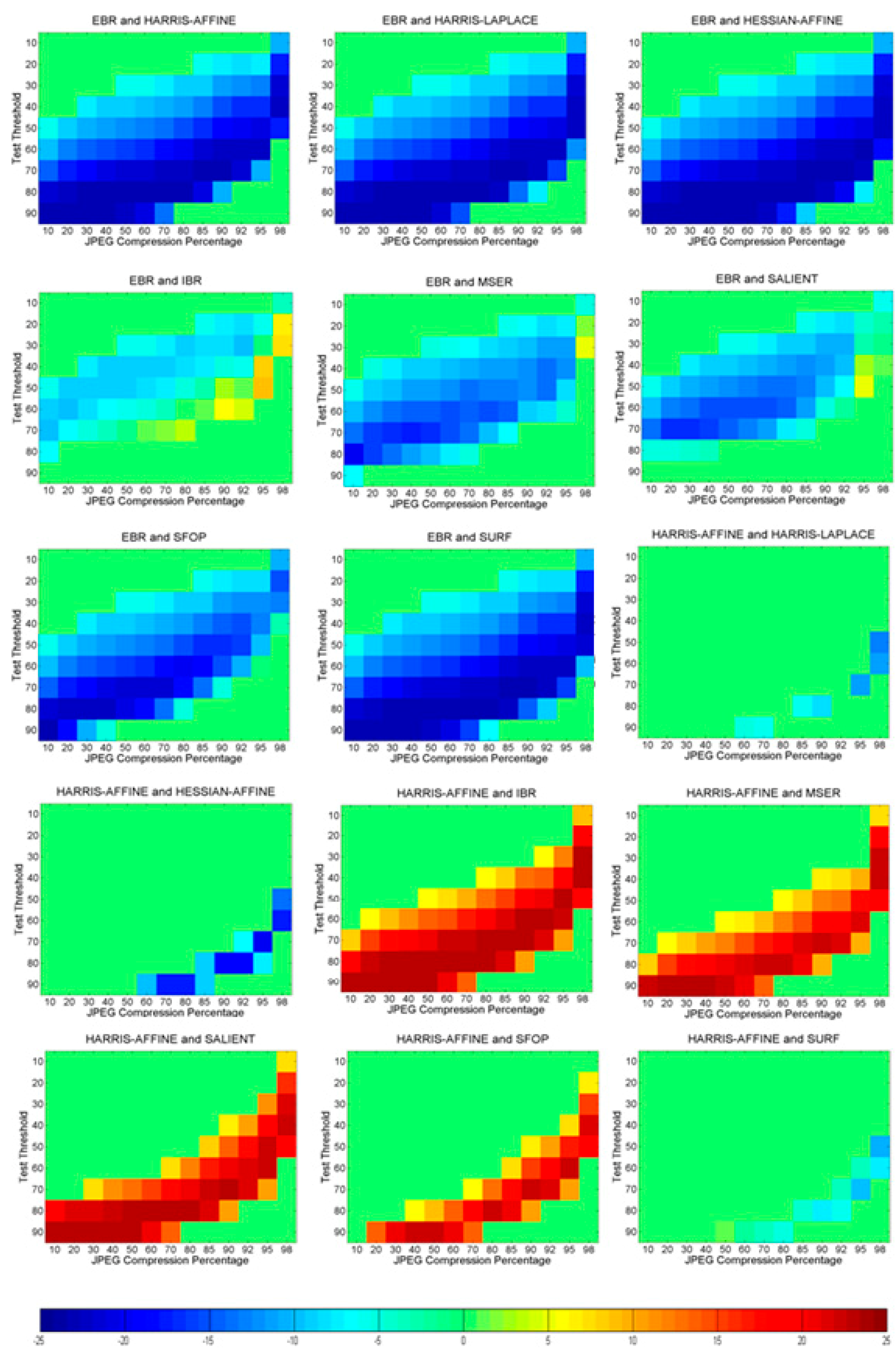
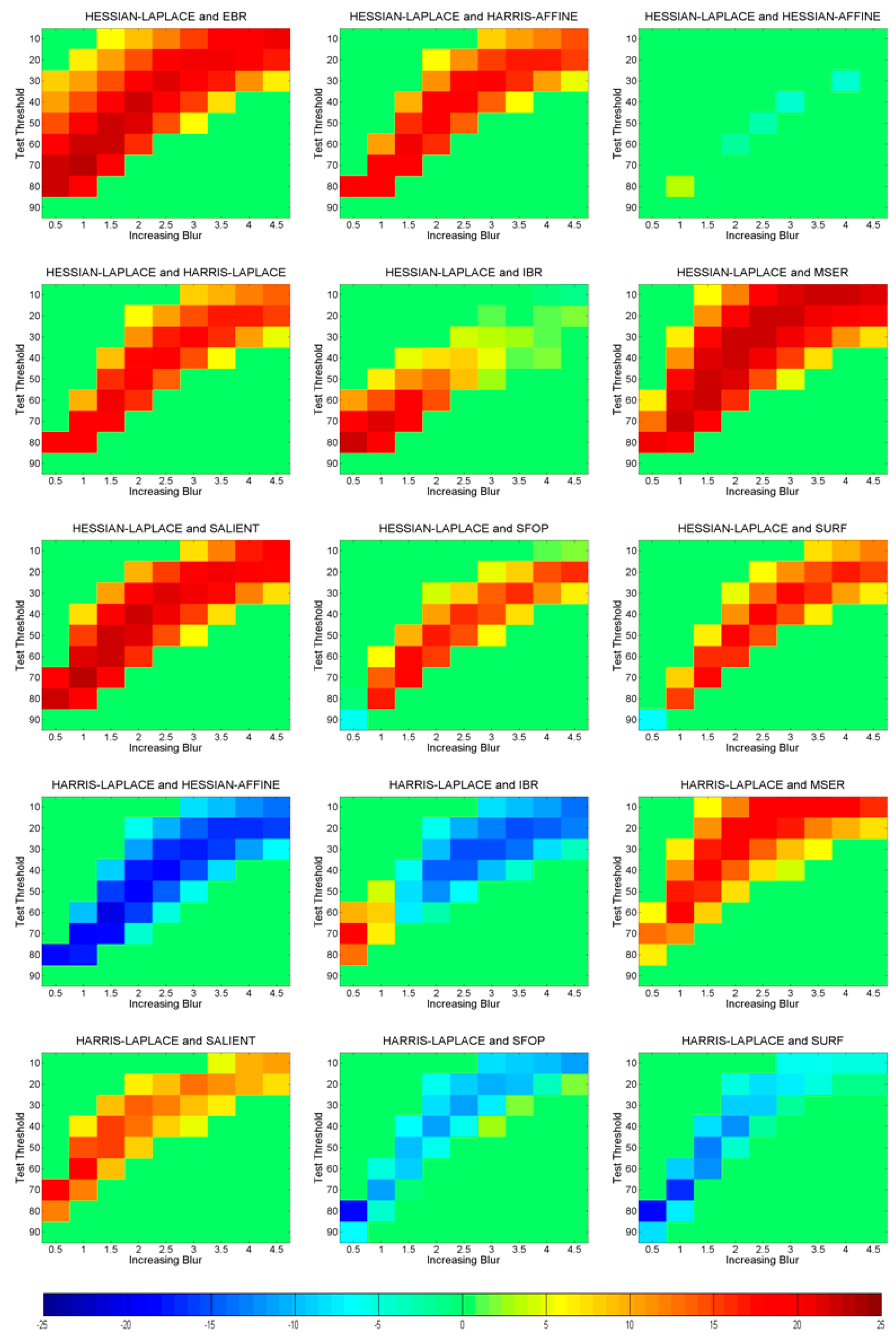
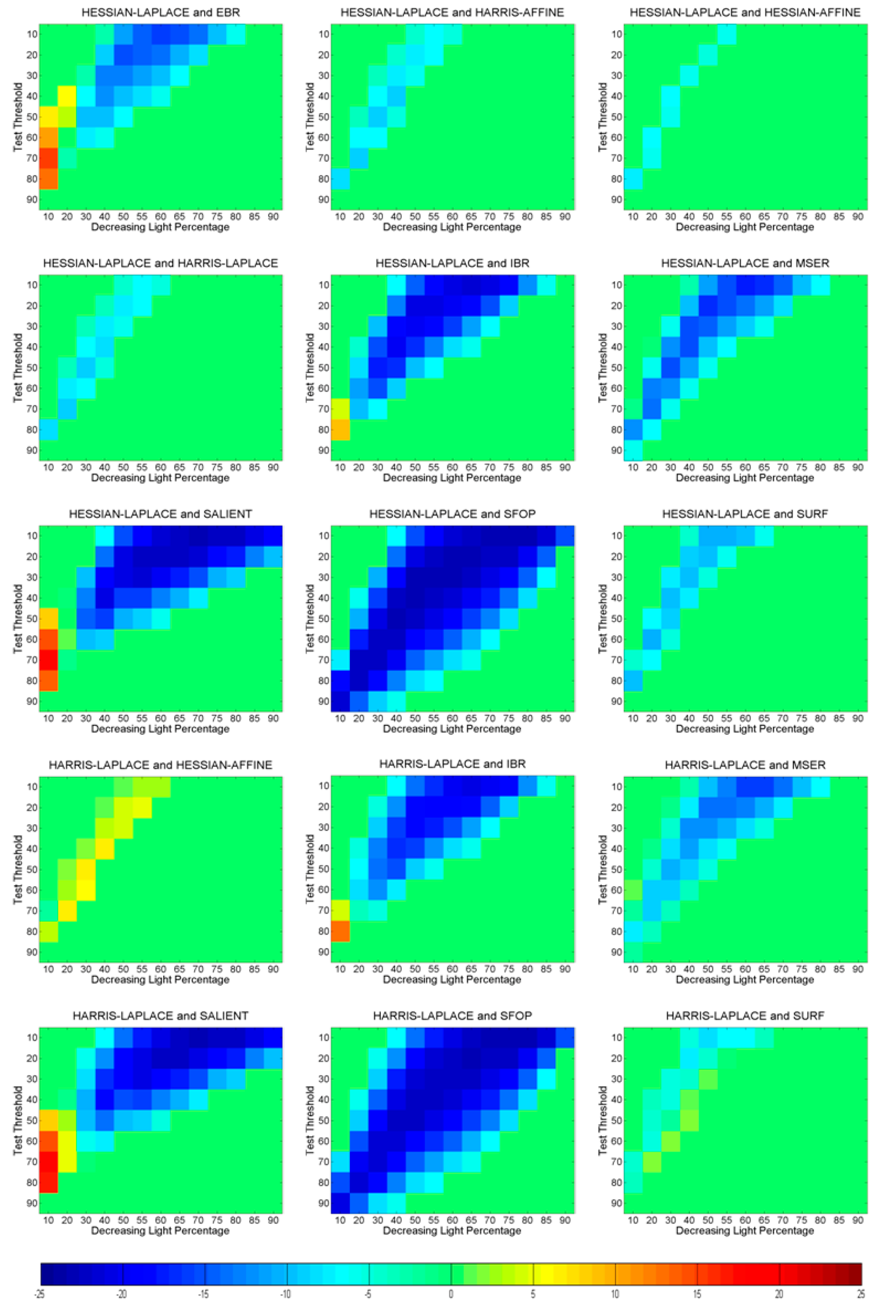
- The ability to identify statistically significant performance differences between a given detector and some other detector whose performance is considered a benchmark under specific type and amount of image transformation—a concept for taking into account the comment made by [4].
3.1. Phase 1: Identification of Operating and Guarantee Regions
- (a)
- The repeatability scores are computed using Equation (1) for all images in every individual dataset (of the large image database) by taking the first image in each dataset which contains no transformation, as the reference. Assuming that the amount of image transformation is varied in m discrete steps for every single dataset, n values of repeatability are obtained for each discrete step. Let A be the set of m discrete steps representing specific transformation amountsLet be the set of n repeatability values at any one specific step , where is an element of set AFor example, if the image database consists of 539 different datasets (the number which will be used in the next few sections), each consisting of a sequence of 14 images, the values of n and m will be 539 and 14 respectively. In other words, there will be 539 values of repeatability available for each step of image transformation amount.
- (b)
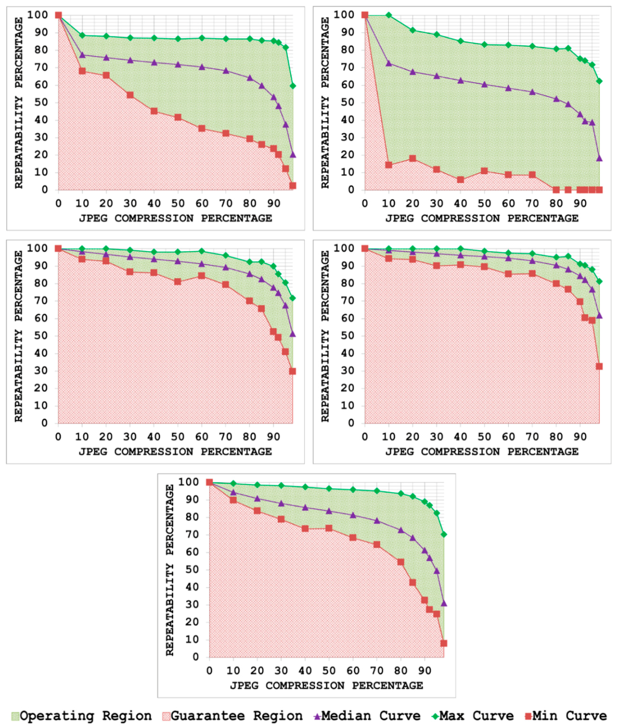
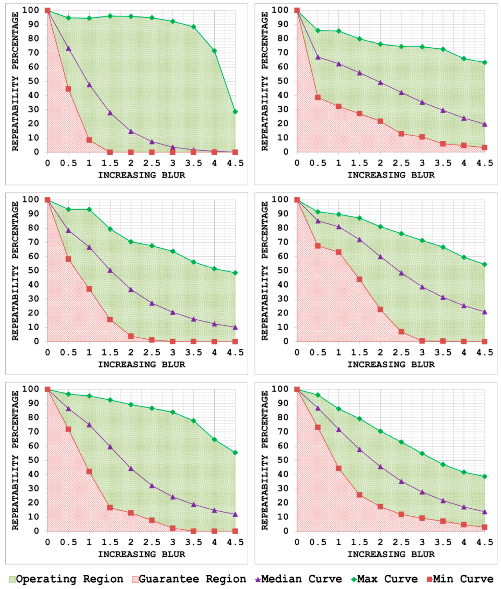
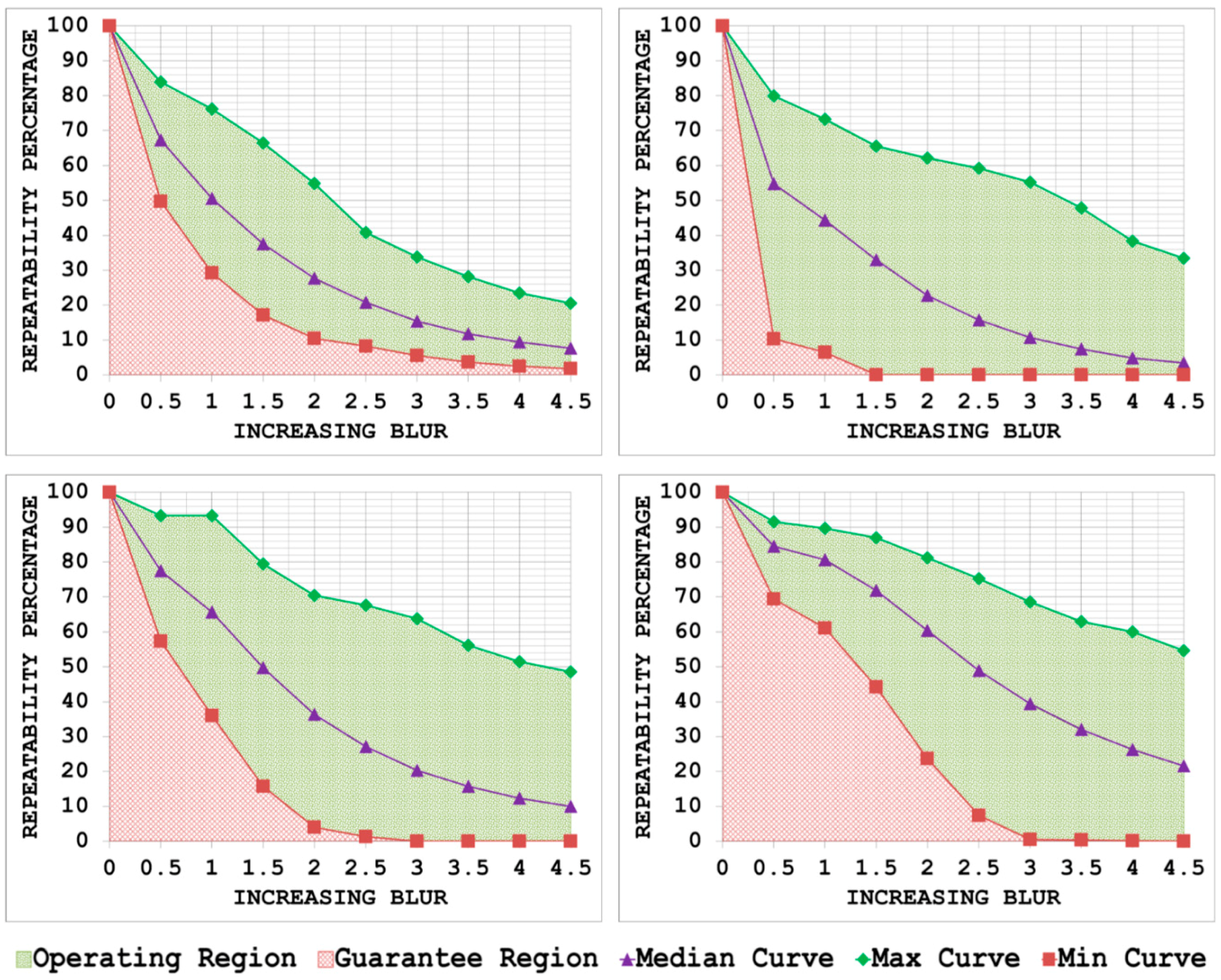
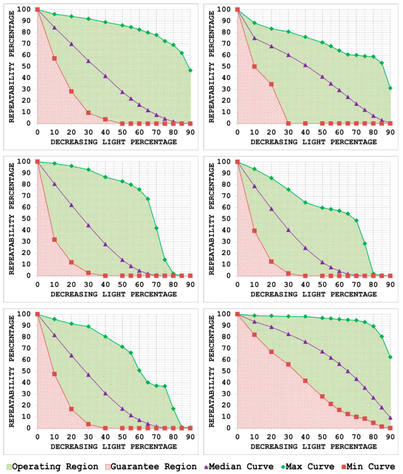
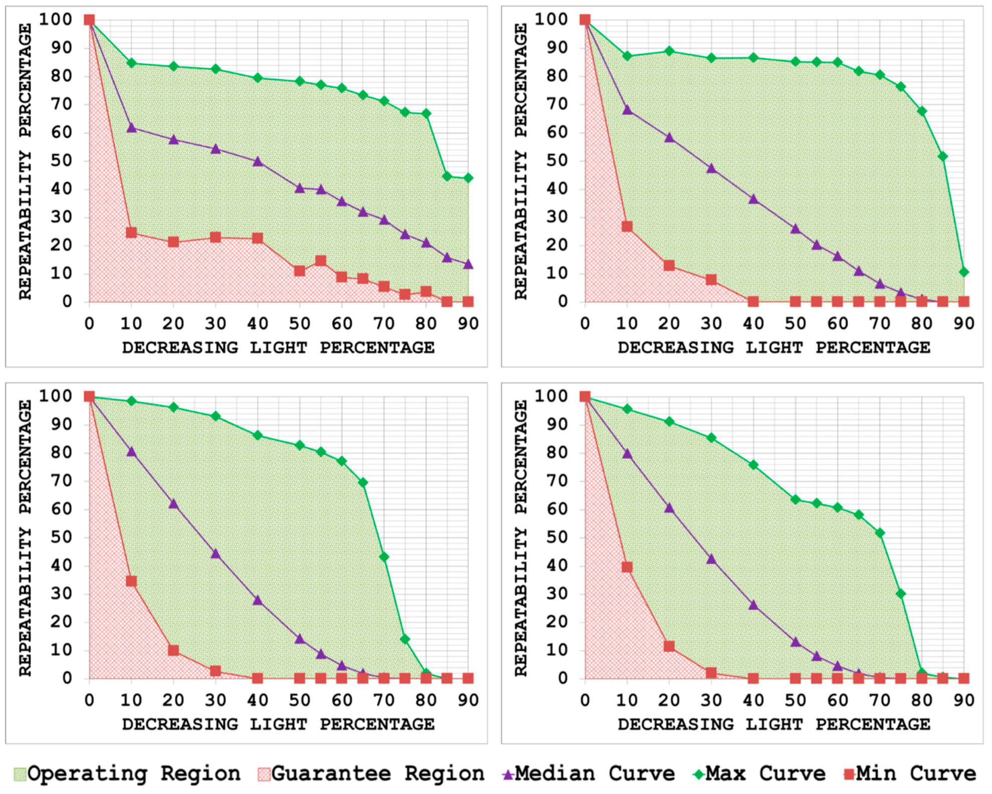
- For every discrete step , the maximum value of repeatability isThe values of set P are plotted against the corresponding image transformation amounts from set A to obtain a curve which represents the upper bound of performance for the given detector with variation in the amount of transformation. This curve is named the max curve.
- (c)
- For every discrete step , the minimum value of repeatability is found to giveThe values of set Q are plotted against the corresponding image transformation amounts from set A to obtain a curve which represents the lower bound of performance for the given detector with the same variations in image transformation. This curve is named the min curve.
- (d)
- For every discrete step , the median value of repeatability is foundThe values of set S are plotted against the corresponding image transformation amounts from set A to obtain a curve which represents the typical performance for the given detector with variation in image transformation amount. This curve is named the median curve.
- (e)
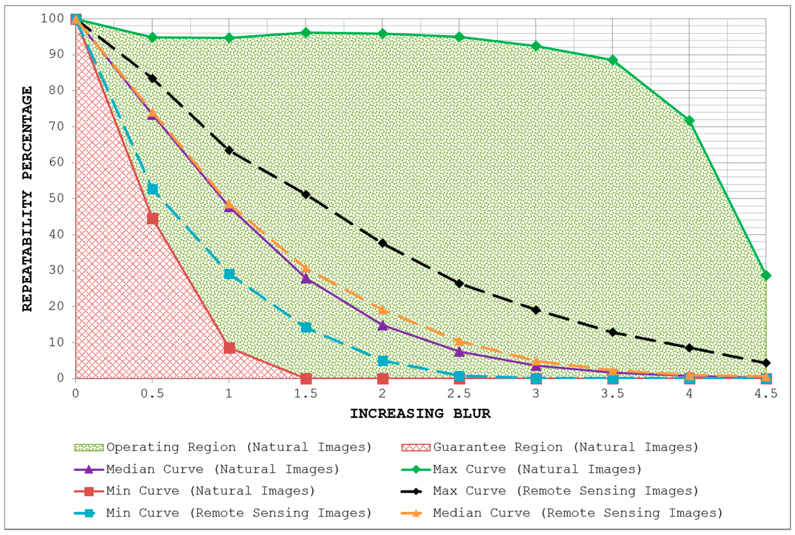
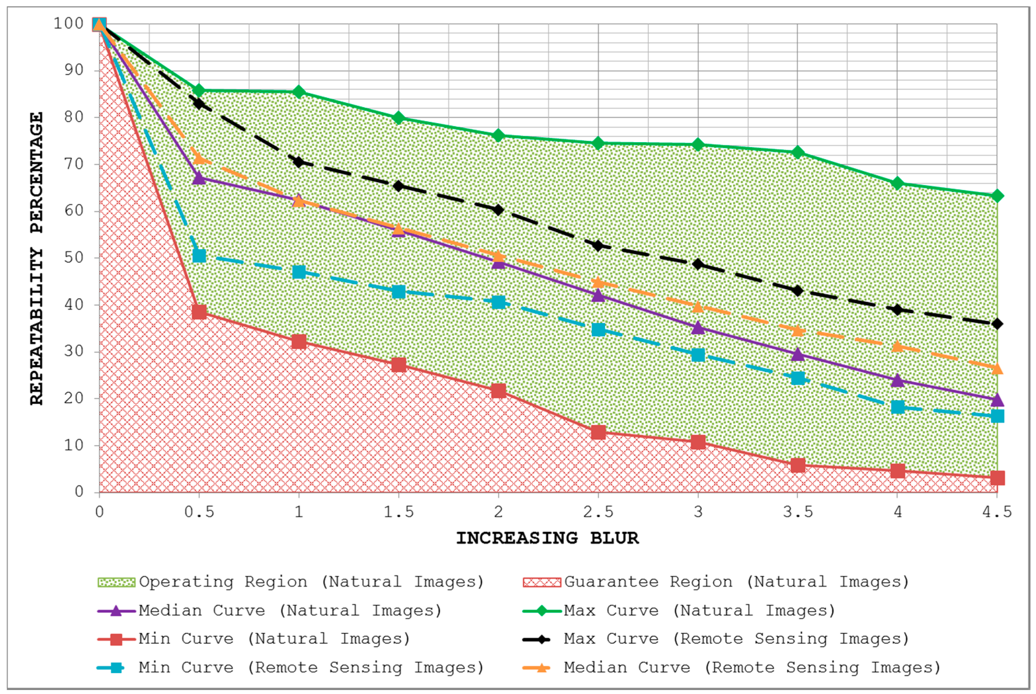
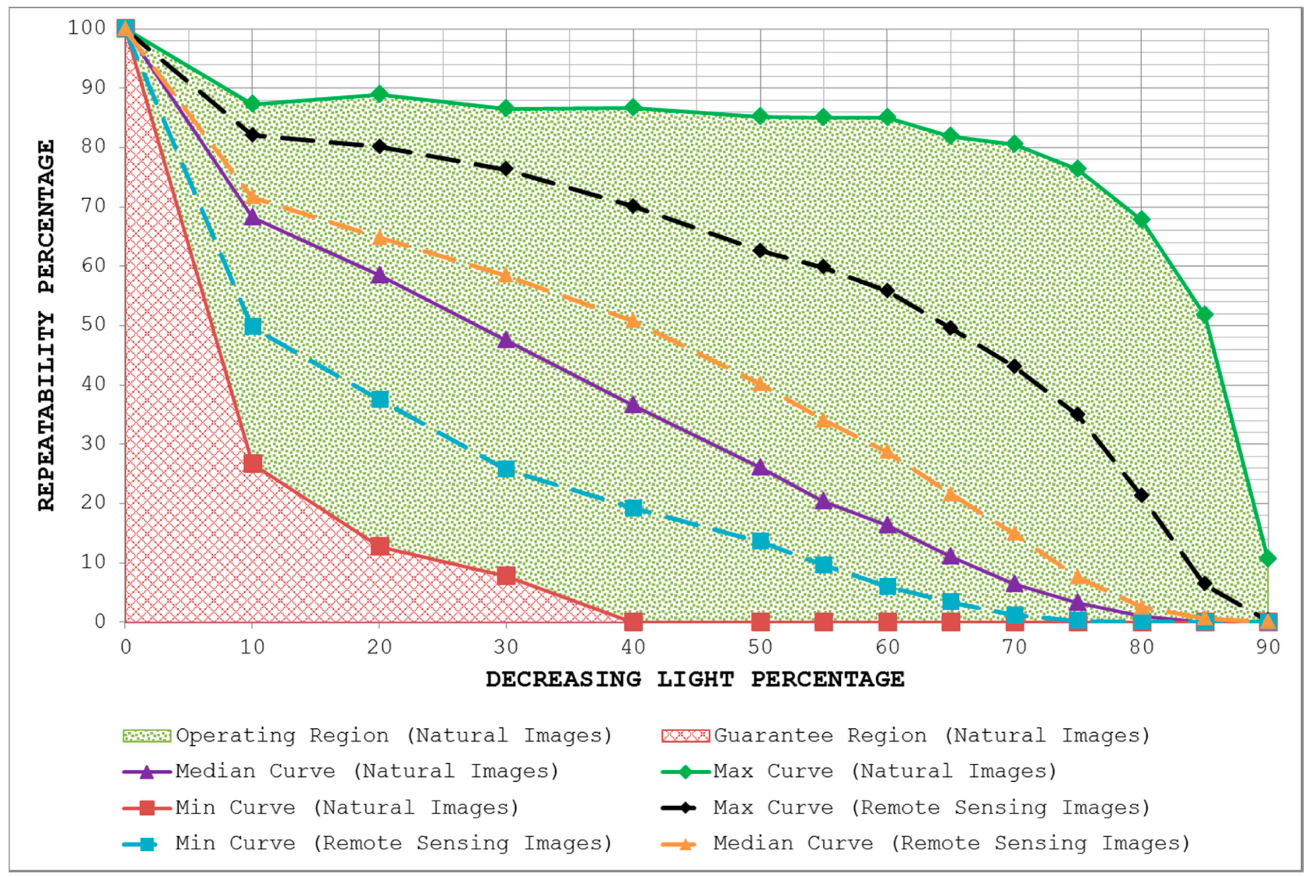
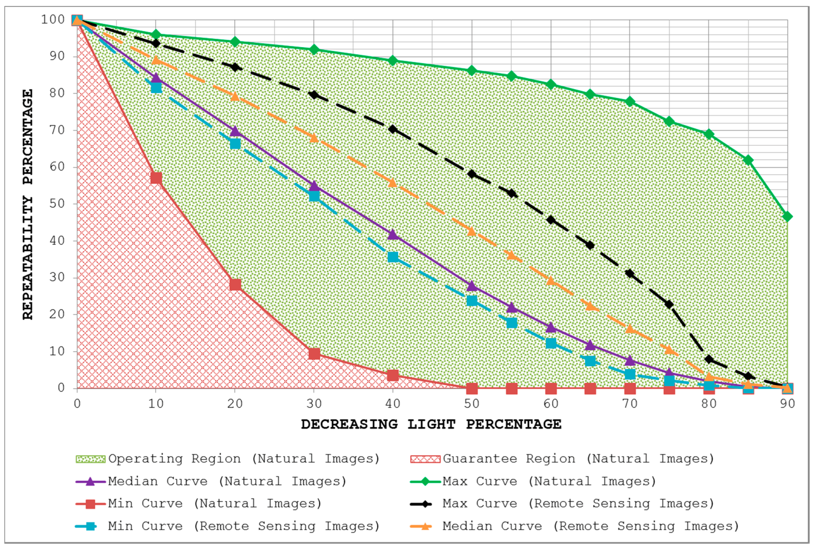
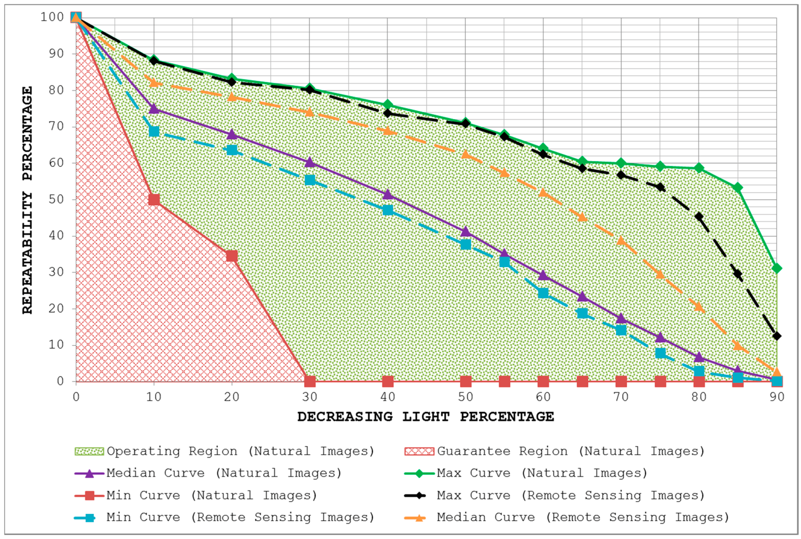
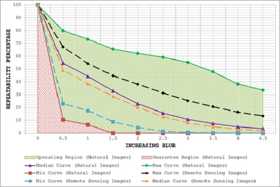
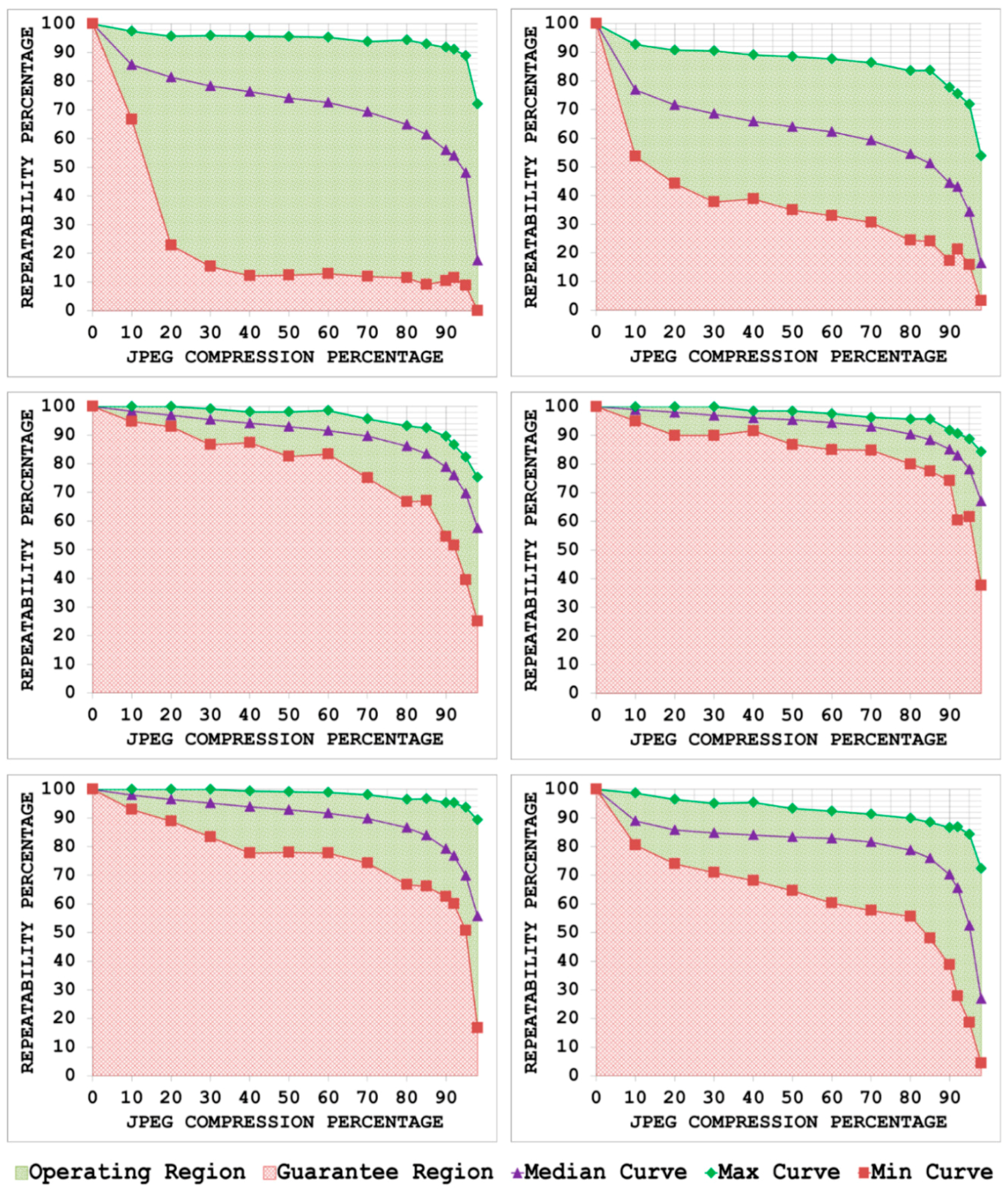
- By plotting the three curves together, the area between the max curve and the min curve is defined as the operating region of the detector. The detector is expected to produce repeatability scores that lie inside this region. A narrow operating region implies that the detector is stable and there is little variation between the maximum and minimum repeatability values that it can achieve for some specific amount of transformation. On the other hand, a large operating region indicates an unstable detector which may achieve high repeatability scores for some particular images but may fare poorly for others.
- (f)
- The area under the min curve is defined as the guarantee region of the detector. Repeatability values achieved by the detector should never be as low so as to lie inside this region. A wide guarantee region shows that the detector manages to achieve reasonably high repeatability values for every input image with increasing amount of image transformation. Contrary to that, a small guarantee region implies that the detector performs poorly with increasing amount of image transformation.
3.2. Phase 2: Identification of Statistically Significant Performance Differences
4. The Image Database
4.1. JPEG Compression
4.2. Blur Changes
4.3. Uniform Light Changes
5. Establishing Operating and Guarantee Regions
5.1. JPEG Compression
5.2. Blur Changes
5.3. Uniform Light Changes
6. Identifying Statistically Significant Performance Differences
6.1. JPEG Compression
6.2. Blur Changes
6.3. Uniform Light Changes
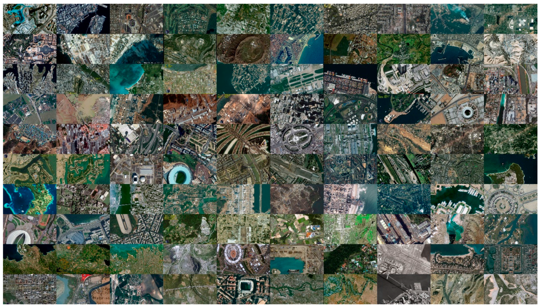
7. Potential for Remote Sensing Applications
8. Conclusions
Acknowledgments
Author Contributions
Conflicts of Interest
References
- Mikolajczyk, K.; Tuytelaars, T.; Schmid, C.; Zisserman, A.; Matas, J.; Schaffalitzky, F.; Kadir, T.; Gool, L.V. A Comparison of Affine Region Detectors. Int. J. Comput. Vis. 2005, 65, 43–72. [Google Scholar] [CrossRef]
- Oxford Data Sets. Available online: http://www.robots.ox.ac.uk/~vgg/research/affine/ (accessed on 5 April 2016).
- Matas, J.; Chum, O.; Urban, M.; Pajdla, T. Robust Wide Baseline Stereo from Maximally Stable Extremal Regions. In Proceedings of the British Machine Vision Conference, Cardiff, UK, 2–5 September 2002; pp. 384–393.
- Torralba, A.; Efros, A.A. Unbiased Look at Dataset Bias. In Proceedings of the Conference on Computer Vision and Pattern Recognition, Colorado Springs, CO, USA, 20–25 June 2011; pp. 1521–1528.
- Ehsan, S.; Kanwal, N.; Clark, A.F.; McDonald-Maier, K.D. Improved Repeatability Measures for Evaluating Performance of Feature Detectors. Electron. Lett. 2010, 46, 998–1000. [Google Scholar] [CrossRef]
- McNemar, Q. Note on the Sampling Error of the Difference between Correlated Proportions or Percentages. Psychometrika 1947, 12, 153–157. [Google Scholar] [CrossRef] [PubMed]
- Fleiss, J.L.; Levin, B.; Paik, M.C. Statistical Methods for Rates and Proportions, 3rd ed.; John Wiley & Sons: New York, NY, USA, 2003. [Google Scholar]
- Rutkowski, W.S.; Rosenfeld, A. A Comparison of Corner Detection Techniques for Chain Coded Curves; Technical Report; University of Maryland: College Park, MD, USA, 1978. [Google Scholar]
- Kitchen, L.; Rosenfeld, A. Gray-Level Corner Detection. Pattern Recognit. Lett. 1982, 1, 95–102. [Google Scholar] [CrossRef]
- Teh, C.H.; Chin, R.T. On the Detection of Dominant Points on Digital Curves. IEEE Trans. Pattern Anal. Mach. Intell. 1989, 11, 859–872. [Google Scholar] [CrossRef]
- Coelho, C.; Heller, A.; Mundy, J.L.; Forsyth, D.A.; Zisserman, A. An Experimental Evaluation of Projective Invariants. In Proceedings of the DARPA-ESPRIT Workshop on Applications of Invariants in Computer Vision, Reykjavik, Iceland, 25–28 March 1991; pp. 273–293.
- Deriche, R.; Giraudon, G. A Computational Approach for Corner and Vertex Detection. Int. J. Comput. Vis. 1993, 10, 101–124. [Google Scholar] [CrossRef]
- Rohr, K. Localization Properties of Direct Corner Detectors. J. Math. Imaging Vis. 1994, 4, 139–150. [Google Scholar] [CrossRef]
- Brand, P.; Mohr, R. Accuracy in Image Measure. In Proceedings of the SPIE Conference on Videometrics III, Boston, MA, USA, 6 October 1994; pp. 218–228.
- Heyden, A.; Rohr, K. Evaluation of Corner Extraction Schemes using Invariance Methods. In Proceedings of the 13th International Conference on Pattern Recognition, Vienna, Austria, 25–29 August 1996; pp. 895–899.
- Heath, M.D.; Sarkar, S.; Sanocki, T.; Bowyer, K.W. A Robust Visual Method for Assessing the Relative Performance of Edge-Detection Algorithms. IEEE Trans. Pattern Anal. Mach. Intell. 1997, 19, 1338–1359. [Google Scholar] [CrossRef]
- Canny, J. A Computational Approach to Edge Detection. IEEE Trans. Pattern Anal. Mach. Intell. 1986, 8, 679–698. [Google Scholar] [CrossRef] [PubMed]
- Demigny, D.; Kamlé, T. A Discrete Expression of Canny’s Criteria for Step Edge Detector Performances Evaluation. IEEE Trans. Pattern Anal. Mach. Intell. 1997, 19, 1199–1211. [Google Scholar] [CrossRef]
- Shin, M.C.; Goldgof, D.; Bowyer, K.W. An Objective Comparison Methodology of Edge Detection Algorithms using a Structure from Motion Task. In Proceedings of the Conference on Computer Vision and Pattern Recognition, Santa Barbara, CA, USA, 25 June 1998; pp. 190–195.
- Shin, M.C.; Goldgof, D.; Bowyer, K.W. Comparison of Edge Detectors using an Object Recognition Task. In Proceedings of the Conference on Computer Vision and Pattern Recognition, Fort Collins, CO, USA, 23–25 June 1999; pp. 360–365.
- Bowyer, K.; Kranenburg, C.; Dougherty, S. Edge Detector Evaluation using Empirical ROC Curves. In Proceedings of the Conference on Computer Vision and Pattern Recognition, Fort Collins, CO, USA, 23–25 June 1999; pp. 354–359.
- Baker, S.; Nayar, S.K. Global Measures of Coherence for Edge Detector Evaluation. In Proceedings of the Conference on Computer Vision and Pattern Recognition, Fort Collins, CO, USA, 23–25 June 1999; pp. 373–379.
- Lopez, A.M.; Lumbreras, F.; Serrat, J.; Villanueva, J.J. Evaluation of Methods for Ridge and Valley Detection. IEEE Trans. Pattern Anal. Mach. Intell. 1999, 21, 327–335. [Google Scholar] [CrossRef]
- Schmid, C.; Mohr, R.; Bauckhage, C. Evaluation of Interest Point Detectors. Int. J. Comput. Vis. 2000, 37, 151–172. [Google Scholar] [CrossRef]
- Sebe, N.; Tian, Q.; Loupias, E.; Lew, M.; Huang, T. Evaluation of Salient Point Techniques. Image Vis. Comput. 2003, 21, 1087–1095. [Google Scholar] [CrossRef]
- Mikolajczyk, K.; Schmid, C. Scale & Affine Invariant Interest Point Detectors. Int. J. Comput. Vis. 2004, 60, 63–86. [Google Scholar]
- Mohanna, F.; Mokhtarian, F. Performance Evaluation of Corner Detection Algorithms under Similarity and Affine Transforms. In Proceedings of the British Machine Vision Conference, Manchester, UK, 10–13 September 2001; pp. 353–362.
- Mokhtarian, F.; Mohanna, F. Performance Evaluation of Corner Detectors using Consistency and Accuracy Measures. Comput. Vis. Image Underst. 2006, 102, 81–94. [Google Scholar] [CrossRef]
- Trajković, M.; Hedley, M. Fast Corner Detection. Image Vis. Comput. 1998, 16, 75–87. [Google Scholar] [CrossRef]
- Tissainayagam, P.; Suter, D. Assessing the Performance of Corner Detectors for Point Feature Tracking Applications. Image Vis. Comput. 2004, 22, 663–679. [Google Scholar] [CrossRef]
- Fraundorfer, F.; Bischof, H. Evaluation of Local Detectors on Non-Planar Scenes. In Proceedings of the Austrian Association for Pattern Recognition Workshop, Hagenberg, Austria, June 2004; pp. 125–132.
- Fraundorfer, F.; Bischof, H. A Novel Performance Evaluation Method of Local Detectors on Non-Planar Scenes. In Proceedings of the IEEE Computer Society Conference on Computer Vision and Pattern Recognition, San Diego, CA, USA, 20–25 June 2005.
- Ehsan, S.; Kanwal, N.; Clark, A.F.; McDonald-Maier, K.D. Measuring the Coverage of Interest Point Detectors. In Proceedings of the 8th International Conference on Image Analysis and Recognition (ICIAR), Burnaby, BC, Canada, 22–24 June 2011; pp. 253–261.
- Ehsan, S.; Clark, A.F.; McDonald-Maier, K.D. Rapid Online Analysis of Local Feature Detectors and their Complementarity. Sensors 2013, 13, 10876–10907. [Google Scholar] [CrossRef] [PubMed]
- Moreels, P.; Perona, P. Evaluation of Features Detectors and Descriptors Based on 3D Objects. In Proceedings of the International Conference on Computer Vision (ICCV), Beijing, China, 17–25 October 2005; pp. 800–807.
- Moreels, P.; Perona, P. Evaluation of features detectors and descriptors based on 3D objects. Int. J. Comput. Vis. 2007, 73, 263–284. [Google Scholar] [CrossRef]
- Mikolajczyk, K.; Leibe, B.; Schiele, B. Local Features for Object Class Recognition. In Proceedings of the International Conference on Computer Vision (ICCV), Beijing, China, 17–25 October 2005; pp. 1792–1799.
- Stark, M.; Schiele, B. How Good are Local Features for Classes of Geometric Objects. In Proceedings of the International Conference on Computer Vision, Rio de Janeiro, Brazil, 14–21 October 2007.
- Seemann, E.; Leibe, B.; Mikolajczyk, K.; Schiele, B. An Evaluation of Local Shape-based Features for Pedestrian Detection. In Proceedings of the British Machine Vision Conference, Oxford, UK, 5–8 September 2005; pp. 11–20.
- Dickscheid, T.; Förstner, W. Evaluating the Suitability of Feature Detectors for Automatic Image Orientation Systems. In Proceedings of the ICVS, Liege, Belgium, 13–15 October 2009; pp. 305–314.
- Haja, A.; Jahne, B.; Abraham, S. Localization Accuracy of Region Detectors. In Proceedings of the IEEE Conference on Computer Vision and Pattern Recognition, Anchorage, AK, USA, 23–28 June 2008.
- Zeisl, B.; Georgel, P.; Schweiger, F.; Steinbach, E.; Navab, N.; Munich, G. Estimation of Location Uncertainty for Scale Invariant Feature Points. In Proceedings of the British Machine Vision Conference, London, UK, 7–10 September 2009.
- Dickscheid, T.; Schindler, F.; Förstner, W. Coding Images with Local Features. Int. J. Comput. Vis. 2010, 94, 154–174. [Google Scholar] [CrossRef]
- Förstner, W.; Dickscheid, T.; Schindler, F. On the Completeness of Coding with Image Features. In Proceedings of the British Machine Vision Conference, London, UK, 7–10 September 2009.
- Aanæs, H.; Dahl, A.L.; Pedersen, K.S. Interesting Interest Points-A Comparative Study of Interest Point Performance on a Unique Data Set. Int. J. Comput. Vis. 2012, 97, 18–35. [Google Scholar] [CrossRef]
- Lowe, D.G. Object Recognition from Local Scale-Invariant Features. In Proceedings of the International Conference on Computer Vision, Corfu, Greece, 30 September–2 October 1999; pp. 1150–1157.
- Lowe, D.G. Distinctive Image Features from Scale-Invariant Keypoints. Int. J. Comput. Vis. 2004, 60, 91–110. [Google Scholar] [CrossRef]
- Gil, A.; Mozos, O.M.; Ballesta, M.; Reinoso, O. A Comparative Evaluation of Interest Point Detectors and Local Descriptors for Visual SLAM. Mach. Vis. Appl. 2010, 21, 905–920. [Google Scholar] [CrossRef]
- Asbach, M.; Hosten, P.; Unger, M. An Evaluation of Local Features for Face Detection and Localization. In Proceedings of the Ninth International Workshop on Image Analysis for Multimedia Interactive Services, Klagenfurt, Austria, 7–9 May 2008; pp. 32–35.
- JPEG, Blurring and Uniform Light Changes Image Database. Available online: http://vase.essex.ac.uk/datasets/index.html (accessed on 15 April 2016).
- Bay, H.; Ess, A.; Tuytelaars, T.; Gool, L.V. Speeded-Up Robust Features (SURF). Comput. Vis. Image Underst. 2008, 110, 346–359. [Google Scholar] [CrossRef]
- Tuytelaars, T.; Gool, L.V. Matching Widely Separated Views Based on Affine Invariant Regions. Int. J. Comput. Vis. 2004, 59, 61–85. [Google Scholar] [CrossRef]
- Forstner, W.; Dickscheid, T.; Schindler, F. Detecting Interpretable and Accurate Scale-Invariant Keypoints. In Proceedings of the 12th IEEE International Conference on Computer Vision, Kyoto, Japan, 27 September–4 October 2009; pp. 2256–2263.
- Kadir, T.; Zisserman, A.; Brady, M. An Affine Invariant Salient Region Detector. In Proceedings of the 8th European Conference on Computer Vision, Prague, Czech Republic, 11–14 May 2004; pp. 228–241.
- Tuytelaars, T.; Mikolajczyk, K. Local Invariant Feature Detectors: A Survey. Found. Trends Comput. Graph. Vis. 2007, 3, 177–280. [Google Scholar] [CrossRef]
- Remote Sensing Images. Available online: http://www.satimagingcorp.com/ (accessed on 10 October 2016).


| S. No. | Feature Detector | Parameter Settings |
|---|---|---|
| 1 | EBR | scalefactor = 1.0 |
| 2 | IBR | scalefactor = 1.0 |
| 3 | MSER | t = 2; es = 2 |
| 4 | SIFT | edge_thresh = −1; peak_thresh = −1; magnif = −1; O = −1; S = 3; omin = −1; |
| 5 | SURF | samplingStep = 2; octaves = 4; thres = 4.0; doubleImageSize = 0; initLobe = 3; |
| 6 | SFOP | layersPerOctave = 4; numberOfOctaves = 3; Tp = −Inf; Tlambda2 = 2; noise = 0.02; nonmaxTd2 = 1; nonmaxOctave = 0.5; sizeFactor = 1; koetheMaxIter = 5; koetheEpsilon = 0.2; |
| 7 | HARLAP | thres = 1000 |
| 8 | HARAFF | thres = 1000 |
| 9 | HESLAP | thres = 500 |
| 10 | HESAFF | thres = 500 |
| 11 | SALIENT | StartScale = 3; StopScale = 33; AA = 0; Nbins = 16; Sigma = 1; div= 16; wt = 0.5; yt = 0; |
© 2016 by the authors; licensee MDPI, Basel, Switzerland. This article is an open access article distributed under the terms and conditions of the Creative Commons Attribution (CC-BY) license (http://creativecommons.org/licenses/by/4.0/).
Share and Cite
Ehsan, S.; Clark, A.F.; Leonardis, A.; Ur Rehman, N.; Khaliq, A.; Fasli, M.; McDonald-Maier, K.D. A Generic Framework for Assessing the Performance Bounds of Image Feature Detectors. Remote Sens. 2016, 8, 928. https://doi.org/10.3390/rs8110928
Ehsan S, Clark AF, Leonardis A, Ur Rehman N, Khaliq A, Fasli M, McDonald-Maier KD. A Generic Framework for Assessing the Performance Bounds of Image Feature Detectors. Remote Sensing. 2016; 8(11):928. https://doi.org/10.3390/rs8110928
Chicago/Turabian StyleEhsan, Shoaib, Adrian F. Clark, Ales Leonardis, Naveed Ur Rehman, Ahmad Khaliq, Maria Fasli, and Klaus D. McDonald-Maier. 2016. "A Generic Framework for Assessing the Performance Bounds of Image Feature Detectors" Remote Sensing 8, no. 11: 928. https://doi.org/10.3390/rs8110928
APA StyleEhsan, S., Clark, A. F., Leonardis, A., Ur Rehman, N., Khaliq, A., Fasli, M., & McDonald-Maier, K. D. (2016). A Generic Framework for Assessing the Performance Bounds of Image Feature Detectors. Remote Sensing, 8(11), 928. https://doi.org/10.3390/rs8110928