
Direct Measurements of Bedrock Incision Rates on the Surface of a Large Dip-slope Landslide by Multi-Period Airborne Laser Scanning DEMs

 , , and
Abstract
:
1. Introduction
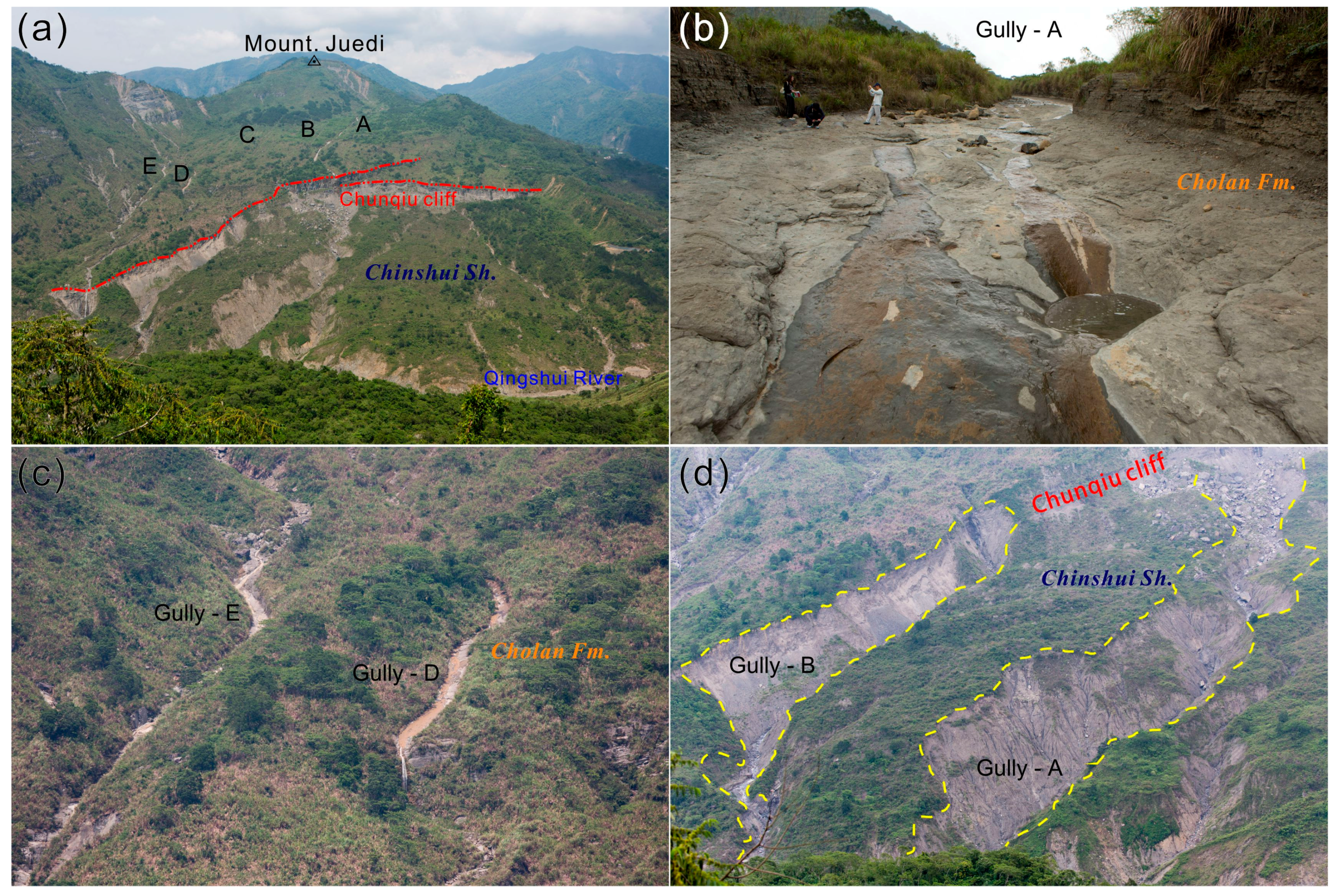
2. Study Area
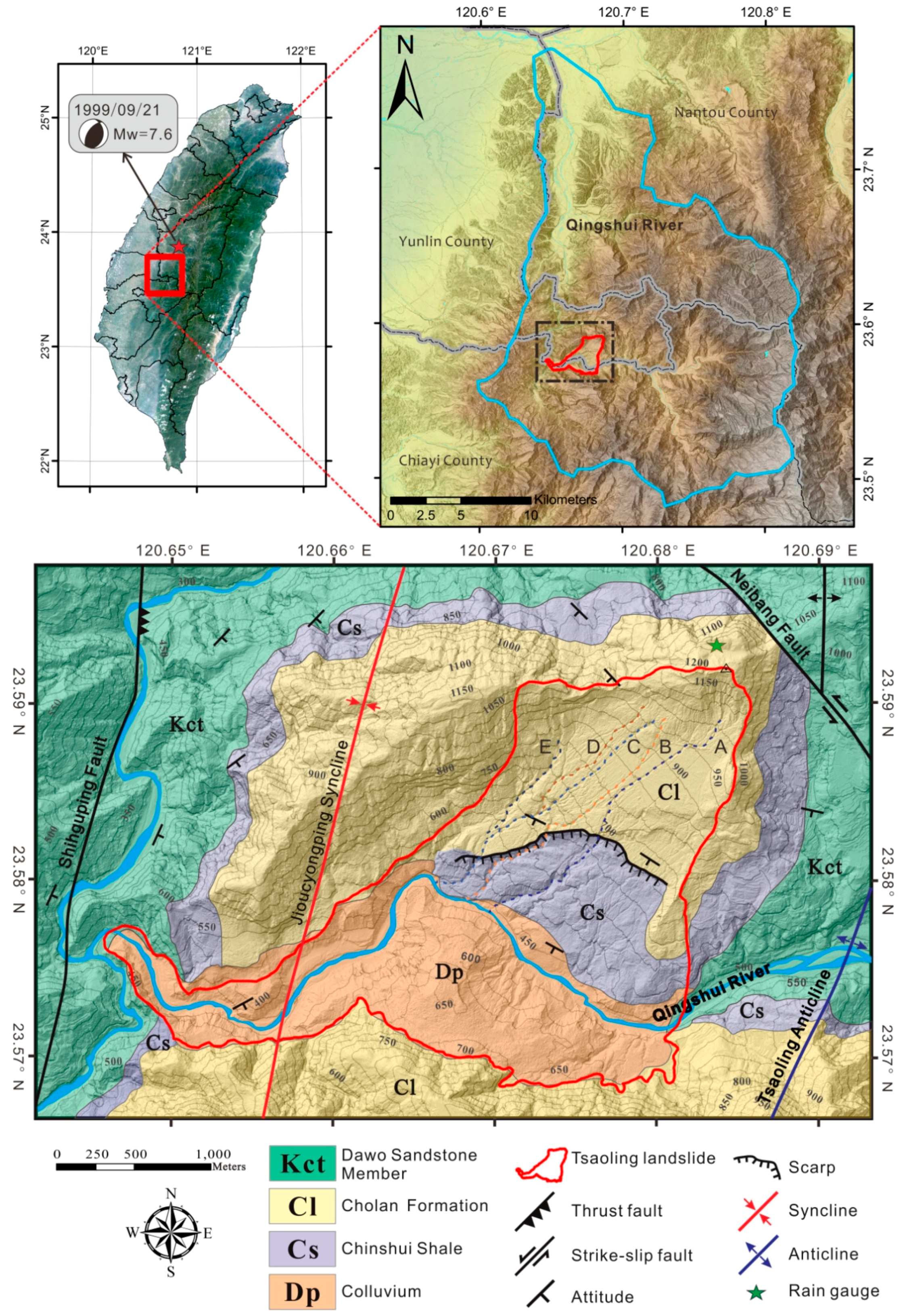
2.1. Geological Setting
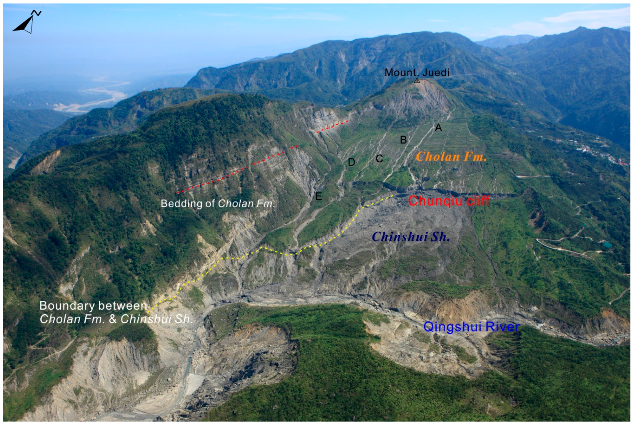
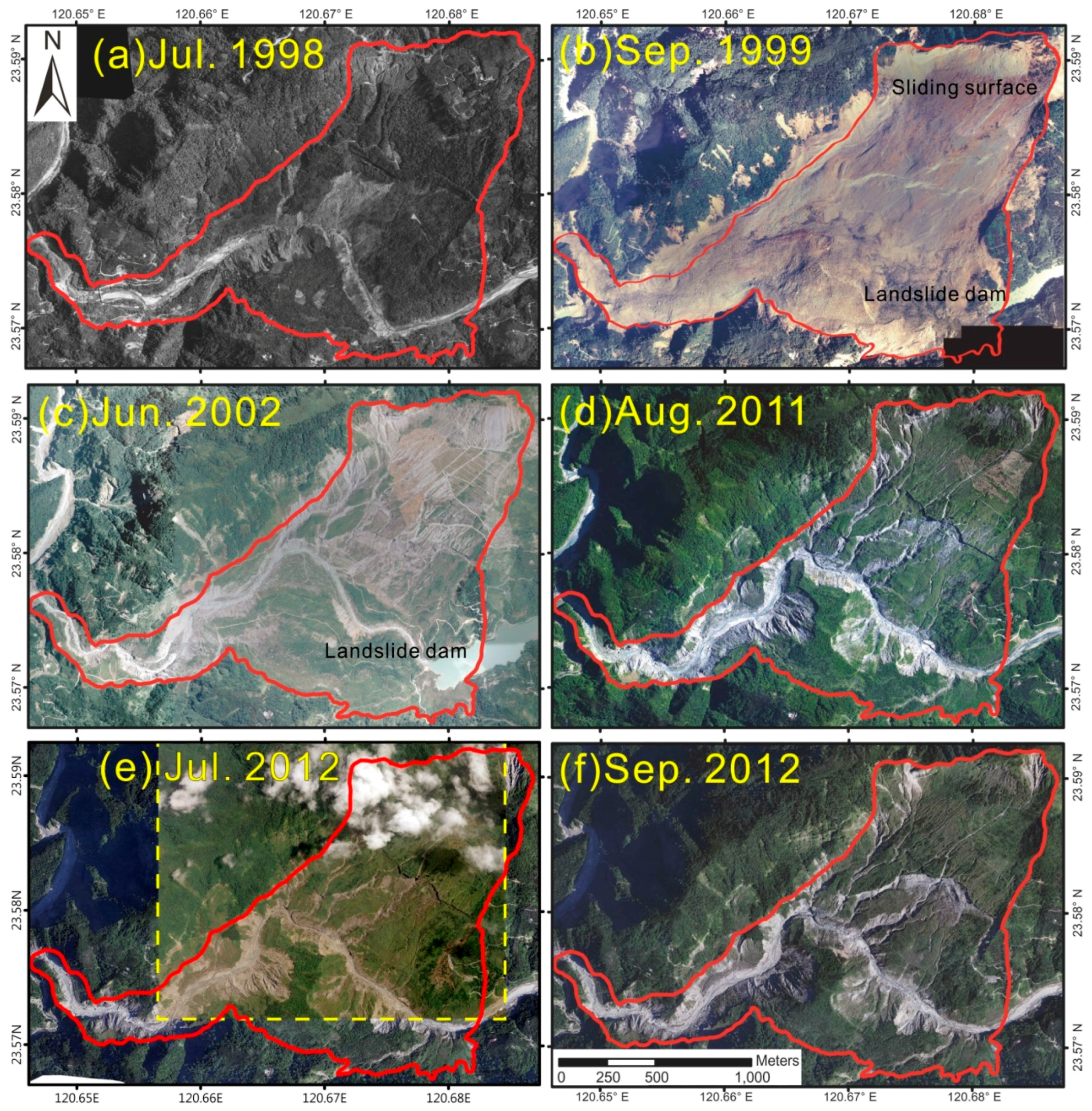
2.2. Overview of Tsaoling Landslide
3. Materials and Methods
3.1. Airborne Laser Scanning (ALS)
3.2. Aerial Photogrammetry
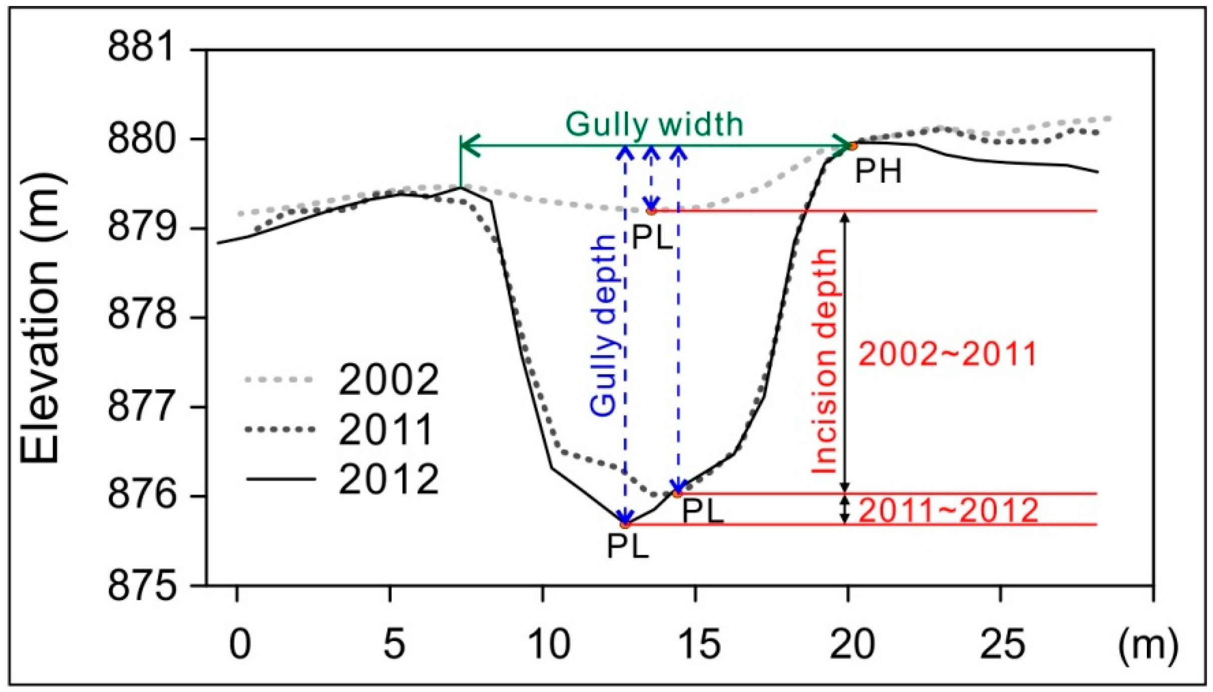
3.3. Calculation Methods for Gully Incision Depth
3.3.1. Equal-Interval Cross Section Selection Method
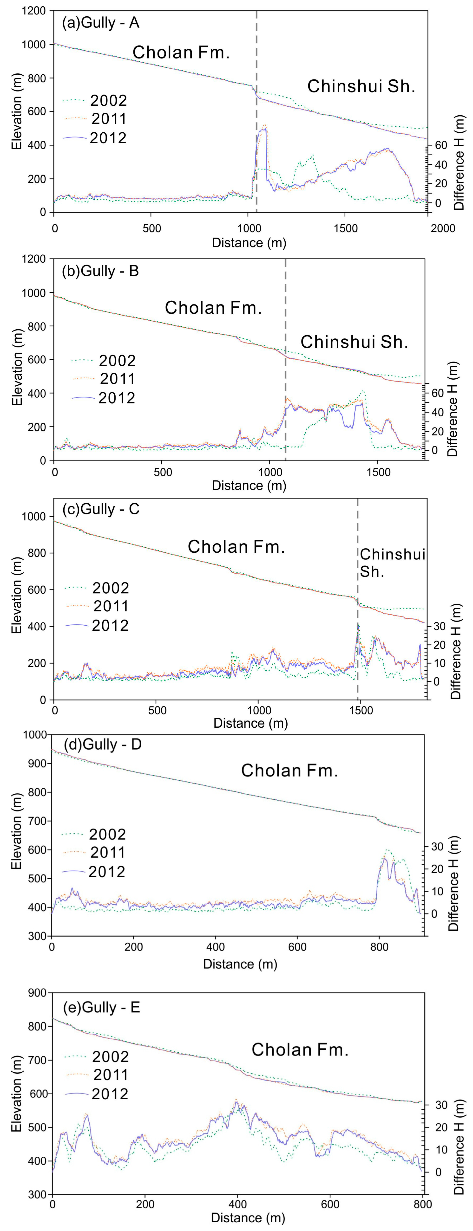
3.3.2. Continuous Swath Profiles Selection Method
4. Results
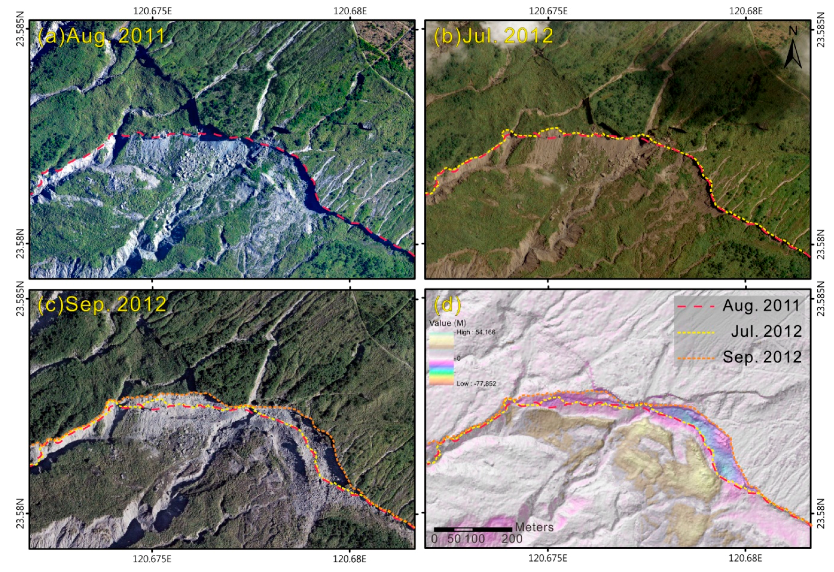
4.1. Image Interpretation Results
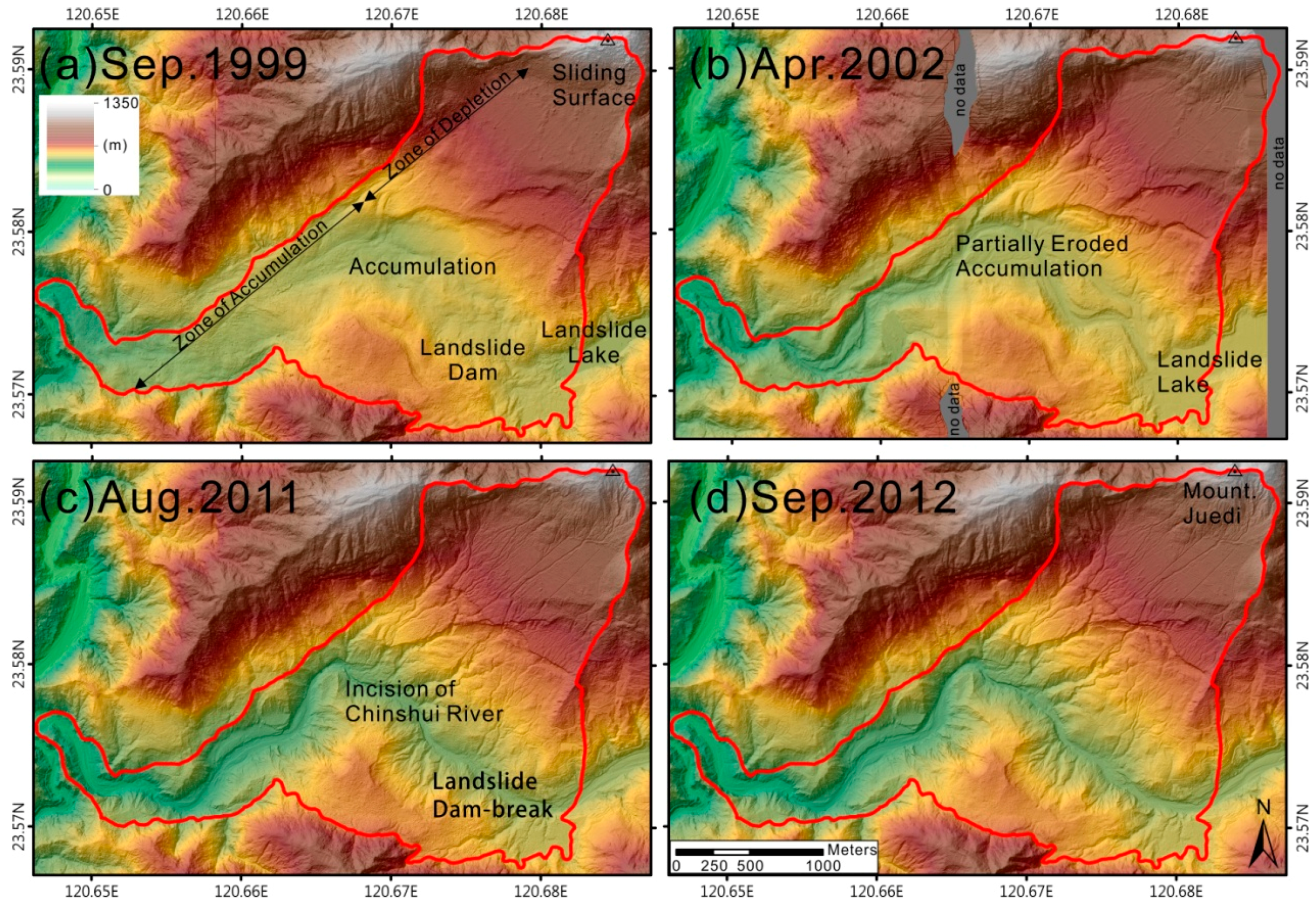
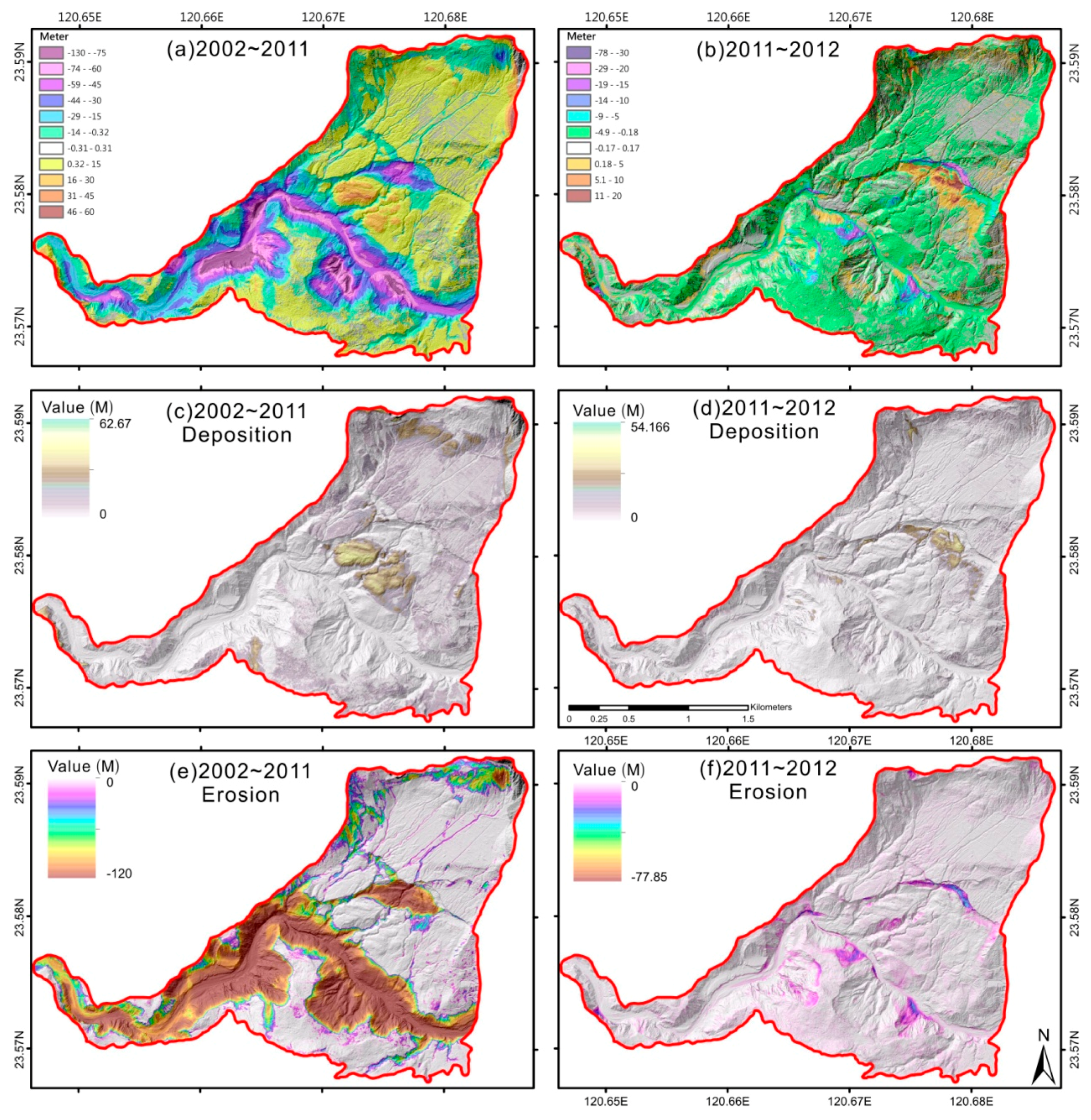
4.2. DEM Topographic Interpretation
4.3. Calculations of Incision Rates
4.3.1. The Equal-Interval Cross Section Selection Method
4.3.2. The Continuous Swath Profiles Selection Method
4.4. Three-Period ALS DEM Data Comparison and Error Estimation
5. Discussion
5.1. Three-Period Data Comparison and Error Evaluation
5.2. Gully Incision Rate
5.3. Continuous Sampling and Intermittent Sampling
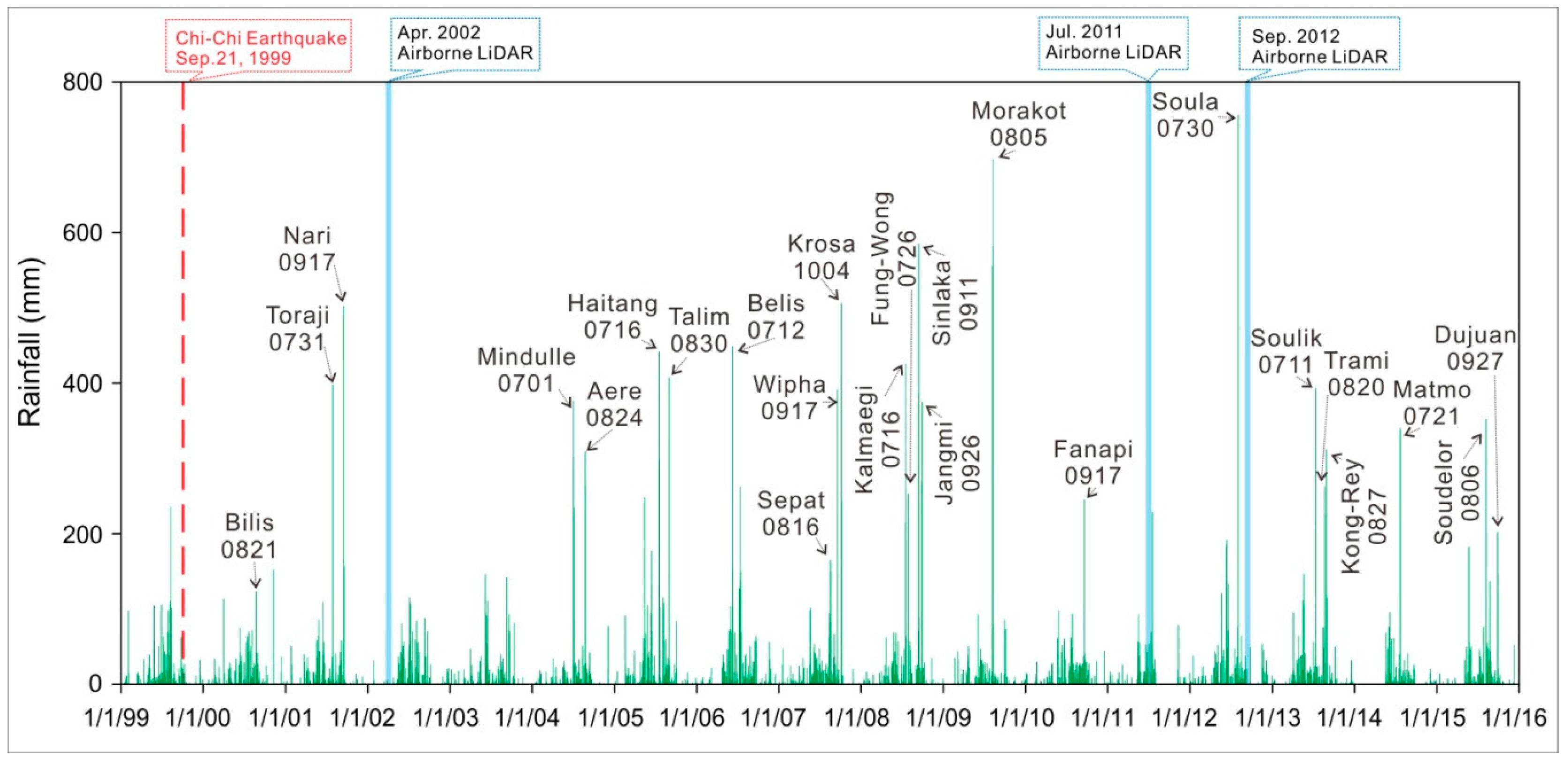
5.4. The Effects of Typhoon Soula
5.5. Gully Bedrock Incision Rate
6. Conclusions
Acknowledgments
Author Contributions
Conflicts of Interest
References
- Chang, K.-J.; Taboada, A.; Chan, Y.-C. Geological and morphological study of the Jiufengershan landslide triggered by the Chi-Chi Taiwan earthquake. Geomorphology 2005, 71, 293–309. [Google Scholar] [CrossRef]
- Chen, R.-F.; Chang, K.-J.; Angelier, J.; Chan, Y.-C.; Deffontaines, B.; Lee, C.-T.; Lin, M.-L. Topographical changes revealed by high-resolution airborne LiDAR data: The 1999 Tsaoling landslide induced by the Chi–Chi earthquake. Eng. Geol. 2006, 88, 160–172. [Google Scholar] [CrossRef]
- Corsini, A.; Borgatti, L.; Cervi, F.; Dahne, A.; Ronchetti, F.; Sterzai, P. Estimating mass-wasting processes in active earth slides—Earth flows with time-series of High-Resolution DEMs from photogrammetry and airborne LiDAR. Nat. Hazards Earth Syst. Sci. 2009, 9, 433–439. [Google Scholar] [CrossRef]
- DeLong, S.B.; Prentice, C.S.; Hilley, G.E.; Ebert, Y. Multitemporal ALSM change detection, sediment delivery, and process mapping at an active earthflow. Earth Surf. Process. Landf. 2012, 37, 262–272. [Google Scholar] [CrossRef]
- Huang, Y.; Yu, M.; Xu, Q.; Sawada, K.; Moriguchi, S.; Yashima, A.; Liu, C.; Xue, L. InSAR-derived digital elevation models for terrain change analysis of earthquake-triggered flow-like landslides based on ALOS/PALSAR imagery. Environ. Earth Sci. 2014, 73, 7661–7668. [Google Scholar] [CrossRef]
- Roering, J.J.; Stimely, L.L.; Mackey, B.H.; Schmidt, D.A. Using DInSAR, airborne LiDAR, and archival air photos to quantify landsliding and sediment transport. Geophys. Res. Lett. 2009, 36. [Google Scholar] [CrossRef]
- Derose, R.C.; Gomez, B.; Marden, M.; Trustrum, N.A. Gully erosion in Mangatu Forest, New Zealand, estimated from digital elevation models. Earth Surf. Process. Landf. 1998, 23, 1045–1053. [Google Scholar] [CrossRef]
- Grove, J.R.; Croke, J.; Thompson, C. Quantifying different riverbank erosion processes during an extreme flood event. Earth Surf. Process. Landf. 2013, 38, 1393–1406. [Google Scholar] [CrossRef]
- Heritage, G.; Hetherington, D. Towards a protocol for laser scanning in fluvial geomorphology. Earth Surf. Process. Landf. 2007, 32, 66–74. [Google Scholar] [CrossRef]
- Dewitte, O.; Jasselette, J.C.; Cornet, Y.; Van Den Eeckhaut, M.; Collignon, A.; Poesen, J.; Demoulin, A. Tracking landslide displacements by multi-temporal DTMs: A combined aerial stereophotogrammetric and LiDAR approach in western Belgium. Eng. Geol. 2008, 99, 11–22. [Google Scholar] [CrossRef]
- Hsieh, Y.-C.; Chan, Y.-C.; Hu, J.-C. Digital elevation model differencing and error estimation from multiple sources: A case study from the Meiyuan Shan landslide in Taiwan. Remote Sens. 2016, 8, 199. [Google Scholar] [CrossRef]
- Milan, D.J.; Heritage, G.L.; Hetherington, D. Application of a 3D laser scanner in the assessment of erosion and deposition volumes and channel change in a proglacial river. Earth Surf. Process. Landf. 2007, 32, 1657–1674. [Google Scholar] [CrossRef]
- Ventura, G.; Vilardo, G.; Terranova, C.; Sessa, E.B. Tracking and evolution of complex active landslides by multi-temporal airborne LiDAR data: The Montaguto landslide (Southern Italy). Remote Sens. Environ. 2011, 115, 3237–3248. [Google Scholar] [CrossRef]
- Tarolli, P. High-resolution topography for understanding Earth surface processes: Opportunities and challenges. Geomorphology 2014, 216, 295–312. [Google Scholar] [CrossRef]
- Collins, B.D.; Montgomery, D.R.; Schanz, S.A.; Larsen, I.J. Rates and mechanisms of bedrock incision and strath terrace formation in a forested catchment, Cascade Range, Washington. Geol. Soc. Am. Bull. 2016, 128, 926–943. [Google Scholar] [CrossRef]
- Whipple, K.X.; Snyder, N.P.; Dollenmayer, K. Rates and processes of bedrock incision by the Upper Ukak River since the 1912 Novarupta ash flow in the Valley of Ten Thousand Smokes, Alaska. Geology 2000, 28, 835–838. [Google Scholar] [CrossRef]
- Montgomery, D.R. Observations on the role of lithology in strath terrace formation and bedrock channel width. Am. J. Sci. 2004, 304, 454–476. [Google Scholar] [CrossRef]
- Schaller, M.; Hovius, N.; Willett, S.D.; Ivy-Ochs, S.; Synal, H.A.; Chen, M.C. Fluvial bedrock incision in the active mountain belt of Taiwan from in situ-produced cosmogenic nuclides. Earth Surf. Process. Landf. 2005, 30, 955–971. [Google Scholar] [CrossRef]
- Pratt-Sitaula, B.; Garde, M.; Burbank, D.W.; Oskin, M.; Heimsath, A.; Gabet, E. Bedload-to-suspended load ratio and rapid bedrock incision from Himalayan landslide-dam lake record. Quat. Res. 2007, 68, 111–120. [Google Scholar] [CrossRef]
- Liang, H.; Zhang, K.; Fu, J.; Li, L.; Chen, J.; Li, S.; Chen, L. Bedrock river incision response to basin connection along the Jinshan Gorge, Yellow River, North China. J. Asian Earth Sci. 2015, 114, 203–211. [Google Scholar] [CrossRef]
- Finnegan, N.J.; Schumer, R.; Finnegan, S. A signature of transience in bedrock river incision rates over timescales of 104–107 years. Nature 2014, 505, 391–394. [Google Scholar] [CrossRef] [PubMed]
- Reusser, L.J.; Bierman, P.R.; Pavich, M.J.; Zen, E.-a.; Larsen, J.; Finkel, R. Rapid Late Pleistocene Incision of Atlantic Passive-Margin River Gorges. Science 2004, 305, 499–502. [Google Scholar] [CrossRef] [PubMed]
- Leland, J.; Reid, M.R.; Burbank, D.W.; Finkel, R.; Caffee, M. Incision and differential bedrock uplift along the Indus River near Nanga Parbat, Pakistan Himalaya, from 10Be and 26Al exposure age dating of bedrock straths. Earth Planet. Sci. Lett. 1998, 154, 93–107. [Google Scholar] [CrossRef]
- Burbank, D.W.; Leland, J.; Fielding, E.; Anderson, R.S.; Brozovic, N.; Reid, M.R.; Duncan, C. Bedrock incision, rock uplift and threshold hillslopes in the northwestern Himalayas. Nature 1996, 379, 505–510. [Google Scholar] [CrossRef]
- Siame, L.L.; Angelier, J.; Chen, R.F.; Godard, V.; Derrieux, F.; Bourlès, D.L.; Braucher, R.; Chang, K.J.; Chu, H.T.; Lee, J.C. Erosion rates in an active orogen (NE-Taiwan): A confrontation of cosmogenic measurements with river suspended loads. Quat. Geochronol. 2011, 6, 246–260. [Google Scholar] [CrossRef]
- Dadson, S.J.; Hovius, N.; Chen, H.; Dade, W.B.; Hsieh, M.-L.; Willett, S.D.; Hu, J.-C.; Horng, M.-J.; Chen, M.-C.; Stark, C.P.; et al. Links between erosion, runoff variability and seismicity in the Taiwan orogen. Nature 2003, 426, 648–651. [Google Scholar] [CrossRef] [PubMed]
- Kao, S.-J.; Liu, K.-K. Exacerbation of erosion induced by human perturbation in a typical Oceania watershed: Insight from 45 years of hydrological records from the Lanyang-Hsi River, northeastern Taiwan. Glob. Biogeochem. Cycles 2002, 16, 16-1–16-7. [Google Scholar] [CrossRef]
- Malik, I. Dating of small gully formation and establishing erosion rates in old gullies under forest by means of anatomical changes in exposed tree roots (Southern Poland). Geomorphology 2008, 93, 421–436. [Google Scholar] [CrossRef]
- Saez, J.L.; Corona, C.; Stoffel, M.; Rovéra, G.; Astrade, L.; Berger, F. Mapping of erosion rates in marly badlands based on a coupling of anatomical changes in exposed roots with slope maps derived from LiDAR data. Earth Surf. Process. Landf. 2011, 36, 1162–1171. [Google Scholar] [CrossRef]
- Perroy, R.L.; Bookhagen, B.; Asner, G.P.; Chadwick, O.A. Comparison of gully erosion estimates using airborne and ground-based LiDAR on Santa Cruz Island, California. Geomorphology 2010, 118, 288–300. [Google Scholar] [CrossRef]
- Goodwin, N.R.; Armston, J.; Stiller, I.; Muir, J. Assessing the repeatability of terrestrial laser scanning for monitoring gully topography: A case study from Aratula, Queensland, Australia. Geomorphology 2016, 262, 24–36. [Google Scholar] [CrossRef]
- Huang, M.-W.; Pan, Y.-W.; Liao, J.-J. A case of rapid rock riverbed incision in a coseismic uplift reach and its implications. Geomorphology 2013, 184, 98–110. [Google Scholar] [CrossRef]
- Cook, K.L.; Turowski, J.M.; Hovius, N. A demonstration of the importance of bedload transport for fluvial bedrock erosion and knickpoint propagation. Earth Surf. Process. Landf. 2013, 38, 683–695. [Google Scholar] [CrossRef]
- Betts, H.D.; DeRose, R.C. Digital elevation models as a tool for monitoring and measuring gully erosion. Int. J. Appl. Earth Obs. Geoinf. 1999, 1, 91–101. [Google Scholar] [CrossRef]
- Evans, M.; Lindsay, J. High resolution quantification of gully erosion in upland peatlands at the landscape scale. Earth Surf. Process. Landf. 2010, 35, 876–886. [Google Scholar] [CrossRef]
- James, L.A.; Watson, D.G.; Hansen, W.F. Using LiDAR data to map gullies and headwater streams under forest canopy: South Carolina, USA. CATENA 2007, 71, 132–144. [Google Scholar] [CrossRef]
- Liu, H.-C.; Lee, J.-F.; Chi, C.-C. Yunlin. In Geological Map of Taiwan Scale 1:50,000, 2nd ed.; Lin, C.-C., Ed.; Central Geological Survey, MOEA: New Taipei City, Taiwan, 2004. [Google Scholar]
- Hsu, T.-L.; Leung, H. Mass movements in the Tsaoling area, Yunlin-Hsien, Taiwan. Proc. Geol. Soc. China 1977, 20, 114–118. [Google Scholar]
- Huang, C.-S.; Ho, H.; Liu, H. The geology and landslide of Tsaoling area, Yunlin, Taiwan. Bull. Cent. Geol. Surv. 1983, 2, 95–112. [Google Scholar]
- Hung, J.-J.; Lee, C.-T.; Lin, M.-L. Tsao-Ling rockslides, Taiwan. Rev. Eng. Geol. 2002, 15, 91–116. [Google Scholar]
- Tang, C.-L.; Hu, J.-C.; Lin, M.-L.; Angelier, J.; Lu, C.-Y.; Chan, Y.-C.; Chu, H.-T. The Tsaoling landslide triggered by the Chi-Chi earthquake, Taiwan: Insights from a discrete element simulation. Eng. Geol. 2009, 106, 1–19. [Google Scholar] [CrossRef]
- Lee, C.-T. Geomorphological evolution and geology of the Tsaoling Rockslide. J. Chin. Soil Water Conserv. 2011, 42, 63–73. [Google Scholar]
- Chigira, M.; Wang, W.-N.; Furuya, T.; Kamai, T. Geological causes and geomorphological precursors of the Tsaoling landslide triggered by the 1999 Chi-Chi earthquake, Taiwan. Eng. Geol. 2003, 68, 259–273. [Google Scholar] [CrossRef]
- Chen, R.-F.; Chan, Y.-C.; Angelier, J.; Hu, J.-C.; Huang, C.; Chang, K.-J.; Shih, T.-Y. Large earthquake-triggered landslides and mountain belt erosion: The Tsaoling case, Taiwan. Comptes Rendus Geoscience 2005, 337, 1164–1172. [Google Scholar] [CrossRef]
- Central Weather Bureau (CWB), R.O.C. Typhoon Database. Available online: http://rdc28.cwb.gov.tw/ (accessed on 15 August 2016).
- Hung, J.-J. Chi-Chi earthquake induced landslides in Taiwan. Earthq. Eng. Eng. Seismol. 2000, 2, 25–33. [Google Scholar]
- Dong, J.-J.; Yang, C.-M.; Yu, W.-L.; Lee, C.-T.; Miyamoto, Y.; Shimamoto, T. Velocity-displacement dependent friction coefficient and the kinematics of giant landslide. In Earthquake-Induced Landslides; Springer: Berlin, Germany, 2013; pp. 397–403. [Google Scholar]
- Chang, K.-J.; Wei, S.-K.; Chen, R.-F.; Chan, Y.-C.; Tsai, P.-W.; Kuo, C.-Y. Empirical modal decomposition of near field seismic signals of Tsaoling landslide. In Earthquake-Induced Landslides; Springer: Berlin, Germany, 2013; pp. 421–430. [Google Scholar]
- Chen, T.C.; Lin, M.L.; Wang, K.L. Landslide seismic signal recognition and mobility for an earthquake-induced rockslide in Tsaoling, Taiwan. Eng. Geol. 2014, 171, 31–44. [Google Scholar] [CrossRef]
- Yang, C.-M.; Yu, W.-L.; Dong, J.-J.; Kuo, C.-Y.; Shimamoto, T.; Lee, C.-T.; Togo, T.; Miyamoto, Y. Initiation, movement, and run-out of the giant Tsaoling landslide—What can we learn from a simple rigid block model and a velocity–displacement dependent friction law? Eng. Geol. 2014, 182, 158–181. [Google Scholar] [CrossRef]
- Kuo, C.Y.; Tai, Y.C.; Bouchut, F.; Mangeney, A.; Pelanti, M.; Chen, R.F.; Chang, K.J. Simulation of Tsaoling landslide, Taiwan, based on Saint Venant equations over general topography. Eng. Geol. 2009, 104, 181–189. [Google Scholar] [CrossRef]
- Peng, M.H.; Shih, T.Y. Error assessment in two LiDAR-derived TIN datasets. Photogramm. Eng. Remote Sens. 2006, 72, 933–947. [Google Scholar] [CrossRef]
- Ministry of the Interior, R.O.C. Establishment of The national coordinate system. Available online: http://gps.moi.gov.tw/SSCenter/Introduce_E/IntroducePage_E.aspx?Page=GPS_E8 (accessed on 15 December 2015).
- Ministry of the Interior, R.O.C. Taiwan Vertical Datum. Available online: http://gps.moi.gov.tw/SSCenter/Introduce_E/IntroducePage_E.aspx?Page=Height_E4 (accessed on 15 December 2015).
- Telbisz, T.; Kovács, G.; Székely, B.; Szabó, J. Topographic swath profile analysis: A generalization and sensitivity evaluation of a digital terrain analysis tool. Z. Geomorphol. 2013, 57, 485–513. [Google Scholar] [CrossRef]
- Hergarten, S.; Robl, J.; Stüwe, K. Extracting topographic swath profiles across curved geomorphic features. Earth Surf. Dynam. 2014, 2, 97–104. [Google Scholar] [CrossRef]
- Benjamin, M.J.; Jason, M.S.; Ann, E.G.; Guido, G.; Vladimir, E.R.; Thomas, A.D.; Nicole, E.M.K.; Bruce, M.R. Quantifying landscape change in an arctic coastal lowland using repeat airborne LiDAR. Environ. Res. Lett. 2013, 8, 045025. [Google Scholar]
- Iverson, R.M.; George, D.L.; Allstadt, K.; Reid, M.E.; Collins, B.D.; Vallance, J.W.; Schilling, S.P.; Godt, J.W.; Cannon, C.M.; Magirl, C.S.; et al. Landslide mobility and hazards: implications of the 2014 Oso disaster. Earth Planet. Sci. Lett. 2015, 412, 197–208. [Google Scholar] [CrossRef]
- Rumsby, B.; Brasington, J.; Langham, J.; McLelland, S.; Middleton, R.; Rollinson, G. Monitoring and modelling particle and reach-scale morphological change in gravel-bed rivers: Applications and challenges. Geomorphology 2008, 93, 40–54. [Google Scholar] [CrossRef]
- Schanz, S.A.; Montgomery, D.R. Lithologic controls on valley width and strath terrace formation. Geomorphology 2016, 258, 58–68. [Google Scholar] [CrossRef]
- Whipple, K.X.; Hancock, G.S.; Anderson, R.S. River incision into bedrock: Mechanics and relative efficacy of plucking, abrasion, and cavitation. Geol. Soc. Am. Bull. 2000, 112, 490–503. [Google Scholar] [CrossRef]
- Burbank, D.W.; Blythe, A.E.; Putkonen, J.; Pratt-Sitaula, B.; Gabet, E.; Oskin, M.; Barros, A.; Ojha, T.P. Decoupling of erosion and precipitation in the Himalayas. Nature 2003, 426, 652–655. [Google Scholar] [CrossRef] [PubMed]
- Murphy, B.P.; Johnson, J.P.L.; Gasparini, N.M.; Sklar, L.S. Chemical weathering as a mechanism for the climatic control of bedrock river incision. Nature 2016, 532, 223–227. [Google Scholar] [CrossRef] [PubMed]
- Whipple, K.X.; Tucker, G.E. Dynamics of the stream-power river incision model: Implications for height limits of mountain ranges, landscape response timescales, and research needs. J. Geophys. Res. Solid Earth 1999, 104, 17661–17674. [Google Scholar] [CrossRef]
- Whittaker, A.C.; Cowie, P.A.; Attal, M.; Tucker, G.E.; Roberts, G.P. Bedrock channel adjustment to tectonic forcing: Implications for predicting river incision rates. Geology 2007, 35, 103–106. [Google Scholar] [CrossRef]


| Specification | 2002 | 2011 | 2012 |
|---|---|---|---|
| Data Source | Council of Agriculture | Central Geological Survey MOEA | Central Geological Survey MOEA |
| Date | 10–16 April 2002 | 26–27 August 2011 | 17 September 2012 |
| Laser Scanner | Leica ALS40 | Optech ALTM 3070 | Riegl LMS-Q680i |
| Flight height (m) | 1200–2200 | 1600 | 2700 |
| Flight speed (kts) 1 | 150 | 70 | 100 |
| Pulse frequency (KHz) | 38 | 70 | 130 |
| Field of View (FOV, degree) | 50 | 40 | 40 |
| Swath width (m) | 2051 | 1164.7 | 1164.7 |
| Strips overlapping (%) | 30 | 60 | 50 |
| Laser pulse density (pt/m2) | 3.2 | 2.02 | |
| Resolution (m) | 2.0 | 1.0 | 1.0 |
| Lithology | Incision Depth (m) | ||||||
|---|---|---|---|---|---|---|---|
| Period | A | B | C | D | E | ||
| Cholan Formation | No. of cross sections | 58 | 43 | 78 | 43 | 42 | |
| Max. ΔH (m) | 2002–2011 | 6.68 | 6.74 | 13.95 | 17.43 | 13.41 | |
| 2011–2012 | 8.40 | 1.17 | 4.21 | 1.65 | 3.34 | ||
| Average ΔH (m) | 2002–2011 | 3.17 | 2.25 | 2.82 | 2.08 | 5.69 | |
| 2011–2012 | 1.09 | 0.31 | 0.48 | 0.35 | 0.56 | ||
| Chishui Shale | No. of cross sections | 46 | 47 | 17 | |||
| Max. ΔH (m) | 2002–2011 | 64.93 | 43.9 | 65.13 | |||
| 2011–2012 | 7.83 | 9.84 | 3.96 | ||||
| Average ΔH (m) | 2002–2011 | 26.08 | 21.13 | 35.79 | |||
| 2011–2012 | 3.06 | 1.46 | 0.62 | ||||
| Lithology | Incision Depth (m) | ||||||
|---|---|---|---|---|---|---|---|
| Period | A | B | C | D | E | ||
| Cholan Formation | No. of cross sections | 1021 | 849 | 1478 | 791 | 799 | |
| Max. ΔH (m) | 2002–2011 | 7.23 | 7.99 | 12.95 | 7.81 | 15.02 | |
| 2011–2012 | 2.27 | 4.76 | 1.91 | 2.29 | 2.97 | ||
| Average ΔH (m) | 2002–2011 | 3.25 | 2.88 | 4.03 | 3.29 | 4.81 | |
| 2011–2012 | 0.32 | 0.45 | 0.51 | 0.48 | 0.58 | ||
| Chinshui Shale | No. of cross sections | 555 | 435 | 274 | |||
| Max. ΔH (m) | 2002–2011 | 51.92 | 29.06 | 16.17 | |||
| 2011–2012 | 4.75 | 2.94 | 5.05 | ||||
| Average ΔH (m) | 2002–2011 | 28.27 | 9.91 | 8.57 | |||
| 2011–2012 | 1.52 | 0.45 | 0.75 | ||||
| Lithology | Method | Period | Incision Rate (m/Year) | ||||
|---|---|---|---|---|---|---|---|
| A | B | C | D | E | |||
| Cholan Formation | Equal-Interval | 2002–2011 | 0.35 | 0.25 | 0.31 | 0.23 | 0.63 |
| 2011–2012 | 1.09 | 0.31 | 0.48 | 0.35 | 0.56 | ||
| Continuous Swath | 2002–2011 | 0.36 | 0.32 | 0.45 | 0.37 | 0.53 | |
| 2011–2012 | 0.32 | 0.45 | 0.51 | 0.48 | 0.58 | ||
| Chinshui Shale | Equal-Interval | 2002–2011 | 2.90 | 2.35 | 3.98 | ||
| 2011–2012 | 3.06 | 1.46 | 0.62 | ||||
| Continuous Swath | 2002–2011 | 3.14 | 1.10 | 0.95 | |||
| 2011–2012 | 1.52 | 0.45 | 0.75 | ||||
| DEM | No. of Checkpoints | Min. (m) | Max. (m) | Mean (m) | SD (m) | RMSE (m) |
|---|---|---|---|---|---|---|
| 2002 and 2011 | 41 | 0.16 | −0.70 | 0.52 | 0.27 | 0.31 |
| 2002 and 2012 | 41 | −0.50 | 0.62 | 0.19 | 0.26 | 0.32 |
| 2011 and 2012 | 41 | −0.27 | 0.40 | 0.03 | 0.17 | 0.17 |
© 2016 by the authors; licensee MDPI, Basel, Switzerland. This article is an open access article distributed under the terms and conditions of the Creative Commons Attribution (CC-BY) license (http://creativecommons.org/licenses/by/4.0/).
Share and Cite
Hsieh, Y.-C.; Chan, Y.-C.; Hu, J.-C.; Chen, Y.-Z.; Chen, R.-F.; Chen, M.-M. Direct Measurements of Bedrock Incision Rates on the Surface of a Large Dip-slope Landslide by Multi-Period Airborne Laser Scanning DEMs. Remote Sens. 2016, 8, 900. https://doi.org/10.3390/rs8110900
Hsieh Y-C, Chan Y-C, Hu J-C, Chen Y-Z, Chen R-F, Chen M-M. Direct Measurements of Bedrock Incision Rates on the Surface of a Large Dip-slope Landslide by Multi-Period Airborne Laser Scanning DEMs. Remote Sensing. 2016; 8(11):900. https://doi.org/10.3390/rs8110900
Chicago/Turabian StyleHsieh, Yu-Chung, Yu-Chang Chan, Jyr-Ching Hu, Yi-Zhong Chen, Rou-Fei Chen, and Mien-Ming Chen. 2016. "Direct Measurements of Bedrock Incision Rates on the Surface of a Large Dip-slope Landslide by Multi-Period Airborne Laser Scanning DEMs" Remote Sensing 8, no. 11: 900. https://doi.org/10.3390/rs8110900
APA StyleHsieh, Y.-C., Chan, Y.-C., Hu, J.-C., Chen, Y.-Z., Chen, R.-F., & Chen, M.-M. (2016). Direct Measurements of Bedrock Incision Rates on the Surface of a Large Dip-slope Landslide by Multi-Period Airborne Laser Scanning DEMs. Remote Sensing, 8(11), 900. https://doi.org/10.3390/rs8110900