Abstract
The paper evaluated the Landsat Automated Land Cover Update Mapping (LALCUM) system designed to rapidly update a land cover map to a desired nominal year using a pre-existing reference land cover map. The system uses the Iteratively Reweighted Multivariate Alteration Detection (IRMAD) to identify areas of change and no change. The system then automatically generates large amounts of training samples (n > 1 million) in the no-change areas as input to an optimized Random Forest classifier. Experiments were conducted in the KwaZulu-Natal Province of South Africa using a reference land cover map from 2008, a change mask between 2008 and 2011 and Landsat ETM+ data for 2011. The entire system took 9.5 h to process. We expected that the use of the change mask would improve classification accuracy by reducing the number of mislabeled training data caused by land cover change between 2008 and 2011. However, this was not the case due to exceptional robustness of Random Forest classifier to mislabeled training samples. The system achieved an overall accuracy of 65%–67% using 22 detailed classes and 72%–74% using 12 aggregated national classes. “Water”, “Plantations”, “Plantations—clearfelled”, “Orchards—trees”, “Sugarcane”, “Built-up/dense settlement”, “Cultivation—Irrigated” and “Forest (indigenous)” had user’s accuracies above 70%. Other detailed classes (e.g., “Low density settlements”, “Mines and Quarries”, and “Cultivation, subsistence, drylands”) which are required for operational, provincial-scale land use planning and are usually mapped using manual image interpretation, could not be mapped using Landsat spectral data alone. However, the system was able to map the 12 national classes, at a sufficiently high level of accuracy for national scale land cover monitoring. This update approach and the highly automated, scalable LALCUM system can improve the efficiency and update rate of regional land cover mapping.
1. Introduction
There is a high demand for land cover and land use maps for land management and resource monitoring applications and global change studies [1,2,3,4]. For example, land cover maps are used for climate change modeling, environmental impact assessments, spatial development planning, land use policy development, greenhouse gas inventories, reporting to international conventions, REDD+ initiatives (reducing emissions from deforestation and forest degradation), mapping ecosystem services and biodiversity conservation planning [5,6,7,8]. In South Africa, land cover data are used for the implementation of more than a dozen national acts concerned with environmental management, however, despite rapidly increasing urbanization and environmental pressures in South Africa, the national land cover map was most recently updated in 2014 [9], for the first time since 2000 [10]. Arguably, this delay was due to the high cost of the conventional mapping methods used and lack of institutional capacity. However, until recently, even in the better resourced United States, the lag time between the acquisition of suitable satellite imagery and the release of a national land cover map has been about five years [11], suggesting that such national maps are often outdated before they are released.
Land cover change maps derived from satellite data capture human activities on earth that are observable from space. The Landsat series of satellites have been observing this transformation for more than forty years, during which time the human population has more than doubled and evidence for climate change has become discernible [12]. Opening the archive of historic and current Landsat data caused a paradigm shift in various earth observation applications, including land cover mapping. First, Landsat observations have been available at 30 m since the launch of Landsat 4 in 1982, with nominally a 16 day repeat cycle and most of the globe acquired at least once per year [13]. Second, Landsat pre-processing using published algorithms is no longer the cumbersome responsibility of the data user. Large volumes of Landsat data are now automatically pre-processed, e.g., Landsat Ecosystem Disturbance Adaptive Processing System (LEDAPS) atmospherically corrected [14] data are available from the USGS Earth Resources Observation and Science (EROS) Center Science Processing Architecture (ESPA) (http://Landsat.usgs.gov/CDR_LSR.php), and 30 m global Web-enabled Landsat Data (WELD) temporally and composited surface reflectance products [15] are available from the USGS EROS (http://globalweld.cr.usgs.gov/collections/). Third, Landsat data archives are being hosted and processed in the cloud by private companies such as Google Earth Engine and Amazon Web Services and also by space agencies such as the NASA Earth Exchange (https://nex.nasa.gov/nex/), allowing users to derive products from the archive without investing in infrastructure to store and process the data at their local institutions [16,17]. Fourth, Landsat data are being treated as a time series, similar to coarser resolution imagery, such as MODIS [18] so that all the available Landsat images are processed and used instead of select individual clear-sky, often annual images. In particular, time series analyses are being applied to Landsat data for phenological studies [19,20,21], change detection [22,23,24,25] and for land cover mapping [4]. Fifth, there is an increasing focus on continuous land cover monitoring and near real-time alerting instead of comparing periodically generated static land cover maps [22,26,27]. Finally, ongoing increases in computing capabilities have made it possible to apply machine learning classifiers to large Landsat data sets. All these factors have made it possible to produce global Landsat-derived land cover products [28,29,30]. Although global land cover products are useful for regional studies, operational management and reporting at national scale typically requires more detailed and locally relevant land cover classes [29]. The current paper outlines and tests a system which benefits from the above developments to rapidly produce “locally-tuned” land cover products and conduct methodological experiments at operational scales.
Land cover classification is relatively well established and land cover change detection approaches continue to evolve. Methods of land cover change mapping are diverse [31,32] but can broadly be categorized into three groups: (i) post classification methods that rely on comparing the land cover maps of different periods in time (also referred to as map-to-map change detection); (ii) spectral change methods which calculate change metrics between dates after normalization, followed by threshold selection to define change (hereafter referred to as change metric methods); and (iii) trajectory-based methods which track long-term trends, temporal segmentation [26,33] or breaks from harmonic models fitted using an extended time-series of images [34,35]. The post-classification methods have the disadvantage of multiplicatively accumulating classification errors between two dates [6]. The change metric methods have the disadvantage of often not being able to distinguish different types of land cover change (i.e., from what to what?), and are sensitive to the data pre-processing and seasonal and inter-annual variability in the surface condition [36]. Typically, reliable land cover change detection requires normalization to reduce the differences in the measured radiance due to illumination geometry, atmospheric differences, inter and intra-annual vegetation phenology and sensor calibration, which can result in spurious change detection [4,11,37]. In this paper, how change detection may be used to update land cover maps will be demonstrated.
The overall aim of the research is to improve regional scale land cover mapping efficiency by developing a locally-tuned, highly automated, and scalable system. A number of regional land cover monitoring systems have been developed, including, for example, the land cover mapping component of the National Carbon Accounting System in Australia [38], the Monitoring Activity Data for the Mexican REDD+ program (MAD-MEX system) in Mexico [6], the PRODES and DETER systems of the Brazil’s Instituto Nacional de Pesquisas Espaciais [39], and the Global Forest Change system [27,28]. Most of these and other similar systems [40,41,42] are focused on monitoring deforestation. The United States Department of Agriculture (USDA) National Agricultural Statistics Service (NASS) Cropland Data Layer (CDL) is an annual 30 m classification of the conterminous United States (http://nassgeodata.gmu.edu/CropScape/). It is generated annually using a variety of moderate resolution satellite imagery, extensive agricultural ground truth and a supervised non-parametric classification approach which defines about 110 land cover and crop type classes at 30 m [43,44]. The United States Geological Survey (USGS) and Multi-Resolution Land Characteristics Consortium (MRLC) produce the National Land Cover Data (NLCD), including a change products, operationally every five years using 30 m Landsat data and a variety of change detection and class-specific, supervised non-parametric classification methods [7,11,45].
This paper presents and evaluates a Landsat Automated Land Cover Update Mapping (LALCUM) system designed for rapid regional to national scale land cover updates across large, heterogeneous areas, using 30 m Landsat time series. It responds to a specific need in South Africa to rapidly update a land cover map to a desired nominal year given a pre-existing reference land cover map. The US Geological Survey (USGS) first proposed such an update approach and used a spectral change detection approach to identify non-change areas which were used as samples to train a decision tree classifier [11] and this approach was further explored by Chen et al. [46]. Following this approach, we developed a methodology that uses the Iteratively Reweighted Multivariate Alteration Detection (IRMAD) [47,48] to identify areas in an existing reference land cover map where no change have taken place relative to a specific desired year of satellite data. These no-change areas were used to automatically generate large amounts of training samples as input to a non-parametric Random Forest classifier to map land cover using a Landsat ETM+ data for the desired year. The system was tested for the KwaZulu-Natal Province of South Africa for 2011 using a reference land cover map from 2008 after applying a change detection mask for 2008 to 2011. The novelty of the LALCUM system lies in its very high level of automation, which allows land cover maps to rapidly updated and the system’s high scalability to classify large diverse areas.
The paper is structured as follows: Section 2 presents the study area and data, specifically Landsat ETM+ pre-processing with WELD, derived metrics and ancillary data. Section 3 presents the methods, including an overview of land cover mapping system, change detection and validation, random forest classier and its optimization, classification validation, and layout of classification experiments with and without change masking. Section 4 and Section 5, respectively, contain the results and discussion, followed by conclusions in Section 6.
2. Study Area and Data
2.1. Study Area
The KwaZulu-Natal province (KZN) (92,100 km2) of South Africa (Figure 1) has diverse land cover types and land uses ranging from natural grasslands and savannas to exotic forestry plantations, sugarcane, irrigated cultivation, dryland cultivation, low density, rural settlements and urban areas. The natural vegetation ranges along a continuum of tree cover, from grasslands, to open savannah woodlands, bushland, thickets, and indigenous forests (Appendix A) [49]. KZN is the only province in South Africa for which comparable multi-year land cover data are available, thus providing a suitably large area and heterogeneous study site [50].
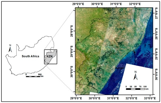
Figure 1.
KwaZulu-Natal province of South Africa with one of the Landsat ETM+ WELD composites (December 2011).
2.2. Existing Land Cover Maps for 2008 and 2011
Land cover maps used for training and validation were independently created by a consulting company for Ezemvelo KZN Wildlife using 20 m SPOT5 images acquired in 2008 [51] and 2011 [52]. Hereafter, for brevity, these are referred to as the EKZNW land cover maps. These maps were generated in support of a long term monitoring program designed to understand the impacts of land use and land cover change on biodiversity and ecological processes [50]. The classifications were derived using a combination of visual interpretation and classification techniques applied to single date SPOT 5 images. Some classes were compiled from ancillary data sets including the Eskom SPOT Building Count data, a map of Mangrove wetlands, and the National Field Crop Boundaries data set [52]. The land cover maps were defined with 47 land cover classes and were validated using approximately 1000 airborne observations with reported classification accuracies of 78% (2008) and 83.5% (2011) [50,52,53].
In this study, the EKZNW land cover maps were nearest neighbor resampled from 20 m to 30 m so that they could be compared to the 30 m Landsat data. The original 47 land cover classes were relabeled (“cross-walked”) to 22 aggregated classes (hereafter referred to as EKZNW classes) to provide a more reasonable goal for the automated the classification system. In addition, the 47 land cover classes were cross-walked to the 12-class scheme recommended by the Food and Agricultural Organisation’s (FAO) Land Cover Classification System 2 (LCCS2) that has been adopted by South Africa’s national mapping agency, National Geospatial Information (NGI) [54,55] (Appendix A). Our study therefore used the two levels of land cover class aggregation to test the ability of the LALCUM system to classify land cover at two levels of detail used at provincial (22 EKZNW classes) and national scales (12 NGI LCCS2 classes).
2.3. Landsat ETM+ Monthly WELD Composites
A total of 84 and 78 Landsat 7 Enhanced Thematic Mapper plus (ETM+) Level 1T images were obtained for the 12 calendar months of 2008 and 2011, respectively. The Landsat 7 ETM+ Level 1T data have six reflective wavelength bands, blue (band 1: 0.45–0.52 μm), green (band 2: 0.53–0.61 μm), red (band 3: 0.63–0.69 μm), near-infrared (band 4: 0.78–0.90 μm), short-wave infrared (band 5: 1.55–1.75 μm and band 7: 2.09–2.35 μm), and two thermal bands (band 6: both 10.40–12.50 μm with low and high gain settings). The WELD Version 1.5 processing algorithms [15] were used to generate 30 m monthly composited mosaics of KZN for 2011. The Version 1.5 WELD products store the six reflective top of atmosphere (TOA) Landsat 7 ETM+ bands, the two thermal bands and two cloud masks for each 30 m pixel [15]. The WELD products are defined in fixed geolocated tiles defined in the equal area sinusoidal projection. One of the major challenges faced by the LALCUM system was to produce useful land cover maps with the aid of WELD composites aimed at addressing the missing data caused the scan line corrector (SLC) failure of Landsat ETM+. Compositing procedures are applied independently on a per-pixel basis to the gridded WELD time series to reduce cloud and aerosol contamination, fill missing values due to the SLC failure (that removed about 22% of each Landsat ETM+ image [56]), and to reduce data volume. The WELD data have an established land cover mapping provenance and have been used, for example, to make land cover, land cover change, burned area, and field size maps at national scale [24,57,58,59].
2.4. Landsat-Derived Metrics for 2008 and 2011
The current state of the practice for large area multi-temporal land cover Landsat classification is to derive metrics from the satellite time series and then classify the metrics bands with a supervised non-parametric classifier [60]. The monthly WELD composites were processed to rank-based metrics which have been shown to provide a generalized feature space that has advantages over time-sequential composite imagery in mapping large area [28]. At each WELD pixel, the monthly composites were ranked according to their NDVI to capture phenological greenness. Since many of the pixels had no-data in several monthly composites, only the maximum, minimum and median NDVI-based ranks were used. The NDVI-based ranks (min., median, max.) were assigned to the corresponding Landsat derived metrics: TOA bands 1, 2, 3, 4, 5, and 7; NDVI; the two thermal bands; middle infrared/thermal infrared (MIRTIR); and to band ratios 3/5, 3/7, 4/5, 4/7, and 5/7.
2.5. Ancillary Data
A number of ancillary data sets were also used to improve the classification. The inclusion of static environmental features is common in regional land cover classification to help distinguish the same land cover type across different environments [61,62]. Maps of altitude, slope and aspect were derived from the ASTER Global Digital Elevation Model (ASTER GDEM) data (http://www.jspacesystems.or.jp/ersdac/GDEM/E/index.html). In addition, maps of mean annual precipitation (MAP) and mean annual temperature (Tmean) [63], were also included as they have been shown to provide class discriminative ability across large study areas. These data were resampled from 1.5 km to the WELD 30 m pixel grid.
3. Methods
3.1. Overview of Land Cover Mapping System
The Landsat Automated Land Cover Update Mapping (LALCUM) system is illustrated in Figure 2 and comprises the following functional five steps:
- The Iteratively Reweighted Multivariate Alteration Detection (IRMAD) change detection was applied to 2008 and 2011 image pairs to generate a spatially explicit 30 m 2008 to 2011 change mask. Function of Mask (FMASK) cloud detection was applied before the IRMAD change detection [64].
- Explanatory variables, i.e., monthly Landsat ETM+ WELD NDVI-ranked metrics (Section 2.4) (2011) and the ancillary data (Section 2.5), were prepared for all the study area at 30 m pixel resolution.
- Training data were derived by systematically sampling the 2008 EKZNW 30 m land cover map either with or without applying the 2008–2011 IRMAD change mask (Section 3.5. Classification experiments). The pixel samples were distributed systematically across the 2008 EKZNW 30 m land cover map following an area proportional allocation [65], but with additional allocation for very rare classes. At each selected pixel location a training sample defined by the 2008 EKZNW land cover class as the response variable, and the 2011 WELD and ancillary data as the explanatory variables, were extracted. The training data were independently derived in this manner ten times.
- The ten sets of training data were used to independently generate ten random forest (RF) models. The RF models were applied to every 30 m pixel of the 2011 explanatory variables to generate ten land cover maps for 2011. As there was very limited variability between the accuracies of the 10 RF models, one of the RF models were randomly chosen to produce the LALCUM map output for either 2008 or 2011.
- Independent validation of the classification accuracy of each of the ten 2011 land cover maps was undertaken by comparison with the pre-existing 2011 EKZNW land cover map, whilst excluding land cover polygons from which training data were extracted (Section 3.4.1 Accuracy Assessment—Map comparison).
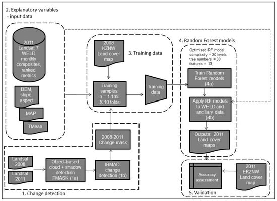
Figure 2.
Overview of the Landsat Automated Land Cover Update Mapping (LALCUM) system. The dashed polygons indicate the components responsible for five steps of the process.
The processing time of the system components were evaluated and reported below.
3.2. 2008 to 2011 Change Detection and Validation
The Iteratively Reweighted Multivariate Alteration Detection (IRMAD) approach was selected for image pair normalization and change detection. The Multivariate Alteration Detection (MAD) algorithm is based on the assumption that the satellite pixel values (in all spectral bands) of one image can be related to the co-registered pixels in a second image by a linear transformation (determined using Canonical Correlation Analysis). This, to first-order, reduces atmospheric differences and small phenological differences. The IRMAD algorithm extends this model, allowing some pixels to be systematically excluded from the calculation of the MAD linear transformation and thus using only unchanged pixels in the calculation [47,48]. The MAD variates produced by the IRMAD algorithm have approximately a multivariate Gaussian distribution [47]. The Chi-square statistic computed from the MAD variates can be thresholded to identify outliers, which are changed pixels. Nielsen and Canty used the 99.9th percentile of the chi-squared statistic over all pixels as the threshold [47]. Initial evaluation of this approach over the study area was unsatisfactory, and a different approach was adopted. The asymmetry in the distribution of the per-pixel chi-squared values was isolated, and subsequently used to evaluate a minimum-error Bayes discriminant, yielding thresholds between the 90th and 93rd percentile across the 2008-to-2011 image pairs covering the study area.
Near-cloud free Landsat L1T images were selected for near anniversary dates in the autumn of 2008 and 2011 to reduce phenological differences. Cloud and cloud shadows were identified using the FMASK algorithm [64] and excluded as they could bias global image statistics and the IRMAD change detection process. IRMAD was applied to the resulting pairs of 2008 and 2011 and not to the monthly WELD composites. Multi-date composites are not suitable as input to the basic IRMAD algorithm, since only a single linear transformation is calculated per composite pair, which would not accommodate all the potential date combinations present in the composites. Although several forest monitoring systems perform change detection based on annual rank-based metrics [28,58] and it would have simplified the LALCUM system, we expected that the multiple forms of land cover change which need to be detected in our study area would require a more sensitive spectral change detection method. Since almost 22% of each of the bi-temporal Landsat ETM+ image is lost due to the SLC-off error, change detection could only be effectively applied across about 66% of the study area. Areas where the change status could not be discerned due to the SLC-off error were therefore ignored. The resulting 30 m 2008 to 2011 change mask was defined for each pair of L1T images and clusters of change pixels larger than 3 ha were vectorized to polygons of change.
Validation can be conducted using individual pixels, blocks of pixels or polygons as units of assessment, each with their own set of advantages and disadvantages [66]. In our experience, operators found it hard to visually interpret individual pixels and were actually judging the change in context of a much larger cluster of pixels, making a polygon-based validation more appropriate for evaluating the general utility of a change mask over our large diverse study area. The change polygons were validated using an on-line validation system developed for this task that enabled visual comparison with SPOT 2.5 m pan-sharpened true color images of 2008 and 2011 (provided by South African National Space Agency—SANSA, as a Web Map Service), overlaid with the IRMAD change polygons. There was a very high abundance of change polygons smaller than 5 ha. Therefore, in order to ensure a greater representation, polygons were binned into the following size classes and sampled equally: 3–5, 5–10, 10–15, 15–30, 30–50, and 50–500 ha. The system enabled the operator to rapidly, visually assess and record land cover changes with a bounding box (and at three zoom levels) around each automatically selected IRMAD change polygon. The operator judged the label of the polygon (change or no-change) based on a majority rule, i.e., if more than 50% of a polygon changed, it was considered correct, but if less than 50% changed, it was considered a false detection [66]. Pixel-level errors along the edges of change polygons were ignored as these were largely due to the mismatch in image resolution (30 m Landsat vs. 2.5 m SPOT). To evaluate the ability of IRMAD to identify no-change areas, no-change polygons were also simulated and included in the evaluation set (25% of total number of polygons) by randomly relocating actual change polygons, whilst avoiding potential change areas. Change detection was only validated in areas not affected by the SLC error in either of the 2008 or 2011 images in a pair. A total of 1547 polygons larger than 3 ha were validated by one of five operators.
3.3. Random Forest Implementation
The Random Forest (RF) classifier was used as it is an established supervised non-parametric classifier that can accommodate nonlinear relationships between variables and makes no assumptions concerning their statistical distributions [67]. This is particularly important given the different kinds of explanatory variables used. RF supervised classifiers create an ensemble of decision tree classifications on different training data subsets and decides how to classify each pixel based on the mode class labels assigned by all the decision trees [67]. The random forest classifier provides reduced likelihood of over-fitting explanatory variables to the training data by independently fitting a large number of decision trees, with each tree grown using a random subset of the training data and a limited number of randomly selected predictor variables [67].
The Waikato Environment for Knowledge Analysis (WEKA) implementation of RF was used in this study [68] (Step 4, Figure 2). Constraining the RF complexity allows comparable classification accuracies to be achieved with significantly simpler RF models, which is required to reduce the computational load when classifying large data sets [61]. The WEKA RF enables the following constraining parameters: (a) the number of decision trees per RF model; (b) the maximum decision tree depth; and (c) the number of attributes (randomly selected at training time) made available to each decision tree. A systematic grid search was employed to identify a combination of constraining parameters that offered a good trade-off between model complexity, and training validation performance. In this study area, a combination of 20 attributes (out of a possible 57) per decision tree, with a maximum tree depth of 18 levels and a total of 30 decision trees per RF model was found to provide good balance between accuracy and complexity to ensure operational feasibility. We therefore refrained from using 500 trees which is most commonly used because it is the default in the R statistical package [62].
3.4. Classification Accuracy Assessment
3.4.1. Map Comparison
The LALCUM system produced a complete land cover map for each of the 10 folds of the four treatments and classification accuracy was assessed across the entire study area by comparing each pixel in the validation set (n = 9,316,862) to the corresponding land cover label in the 2011 EKZNW map. This design allowed all pixels in the map to be evaluated objectively, with no spatial overlap between regions (polygons) used for training and regions used for validation. The validation data from the reference map were used to generate a two-way confusion matrix (Step 5, Figure 2). Conventional accuracy statistics (kappa, user’s and producer’s accuracy) were then derived from the confusion matrix [69]. For brevity, only the overall, user’s and producer’s accuracies were reported. The producer’s accuracy (PA) relates to how well a certain area can be classified and was calculated as the number of pixels of the EKZNW reference map (validation data) in a particular land cover class which have been correctly classified by the LALCUM system. The producer’s accuracy is the inverse of omission error (omission error = 1 − producer’s accuracy) i.e., how often areas of a particular land cover in the EKZNW reference map were not classified as belonging to that land cover class by the LALCUM system. The user’s accuracy (UA) is indicative of the probability that a pixel classified as belonging to a particular land cover class in the LALCUM-derived map actually belonged to that land cover class according to the EKZNW reference map (validation data) [66]. User’s accuracy is the inverse of commission error (commission error = 1 − user’s accuracy), i.e., how often areas included as a particular class in the LALCUM map, actually belonged to a different class.
3.4.2. Airborne Validation
An airborne survey was undertaken by EKZNW in 2011 to capture a series of oblique aerial photographs (1715) for assessing the accuracy of the land cover maps [53]. A set of validation points (985) were created from the original set after interpreting the aerial photographs and SPOT imagery and relocating the point in the location of the land cover type instead of the GPS location of the aircraft [52]. The airborne validation points were used as the reference data to calculate accuracies described above (Section 3.4.1).
3.5. Classification Experiments
The LALCUM system was used to conduct experiments at operational scales to determine the classification accuracy of various approaches using the above-mentioned map comparison and airborne validation. The main experiment tested how the difference in accuracy achieved with and without applying the change mask (Step 1, Figure 2) to the training data (Step 3, Figure 2). More specifically, the experiments were set up to test how accurately the LALCUM system could create a land cover map of the KwaZulu-Natal Province for 2011 using training data from the 2008 land cover map after applying a change detection mask (2008–2011) (treatment 3 below), compared to using no change mask (treatment 4 below). In addition to the aforementioned treatments, two controls were applied. The four treatments were:
- Generate 2008 land cover with 2008 Landsat images and 2008 land cover labels (control).
- Generate 2011 land cover with 2011 Landsat images and 2011 land cover labels (control).
- Generate 2011 land cover with 2011 Landsat images and 2008 land cover labels after applying a 2008–2011 change mask. The system configuration for treatment 3 is given in Figure 2.
- Generate 2011 land cover with 2011 Landsat images and 2008 land cover labels with no change mask applied (excluding Step 1, Figure 2).
4. Results
4.1. Change Detection Validation
A total of 1997 change polygons were visually inspected by one of five operators. Approximately 11% of the change detected by IRMAD was due to remnant cloud and cloud shadow not detected by FMASK, while another 5% of change detected was due to unseasonal early burned area in grasslands and wetlands. After omitting the afore-mentioned instances of clouds or burns from the data, 16.5% of the change detected by IRMAD was not deemed to be true land cover change by the operator (false positives) (Table 1). The change detection accuracy was 83.5%, i.e., the change detected was considered to be true change (true positive). Approximately 93% of the simulated polygons containing no change, were identified as such by the operator (true negative). This is in agreement with the empirically determined threshold value (Methods Section), which implied a false negative detection rate of 7%.

Table 1.
Visual validation of change detection polygons following removal of erroneous cloud and burned area detections.
Most of the change detected was dominated by two forms of change: (i) 35% of all changes were caused by clear felling of commercial, exotic forestry plantations and their regrowth; and (ii) 56% of all changes were within cultivated fields including changes from active dryland, irrigated, sugarcane to bare soil or fallow fields. Together, the changes in forestry plantations and cultivation accounted for 91% of detected change after excluding erroneous changes due to clouds or burned area.
The IRMAD change mask was also compared to a change mask derived from 2008 vs. 2011 EKZNW land cover maps. The two masks agreed that approximately 7%–8% of the study area had changed, however there was only a 21.3% agreement between the IRMAD and EKZNW change masks. The classes which change the most relative to their 2008 labels according to EKZNW maps were “Plantations—clearfelled”, “Cultivation commercial annual crops dryland”, “Mines and Quarries”, and “Degraded Forest, Bushland and old fields”.
4.2. Accuracy Assessment—Map Comparison
There was very low variability in the overall accuracy (SD < 1.4%) between the ten folds of each treatment (Table 2), indicating that the generation of different sets of training samples did not cause variability in the classification accuracy. The 2008 land cover created using the 2008 labels (treatment 1) had the highest accuracy in both the 22- and 12-class cases of 67.3% and 73.9%, respectively. The 2011 land cover created using the 2011 labels (treatment 2) had an accuracy of 65.9% and 73.4% for 22 and 12 classes, respectively. In all the treatments, the 12-class NGI-LCCS case had approximately 6% higher accuracy than the 22-class EKZNW case due to the aggregation of classes.
Table 2.
Overall accuracy of land cover classification treatments with standard deviation (SD) of accuracy across the ten repetitions (folds) in parentheses for the EKZNW and NGI-LCCS land cover classes.
For the 22 EKZNW classes, the application of the IRMAD change mask did not increase the accuracy when generating a 2011 land cover using 2008 land cover labels and both treatment 3 and 4 had an accuracy of approximately 65% (Table 2). Using the 2008 labels and no change mask (treatment 4) to produce the 2011 land cover only had a 1% lower accuracy than when using the 2011 labels (treatment 2). When using the 12 NGI-LSSC classes, the application of IRMAD change mask had little effect (treatments 3 and 4), while the use of the 2011 labels (treatment 2) vs. the 2008 labels (treatment 4) had 1.3% higher accuracy (Table 2).
When comparing the PA of individual classes between treatments, the “Plantations—clearfelled” class, which is a rapidly changing class, had an accuracy of only 15% in treatment 4 (2008 labels, no change mask), but this increased to 62% when the IRMAD mask and 2008 labels were used (treatment 3). Otherwise there were no notable differences in the per-class accuracy that could be attributed to the application of the change mask. Therefore only the per-class accuracies of treatment 2 will be reported below.
The LALCUM system produced land cover maps with coherent distributions of land cover classes that had a general good agreement with the EKZNW maps (Figure 3, Figure 4 and Figure 5). The missing data caused by scan line corrector failure of Landsat ETM+ was not evident in the LALCUM produced land cover maps. In the area of the Lake St. Lucia (iSimangaliso Wetland Park—World Heritage site) the main land cover classes (“Water”, “Wetlands”, “Forests (indigenous)”, “Plantations”, “Sugarcane”, “Plantations”, Plantations clearfelled, Built up/Dense settlement, Subsistence Cultivation) were very accurately mapped by the LALCUM system while “Degraded Forest, Bushland and old fields (previously bushland)” was confused with “Medium bush (<70% cc)” (Figure 3). In the area around the town of Greytown, the main land cover classes (“Wetlands”, “Plantations”, “Sugarcane”, “Plantations”, “Plantations—clearfelled”, “Built up/dense settlement”, and “Subsistence Cultivation”) appear to be accurately mapped although the exact boundaries differed (Figure 4).
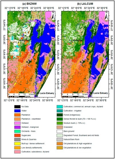
Figure 3.
EKZNW land cover map for area surrounding Lake St. Lucia, iSimangaliso Wetland Park—World Heritage site, 2011 (a) and the land cover produced by the LALCUM system (b).
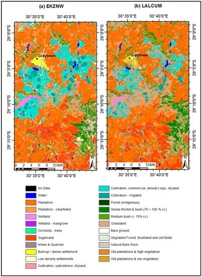
Figure 4.
EKZNW land cover map for area surrounding Greytown, 2011 (a) and land cover produced by the LALCUM system (b).
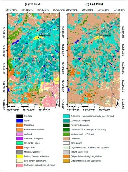
Figure 5.
EKZNW land cover map for area surrounding Winterton, 2011 (a) and land cover produced by the LALCUM system (b).
The UA and PA were calculated for each land cover class for treatment 2 (Table 3). The percentage contribution to overall error was also calculated from the counts of incorrectly classified validation pixels as a percentage of the total incorrect pixels, thus taking into account the total area covered by a class (Table 3). “Water”, “Plantations”, “Plantations—clearfelled”, “Orchards—trees”, “Sugarcane”, “Built-up/dense settlement”, “Cultivation—Irrigated” and “Forest (indigenous)” had UA above 70% (commission errors < 30%) and there was a relatively good agreement between the EKZNW and LALCUM maps for these classes (Figure 3 and Figure 4). However, apart from “Water”, “Plantations” and “Sugarcane”, which had PA above 70%, most of the afore-mentioned classes had much lower PAs (omission errors > 45%), indicating that they were underestimated. The opposite was however true for the natural vegetation classes “Grasslands”, “Medium Bush” and “Dense Thicket and Bush”, which had a higher PA than UA, i.e., higher commission error than omission error, which indicates that these classes were overestimated by the LALCUM system. Together these three natural vegetation classes accounted for 35.7% of the overall error (Table 3).
Table 3.
Accuracy of each of the EKZNW land cover classes and their percentage contribution to overall error in 2011 LALCUM produced land cover map, based on the map-to-map accuracy assessment (Treatment 2).
The “Degraded Forest, bushland and old fields” class was spectrally indistinguishable from most of the afore-mentioned classes and had a PA and UA of only 2.9% and 28.5%, respectively. The class “Cultivation subsistence dryland”, covers large areas and had a low UA of 48.6% and PA of 18.6% which was the single largest contributor to overall error (18%) (Table 3). Subsistence cultivation is a notoriously difficult class to map in South Africa [70,71] as only approximately 14% of subsistence fields are cultivated in any given year and the fallow fields are spectrally indistinguishable from areas of low grass cover within the “Grasslands” and “Bare ground” classes (Figure 5). As a result, large areas of “Cultivation subsistence dryland” were mapped as “Grasslands” (Figure 5). Similarly, “Low density settlements” had a low PA of 15.6% and UA of 36.8%, contributing 8% to overall error. This class consists of small dwellings in rural areas interspersed by mostly fallow fields of subsistence cultivation and natural vegetation that are spectrally indistinguishable from “Grasslands”, “Medium bush”, and “Cultivation subsistence dryland” (Figure 6).
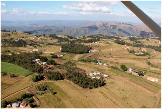
Figure 6.
Oblique photograph taken during airborne validation illustrating the complex mosaic of low density, small dwellings within the “Low density settlements” land cover class, interspersed by small fields of active and fallow “Cultivation subsistence drylands”, as well as “Plantations”. (Photo credit: John Craige, Ezemvelo KZN Wildlife).
The class “Cultivation, commercial, annual crops, dryland” had a low PA of 28% and UA of 63.8% (Table 3). This was due to the fact that the EKZNW land cover map included both active and fallow fields from the manually digitized National Field Crop Boundaries data set, while the LALCUM system only classified actively cultivated fields in this class. This led to high apparent omission errors as fallow fields were mapped as “Bare ground” or “Grasslands” (Figure 4 and Figure 5), while the commission errors were more acceptable due to the classifier’s ability to identify active cultivation. The “Cultivation—irrigated” class appeared to suffer from the same afore-mentioned problem with a PA of 41.9%, but a high UA of 70.9% (Table 3) (Figure 4 and Figure 5). Since the LALCUM system uses an annual time series of Landsat ETM+ images it is unlikely that the imagery would not have capture the growing period of crops in the actively cultivated fields. The accuracy with which the LALCUM system was mapping active cultivation (commercial, annual crops dryland and irrigated) was therefore most likely underestimated by comparing it to EKZNW maps, which included fallow fields.
The aggregation of the 22 EKZNW classes into the 14 NGI-LCCS classes had a positive influence on most of the per-class accuracies (Table 4, Appendix A). By combining all the cultivation (irrigated, dryland, commercial and subsistence and sugarcane) into one LCCS class, i.e., “Cultivated and Managed Terrestrial Primary Vegetated Areas Herbaceous Graminoids”, resulted in a higher per-class UA of 81.5%, compared to the low UAs of 63.4%, 48.6% and 70.9% respectively achieved for “Cultivation commercial, annual crops, dryland”, “Cultivation subsistence, dryland” and “Cultivation—irrigated” (Table 3 and Table 4 and Appendix A). Combining “Dense thicket and bush”, “Medium bush”, as well as “Degraded Forest, Bushlands and old fields” into one NGI-LCCS class named “Natural and Semi-Natural Terrestrial Primary Vegetated Areas: Shrubs and Bushes” resulted in much higher UA and PA of 75.6% and 76.4%, respectively. The “Grasslands” class, which was now called “Natural and Semi-Natural Terrestrial Primary Vegetated Areas: Graminoids”, displayed the same overestimation indicated by the higher PA (88.8%) and lower UA (68.2%) as discussed above for the 22 EKZNW classes (Table 3 and Table 4).
Table 4.
Accuracy of each of the NGI-LCCS classes in 2011 KwaZulu-Natal land cover map (Treatment 2).
4.3. Accuracy Assessment—Airborne Validation
The airborne surveys estimated the overall accuracy of the 2011 EKZNW land cover map (resampled to 30 m resolution) aggregated to 22 EKZNW classes, at 83%, while the highest overall accuracy of the map produced by the LALCUM system was only 58% (treatment 2). The LALCUM system mapped “Water”, “Plantations”, “Sugarcane”, “Grasslands”, “Bare ground”, “Dense Thicket and Bush” with PA above 70%, while “Built-up dense settlements” had a PA of 68% (Table 5). The low overall accuracy of 58% was largely due to a number of ambiguous classes which could not be distinguished spectrally, namely “Plantation—clearfelled”, “Degraded Forest, Bushland and old fields”, “Cultivation subsistence dryland”, “Wetland—mangrove”, “Old plantations and high vegetation”. In agreement with the map comparisons above, the natural vegetation classes “Grasslands”, “Medium Bush” and “Dense Thicket and Bush”, which had a higher PA than UA, which indicates that these classes were overestimated by the LALCUM system. Using the 12 NGI-LCCS classes overall accuracy of LALCUM system and the EKZNW maps were 66% and 87% respectively (treatment 2). The per-class accuracies for the 22 EKZNW classes vs. the 12 NGI-LCCS classes showed similar trends for the airborne validation compared to the map comparison discussed above.
Table 5.
Accuracy of each of the EKZNW land cover classes and their percentage contribution to overall error in 2011 KwaZulu-Natal land cover map, based on airborne validation data (Treatment 2).
4.4. System Processing Time Evaluation
The processing time of each of the system components or functional steps (Section 3.1 and Figure 2) were evaluated (Table 6). The processing system comprised of a dual-socket Xeon E5-2680 with a total of 16 cores operating at 2.7 GHz and 256 GB of RAM. The slowest part of the system was the FMASK cloud detection which was not an optimized C++ implementation and can be improved in future. The entire system was run in 9.5 h, thus allowing rapid land cover map updates. Once component 1 (cloud and change detection) was completed, any one of the four treatments (components 2–5) could be run in 5.2 h, thus enabling experimentation at operational scales.
Table 6.
Processing time (minutes) of LALCUM system components or functional steps outlined in Section 3.1 and Figure 2.
5. Discussion
The objective of the study was to develop a system capable of rapidly updating a land cover map from a reference year to a subsequent desired year. Our strategy was to automatically create a very large volume of training samples (n > 1 million) using the existing EKZNW map (2008) as land cover labels and train an optimized, robust RF classifier to rapidly classify land cover for a desired year (2011) across a large, heterogeneous study area. In an attempt to improve the accuracy of the RF classifier we applied a change detection algorithm to identify and excluded training samples which may have experienced land cover change between the date of the initial reference land cover map (2008) and the later desired date (2011), as these samples would be mislabeled and were expected to lead to classification errors and reduced accuracy.
In keeping with the principle of parsimony, the RF parameters were optimized to achieve a balance between model complexity (size of the RF classifier) and classifier generalization performance [61]. The Weka RF implementation initially exhibited signs of overfitting (here taken to mean a large difference between training and validation error) if no constraints were placed on RF complexity. Limiting the number of trees, as well as the maximum depth per tree, was found to reduce model complexity and close the gap between training and validation error. Reducing the number of trees (from 100 to 30) incurred a loss of about 2% in validation accuracy, which was recovered by increasing the number of attributes allocated per tree from 6 to 20.
The overall agreement between land cover maps generated by the LALCUM system and the EKZNW maps was assessed at more than nine million points. The 2008 land cover created using the 2008 labels (treatment 1) had the highest overall accuracy in both the 22- and 12-class cases of 67.3% and 73.9%, respectively (Table 2). The 2011 land cover created using the 2011 labels (treatment 2) had an overall accuracy of 65.9% and 73.4% for the 22 and 12 classes, respectively. These accuracies were similar to those achieved by the MAD-MEX system in Mexico for 10–13 classes, i.e., 62%–66% [6]. The US NLCD achieved an overall user accuracy of 78% at LevelII with 16 classes, which is an impressive accuracy at national scale [72]. In all treatments, the 12-class NGI-LCCS case had approximately 6% higher accuracy than the 22-class EKZNW case, due to the aggregation of spectrally similar classes.
The natural vegetation classes “Grasslands”, “Medium Bush” and “Dense Thicket and Bush”, which had a higher PA than UA, i.e., higher commission error than omission error, which indicates that these classes were overestimated by the LALCUM system (Table 3). This was mainly due to the area proportional allocation of training samples [57] to these three very large natural vegetation classes and the objective of the RF classifier to maximize overall accuracy, often at the expense of the smaller individual classes. As a result, smaller classes such as “Forest (indigenous)” and “Natural Bare Rock” were underestimated and have much higher UA than PA, i.e., lower commission errors than omission errors (Table 3). The EKZNW maps included both active and fallow fields mapped visually as part of the National Field Crop Boundaries data set, while the LALCUM system only classified areas of actively growing crops in the class “Cultivation, commercial, annual crops, dryland” (Figure 5), contributing to a low PA (28%) and 8.7% contribution to overall error (Table 3). Although a number of land cover classes could be distinguished by their spectral properties (e.g., “Plantations”, “Water”, “Sugarcane” and “Grasslands”), other classes could not. The latter classes (e.g., “Cultivation, subsistence, dryland”, “Low density settlements”, “Degraded Forest, Bushland and old fields”) were originally mapped through visual interpretation of pan-sharpened SPOT5 imagery and ancillary data sets which focused on mapping individual classes (e.g., “Wetlands”, “Wetlands Mangroves”, “Orchards Trees”) [52]. This visual interpretation took the shape, pattern and spatial context of high resolution features into account. The results suggest that these detailed classes, which are required for operational, provincial-scale land use planning, can therefore, not be mapped using Landsat spectral data alone. On the other hand, when the LALCUM system was applied using the 12 aggregated NGI-LCCS classes, it achieved higher levels of accuracy (up to 74%), which are useful at national scales for monitoring and reporting, e.g., land cover maps used as inputs to national greenhouse gas emissions inventory [2]. The study therefore indicates a very clear limit in the accuracy of automated land cover classification based solely on spectral information in the context of operational user requirements for detailed land cover information containing classes which are routinely mapped using visual interpretation.
According to our visual change detection validation the IRMAD change detection was 83% accurate with 7% false detection rate. Ninety-one percent of all of the change detected was either within cultivated fields or commercial forestry plantations which change very rapidly without constituting major changes in land use. These two forms of land cover change are not only the most abundant, but also spectrally the most pronounced forms of change which can obfuscate more subtle, but important changes (e.g., the expansions of human settlements), when using a single change metric threshold per image pair. An alternative approach would be setting a different change threshold for different land cover classes based on the per-class distribution of the change metric values [11]. Change detection methods are also evolving from the image pair approaches to continuous time-series analyses of spectral change in medium to high resolution imagery [22,23,26,27,36,73]. Such continuous monitoring can provide information on persistence and direction of change in the context of natural seasonal variability and may provide continuous near-real time land cover change alerting in the near future [27].
In line with the approach proposed by U.S. Geological Survey [11,46], we hypothesized that applying change detection before training a random forest classifier using only non-change samples would increase the accuracy of the classification as it would decrease mislabeled sampled in the training set. However, according to our results, the application of the change mask did not increase the accuracy and both treatments 3 and 4 had an accuracy of 65%. Using the 2008 labels and no change mask (treatment 4) to produce the 2011 land cover only have a 1% lower accuracy than using the 2011 labels. Since only 7.5% of the study area changed between 2008 and 2011 resulting in approximately 7.5% mislabeled data, this was not enough to reduce the accuracy of the RF classifier. In other studies it was established that mislabeling of more than 20% of the training data resulted in an exponential increase in error [61]. To further explore the robustness of our RF classifier to noise, we simulated 5%–70% mislabeled training data and tracked the resulting reduction in overall classification accuracy (producer accuracy, map-to-map) (Figure 7). Taking into account that the training data derived from EKZNW maps already include 20% mislabeled samples due to the error of the maps (accuracy of 80%) [51,52], this initial 20% was added to the simulated percentage of mislabeling (Figure 7). Even though the robustness of RF classifiers to mislabeling is well documented [61,62,67,74] it was not expected to tolerate up to 50% mislabeling before the overall accuracy reduced below 60%. The inherent robustness of the RF was potentially enhanced by the very large number of training sampled used (n > 1 million). Due to the RF’s robustness to mislabeling and the relatively low levels of change (7.5% between 2008 and 2011), the change detection step to mask out changed samples did not yield any benefits. However, where levels of change reach above 20%–30% in a particular region, the change detection step can only enhance RF classification accuracy. Therefore, although applying a change mask to omit incorrect data labels before training a classifier should logically hold benefits [11], it did not improve the overall accuracy in our study period and study area. The only benefit of applying the change mask was an improvement in the accuracy of one class rapidly changing class namely “Plantations—clearfelled”, from 15% in treatment 4 (2008 labels, no change mask), to 62% (IRMAD mask and 2008 labels) (treatment 3). We therefore urge developers of similar land cover mapping systems to test the benefits of a change detection step for their own circumstances.
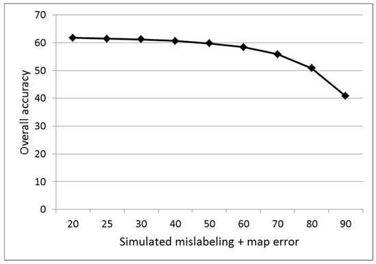
Figure 7.
Overall accuracy of Random Forest classification after simulating additional mislabeled training samples in addition to the 20% error contained in the original EKZNW land cover maps on which it was trained.
The approach and the LALCUM system may be improved by using Landsat 8 due to its greater 12-bit quantization (compared to Landsat ETM+ 8-bit) and improved signal-to-noise characteristics, as well as the absence of the SLC error and more frequent, global data acquisition [12], all of which could contribute to enhanced spectral discrimination between some of the problematic land cover classes. The inclusion of Synthetic Aperture Radar (SAR) data as additional explanatory variables which are sensitive to woody vegetation structure (cover height and biomass) [75,76] may improve the discrimination between the natural vegetation classes “Grasslands”, “Medium Bush”, “Dense Thicket and Bush” and “Forest (indigenous)” which made a significant contribution to overall error. Optical and SAR data are increasingly being combined as complementary features in land cover change detection and mapping systems with enhanced results [38,77]. The IRMAD change detection component of the LALCUM, which was applied to single image pairs, can be improved by using change detection methods that analyze the complete time series on a continuous basis [22,35,77]. Most of the aforementioned improvements to the LALCUM system are being implemented.
6. Conclusions
The approach of automatically creating very large amounts of training labels from an existing land cover map and using a robust RF to classify land cover from Landsat imagery for a subsequent desired year proved to be feasible for rapidly updating land cover maps provided that the land cover classes are spectrally separable at a useful level of thematic aggregation. Following the WELD preprocessing, the entire system was run in 9.5 h, thus allowing rapid land cover map updates and experimentation at operational scales. The application of a change mask to exclude training samples where land cover changed between the reference year and the desired year did not increase the classification accuracy due to the robustness of Random Forest classifier to mislabeled training samples. This robustness to potential mislabeling caused by land cover change, suggests that a random forest classifier can be trained using a reference land cover map even if there has been a 10%–20% change in land cover. However, in areas with more rapid land cover change the application of the change mask before training the classifiers may improve the classification accuracy. With the increase in free and frequent medium to high resolution satellite data, such as Landsat 8 and Sentinel 2, and rapid growth of local and cloud-based computing capacity, we expect a proliferation in “locally-tuned” land cover products with higher operational utility than currently available global or continental land cover products [16]. Frequently updated land cover data will continue to be in high demand as competing land uses transform land, often at the expense of ecosystem services and long-term human well-being.
Acknowledgments
The research was partially funded by the CSIR and the Department Rural Development and Land Reform, National Geo-spatial Information (NGI). We are especially grateful to Aslam Parker of NGI for his support. Ezemvelo KZN Wildlife and GeoTerraImage provided access to land cover data and airborne validation data. Land cover data sets: Ezemvelo KZN Wildlife; KwaZulu-Natal land cover 2011 v1 (clp_KZN_2011_LC_v1_grid_w31.zip) (GIS coverage); Pietermaritzburg: Biodiversity Research and Assessment, Ezemvelo KZN Wildlife, 2013, Ezemvelo KZN Wildlife; KwaZulu-Natal land cover 2008 v2 (clp_KZN_2008_LC_v2_grid_w31.zip) (GIS coverage); and Pietermaritzburg: Biodiversity Research and Assessment, Ezemvelo KZN Wildlife, 2013.
Author Contributions
K.J.W., F.v.d.B., B.M. and B.P.S. conceived and designed the experiments; F.v.d.B., B.M., and~B.P.S. performed the experiments; D.S., K.C.S., B.P.S., and B.M. processed and analyzed the data; B.M., D.S. and K.C.S. contributed materials/analysis tools; and K.J.W., F.v.d.B., D.P.R., D.J. and K.C.S. wrote the paper.
Conflicts of Interest
The authors declare no conflict of interest.
Appendix A
Table A1.
The aggregated Ezemvelo KZN Wildlife (EKZNW) land cover classes (22) cross-walked to Food and Agricultural Organisation’s (FAO) Land Cover Classification System 2 (LCCS2) used by South Africa’s national mapping agency, National Geospatial Information (NGI) (12 classes).
| EKZNW Aggregated Land Cover Class Names | NGI-LCCS Level 1 Class Name | LCCS Level 2 Class Name |
|---|---|---|
| Water | Natural Non-Vegetated Aquatic or Regularly Flooded Water Bodies | water |
| Plantation | Cultivated and Managed Terrestrial Primary Vegetated Areas | Needle leaved (default) |
| Plantation—clearfelled | Cultivated and Managed Terrestrial Primary Vegetated Areas | Broad Leaved Bushes and Shrubs |
| Wetland | Natural or Semi-Natural Aquatic or Regularly Flooded Vegetated Areas | Herbaceous |
| Wetland—mangrove | Natural or Semi-Natural Aquatic or Regularly Flooded Vegetated Areas | Woody Wetlands |
| Orchards—trees | Cultivated and Managed Terrestrial Primary Vegetated Areas | Broad leaved evergreen (default) |
| Sugarcane | Cultivated and Managed Terrestrial Primary Vegetated Areas | Herbaceous Graminoids |
| Mines and Quarries | Artificial Terrestrial Primarily Non-Vegetated Areas | Non-Built-up Artificial Bare Area |
| Built-up/dense settlement | Artificial Terrestrial Primarily Non-Vegetated Areas | Built-up Urban/Residential Areas |
| Low density settlements | Artificial Terrestrial Primarily Non-Vegetated Areas | Built-up Urban/Residential Areas |
| Cultivation, subsistence, dryland | Cultivated and Managed Terrestrial Primary Vegetated Areas | Herbaceous Graminoids (default) |
| Cultivation, commercial, annual crops, dryland | Cultivated and Managed Terrestrial Primary Vegetated Areas | Herbaceous Graminoids (default) |
| Cultivation—irrigated | Cultivated and Managed Terrestrial Primary Vegetated Areas | Herbaceous Graminoids (default) |
| Forest (indigenous) | Natural and Semi-Natural Terrestrial Primary Vegetated Areas | Trees |
| Dense thicket and bush (70% > 100% cc) | Natural and Semi-Natural Terrestrial Primary Vegetated Areas | Shrubs and Bushes |
| Medium bush (<70% cc) | Natural and Semi-Natural Terrestrial Primary Vegetated Areas | Shrubs and Bushes |
| Bush Clumps/Grassland | Natural and Semi-Natural Terrestrial Primary Vegetated Areas | Shrubs and Bushes |
| Grassland | Natural and Semi-Natural Terrestrial Primary Vegetated Areas | Graminoids |
| Bare ground | Natural Terrestrial Non-Vegetated Bare Areas | Unconsolidated Bare Soil |
| Degraded Forest, Bushland and old fields (previously bushland) | Natural and Semi-Natural Terrestrial Primary Vegetated Areas | Shrubs and Bushes |
| Natural Bare Rock | Natural Terrestrial Non-Vegetated Bare Areas | Consolidated Bare Rock and Coarse Fragments |
| Old plantations and high vegetation | Cultivated and Managed Terrestrial Primary Vegetated Areas | Broad Leaved Bushes and Shrubs |
| Old plantations and low vegetation | Cultivated and Managed Terrestrial Primary Vegetated Areas | Broad Leaved Bushes and Shrubs |
References
- DeFries, R.S.; Foley, J.A.; Asner, G.P. Land-use choices: Balancing human needs and ecosystem function. Front. Ecol. Environ. 2004, 2, 249–257. [Google Scholar] [CrossRef]
- Verburg, P.H.; Neumann, K.; Nol, L. Challenges in using land use and land cover data for global change studies. Glob. Chang. Biol. 2011, 17, 974–989. [Google Scholar] [CrossRef]
- Foley, J.A.; DeFries, R.; Asner, G.P.; Barford, C.; Bonan, G.; Carpenter, S.R.; Chapin, F.S.; Coe, M.T.; Daily, G.C.; Gibbs, H.K.; et al. Global consequences of land use. Science 2005, 309, 570–574. [Google Scholar] [CrossRef] [PubMed]
- Hansen, M.C.; Loveland, T.R. A review of large area monitoring of land cover change using Landsat data. Remote Sens. Environ. 2012, 122, 66–74. [Google Scholar] [CrossRef]
- Burkhard, B.; Kroll, F.; Nedkov, S.; Muller, F. Mapping ecosystem service supply, demand and budgets. Ecol. Indic. 2012, 21, 17–29. [Google Scholar] [CrossRef]
- Gebhardt, S.; Wehrmann, T.; Ruiz, M.; Maeda, P.; Bishop, J.; Schramm, M.; Kopeinig, R.; Cartus, O.; Kellndorfer, J.; Ressl, R.; et al. Mad-Mex: Automatic wall-to-wall land cover monitoring for the Mexican REDD-MRV program using all Landsat data. Remote Sens. 2014, 6, 3923–3943. [Google Scholar] [CrossRef]
- Fry, J.A.; Xian, G.; Jin, S.M.; Dewitz, J.A.; Homer, C.G.; Yang, L.M.; Barnes, C.A.; Herold, N.D.; Wickham, J.D. National land cover database for the conterminous United States. Photogramm. Eng. Remote Sens. 2011, 77, 859–864. [Google Scholar]
- Wessels, K.J.; Reyers, B.; van Jaarsveld, A.S.; Rutherford, M.C. Identification of potential conflict areas between land transformation and biodiversity conservation in north-eastern South Africa. Agric. Ecosyst. Environ. 2003, 95, 157–178. [Google Scholar] [CrossRef]
- GeoTerraImage. 2013–2014 South African National Land-Cover Dataset: Data User Report and Metadata; GeoTerraImage (South Africa): Pretoria, South Africa, 2015; pp. 1–53. [Google Scholar]
- Fairbanks, D.H.K.; Thompson, M.W.; Vink, D.E.; Newby, T.S.; Van den Berg, H.M.; Everard, D.A. The South African land-cover characteristics database: A synopsis of the landscape. S. Afr. J. Sci. 2000, 96, 69–82. [Google Scholar]
- Xian, G.; Homer, C.; Fry, J. Updating the 2001 national land cover database land cover classification to 2006 by using Landsat imagery change detection methods. Remote Sens. Environ. 2009, 113, 1133–1147. [Google Scholar] [CrossRef]
- Roy, D.P.; Wulder, M.A.; Loveland, T.R.; Woodcock, C.E.; Allen, R.G.; Anderson, M.C.; Helder, D.; Irons, J.R.; Johnson, D.M.; Kennedy, R.; et al. Landsat-8: Science and product vision for terrestrial global change research. Remote Sens. Environ. 2014, 145, 154–172. [Google Scholar] [CrossRef]
- Wulder, M.A.; White, J.C.; Loveland, T.R.; Woodcock, C.E.; Belward, A.S.; Cohen, W.B.; Fosnight, E.A.; Shaw, J.; Masek, J.G.; Roy, D.P. The global Landsat archive: Status, consolidation, and direction. Remote Sens. Environ. 2016, 185, 271–283. [Google Scholar] [CrossRef]
- Masek, J.G.; Vermote, E.F.; Saleous, N.E.; Wolfe, R.; Hall, F.G.; Huemmrich, K.F.; Gao, F.; Kutler, J.; Lim, T.K. A Landsat surface reflectance dataset for North America, 1990–2000. IEEE Geosci. Remote Sens. Lett. 2006, 3, 68–72. [Google Scholar] [CrossRef]
- Roy, D.P.; Ju, J.; Kline, K.; Scaramuzza, P.L.; Kovalskyy, V.; Hansen, M.; Loveland, T.R.; Vermote, E.; Zhang, C.S. Web-enabled Landsat data (WELD): Landsat ETM plus composited mosaics of the conterminous United States. Remote Sens. Environ. 2010, 114, 35–49. [Google Scholar] [CrossRef]
- Giri, C.; Pengra, B.; Long, J.; Loveland, T.R. Next generation of global land cover characterization, mapping, and monitoring. Int. J. Appl. Earth Obs. Geoinf. 2013, 25, 30–37. [Google Scholar] [CrossRef]
- Pesaresi, M. Global Fine-Scale Information Layers: The Need of a Paradigm Shift. In Proceedings of the Big Data from Space, Frascati, Italy, 12–14 November 2014; Soille, P., Marchetti, P.G., Eds.; ESA-ESRIN: Frascati, Italy, 2014. [Google Scholar]
- Kleynhans, W.; Salmon, B.P.; Olivier, J.C.; van den Bergh, F.; Wessels, K.J.; Grobler, T.L.; Steenkamp, K.C. Land cover change detection using autocorrelation analysis on MODIS time-series data: Detection of new human settlements in the gauteng province of South Africa. IEEE J. Sel. Top. Appl. Earth Obs. Remote Sens. 2012, 5, 777–783. [Google Scholar] [CrossRef]
- Kovalskyy, V.; Roy, D.P.; Zhang, X.Y.; Ju, J. The suitability of multi-temporal web-enabled Landsat data NDVI for phenological monitoring—A comparison with flux tower and MODIS NDVI. Remote Sens. Lett. 2012, 3, 325–334. [Google Scholar] [CrossRef]
- Bhandari, S.; Phinn, S.; Gill, T. Preparing Landsat image time series (LITS) for monitoring changes in vegetation phenology in Queensland, Australia. Remote Sens. 2012, 4, 1856–1886. [Google Scholar] [CrossRef]
- Melaas, E.K.; Friedl, M.A.; Zhu, Z. Detecting interannual variation in deciduous broadleaf forest phenology using Landsat TM/ETM+ data. Remote Sens. Environ. 2013, 132, 176–185. [Google Scholar] [CrossRef]
- DeVries, B.; Verbesselt, J.; Kooistra, L.; Herold, M. Robust monitoring of small-scale forest disturbances in a tropical montane forest using Landsat time series. Remote Sens. Environ. 2015, 161, 107–121. [Google Scholar] [CrossRef]
- Zhu, Z.; Woodcock, C.E.; Olofsson, P. Continuous monitoring of forest disturbance using all available Landsat imagery. Remote Sens. Environ. 2012, 122, 75–91. [Google Scholar] [CrossRef]
- Boschetti, L.; Roy, D.P.; Justice, C.O.; Humber, M.L. MODIS–Landsat fusion for large area 30 m burned area mapping. Remote Sens. Environ. 2015, 161, 27–42. [Google Scholar] [CrossRef]
- Cohen, W.B.; Yang, Z.; Kennedy, R. Detecting trends in forest disturbance and recovery using yearly Landsat time series: 2. Timesync—Tools for calibration and validation. Remote Sens. Environ. 2010, 114, 2911–2924. [Google Scholar] [CrossRef]
- Kennedy, R.E.; Yang, Z.G.; Cohen, W.B. Detecting trends in forest disturbance and recovery using yearly Landsat time series: 1. Landtrendr—Temporal segmentation algorithms. Remote Sens. Environ. 2010, 114, 2897–2910. [Google Scholar] [CrossRef]
- Hansen, M.C.; Krylov, A.; Tyukavina, A.; Potapov, P.V.; Turubanova, S.; Zutta, B.; Ifo, S.; Margono, B.; Stolle, F.; Moore, R. Humid tropical forest disturbance alerts using Landsat data. Environ. Res. Lett. 2016, 11. [Google Scholar] [CrossRef]
- Hansen, M.C.; Potapov, P.V.; Moore, R.; Hancher, M.; Turubanova, S.A.; Tyukavina, A.; Thau, D.; Stehman, S.V.; Goetz, S.J.; Loveland, T.R.; et al. High-resolution global maps of 21st-century forest cover change. Science 2013, 342, 850–853. [Google Scholar] [CrossRef] [PubMed]
- Giri, C.; Long, J. Land cover characterization and mapping of South America for the year 2010 using Landsat 30 m satellite data. Remote Sens. 2014, 6, 9494–9510. [Google Scholar] [CrossRef]
- Gong, P.; Wang, J.; Yu, L.; Zhao, Y.C.; Zhao, Y.Y.; Liang, L.; Niu, Z.G.; Huang, X.M.; Fu, H.H.; Liu, S.; et al. Finer resolution observation and monitoring of global land cover: First mapping results with Landsat TM and ETM+ data. Int. J. Remote Sens. 2013, 34, 2607–2654. [Google Scholar] [CrossRef]
- Lu, D.; Mausel, P.; Brondizio, E.; Moran, E. Change detection techniques. Int. J. Remote Sens. 2004, 25, 2365–2407. [Google Scholar] [CrossRef]
- Tewkesbury, A.P.; Comber, A.J.; Tate, N.J.; Lamb, A.; Fisher, P.F. A critical synthesis of remotely sensed optical image change detection techniques. Remote Sens. Environ. 2015, 160, 1–14. [Google Scholar] [CrossRef]
- Kennedy, R.E.; Cohen, W.B.; Schroeder, T.A. Trajectory-based change detection for automated characterization of forest disturbance dynamics. Remote Sens. Environ. 2007, 110, 370–386. [Google Scholar] [CrossRef]
- DeVries, B.; Decuyper, M.; Verbesselt, J.; Zeileis, A.; Herold, M.; Joseph, S. Tracking disturbance-regrowth dynamics in tropical forests using structural change detection and Landsat time series. Remote Sens. Environ. 2015, 169, 320–334. [Google Scholar] [CrossRef]
- Verbesselt, J.; Zeileis, A.; Herold, M. Near real-time disturbance detection using satellite image time series. Remote Sens. Environ. 2012, 123, 98–108. [Google Scholar] [CrossRef]
- Jin, S.; Yang, L.; Danielson, P.; Homer, C.; Fry, J.; Xian, G. A comprehensive change detection method for updating the national land cover database to circa 2011. Remote Sens. Environ. 2013, 132, 159–175. [Google Scholar] [CrossRef]
- Coppin, P.; Jonckheere, I.; Nackaerts, K.; Muys, B.; Lambin, E. Digital change detection methods in ecosystem monitoring: A review. Int. J. Remote Sens. 2004, 25, 1565–1596. [Google Scholar] [CrossRef]
- Lehmann, E.A.; Wallace, J.F.; Caccetta, P.A.; Furby, S.L.; Zdunic, K. Forest cover trends from time series Landsat data for the australian continent. Int. J. Appl. Earth Obs. Geoinf. 2013, 21, 453–462. [Google Scholar] [CrossRef]
- Instituto Nacional de Pesquisas Espaciais (INPE). Projeto Prodes: Monitoramento da Floresta Amazônica Brasileira Por Satélite; Instituto Nacional de Pesquisas Espaciais: Brasilia, Brazil, 2014. [Google Scholar]
- Kim, D.H.; Sexton, J.O.; Noojipady, P.; Huang, C.Q.; Anand, A.; Channan, S.; Feng, M.; Townshend, J.R. Global, Landsat-based forest-cover change from 1990 to 2000. Remote Sens. Environ. 2014, 155, 178–193. [Google Scholar] [CrossRef]
- Sexton, J.O.; Noojipady, P.; Anand, A.; Song, X.P.; McMahon, S.; Huang, C.Q.; Feng, M.; Channan, S.; Townshend, J.R. A model for the propagation of uncertainty from continuous estimates of tree cover to categorical forest cover and change. Remote Sens. Environ. 2015, 156, 418–425. [Google Scholar] [CrossRef]
- Sexton, J.O.; Song, X.P.; Feng, M.; Noojipady, P.; Anand, A.; Huang, C.Q.; Kim, D.H.; Collins, K.M.; Channan, S.; DiMiceli, C.; et al. Global, 30-m resolution continuous fields of tree cover: Landsat-based rescaling of MODIS vegetation continuous fields with lidar-based estimates of error. Int. J. Digit. Earth 2013, 6, 427–448. [Google Scholar] [CrossRef]
- Boryan, C.; Yang, Z.; Mueller, R.; Craig, M. Monitoring us agriculture: The us department of agriculture, national agricultural statistics service, cropland data layer program. Geocarto Int. 2011, 26, 341–358. [Google Scholar] [CrossRef]
- Johnson, D.M.; Mueller, R. The 2009 cropland data layer. Photogramm. Eng. Remote Sens. 2010, 76, 1201–1205. [Google Scholar]
- Homer, C.; Dewitz, J.; Yang, L.; Jin, S.; Danielson, P.; Xian, G.; Coulston, J.; Herold, N.; Wickham, J.; Megown, K. Completion of the 2011 national land cover database for the conterminous United States—Representing a decade of land cover change information. Photogramm. Eng. Remote Sens. 2015, 81, 345–354. [Google Scholar]
- Chen, X.; Chen, J.; Shi, Y.; Yamaguchi, Y. An automated approach for updating land cover maps based on integrated change detection and classification methods. ISPRS J. Photogramm. Remote Sens. 2012, 71, 86–95. [Google Scholar] [CrossRef]
- Canty, M.J.; Nielsen, A.A. Visualization and unsupervised classification of changes in multispectral satellite imagery. Int. J. Remote Sens. 2006, 27, 3961–3975. [Google Scholar] [CrossRef]
- Canty, M.J.; Nielsen, A.A. Automatic radiometric normalization of multitemporal satellite imagery with the iteratively re-weighted mad transformation. Remote Sens. Environ. 2008, 112, 1025–1036. [Google Scholar] [CrossRef]
- Jewitt, D.; Goodman, P.S.; Erasmus, B.F.N.; O’Connor, T.G.; Witkowski, E.T.F. Systematic land-cover change in Kwazulu-Natal, South Africa: Implications for biodiversity. S. Afr. J. Sci. 2015, 111. [Google Scholar] [CrossRef]
- Escott, B.J.; Jewitt, D. Ezemvelo kzn Wildlife Long Term Land Cover and Land Use Change Monitoring Project for Kwazulu-Natal; Unpublished Report; Ezemvelo KZN Wildlife: Pietermaritzburg, South Africa, 2014. [Google Scholar]
- GeoTerraImage. 2008 kzn Province Land-Cover Mapping (from Spot 5 Satellite Imagery Circa 2008): Data Users Report and Meta Data (Version 1.0). Published Report by Geoterraimage (Pty) Ltd., South Africa for Biodiversity Conservation Planning Division, Ezemvelo KZN Wildlife; Ezemvelo KZN Wildlife: Pietermaritzburg, South Africa, 2010. [Google Scholar]
- EzemveloKZNWildlife; GeoTerraImage. 2011 kzn Province Land-Cover Mapping (from Spot 5 Satellite Image Circa 2011): Data Users Report and Metadata (Version 1d); Unpublished Report; Ezemvelo KZN Wildlife: Pietermaritzburg, South Africa, 2013. [Google Scholar]
- Jewitt, D. Accuracy Assessment Methodology for the 2011 Land Cover; Unpublished Internal Report; Ezemvelo KZN Wildlife, Scientific Services: Pietermaritzburg, South Africa, 2011. [Google Scholar]
- Di Gregorio, A. Land Cover Classification System: Classification Concepts and User Manual; Food and Agriculture Organization of the United Nations (FAO): Rome, Italy, 2005. [Google Scholar]
- Luck, W.; Mhangara, P.; Kleyn, L.; Remas, H. Land Cover Field Guide; Report to Chief Directorate National Geospatial Information; Council for Scientific and Industrial Research (CSIR): Pretoria, South Africa, 2010. [Google Scholar]
- Markham, B.L.; Storey, J.C.; Williams, D.L.; Irons, J.R. Landsat sensor performance: History and current status. IEEE Trans. Geosci. Remote Sens. 2004, 42, 2691–2694. [Google Scholar] [CrossRef]
- Hansen, M.C.; Egorov, A.; Roy, D.P.; Potapov, P.; Ju, J.; Turubanova, S.; Kommareddy, I.; Loveland, T.R. Continuous fields of land cover for the conterminous united states using Landsat data: First results from the web-enabled Landsat data (WELD) project. Remote Sens. Lett. 2011, 2, 279–288. [Google Scholar] [CrossRef]
- Hansen, M.C.; Egorov, A.; Potapov, P.V.; Stehman, S.V.; Tyukavina, A.; Turubanova, S.A.; Roy, D.P.; Goetz, S.J.; Loveland, T.R.; Ju, J.; et al. Monitoring conterminous United States (CONUS) land cover change with web-enabled Landsat data (WELD). Remote Sens. Environ. 2014, 140, 466–484. [Google Scholar] [CrossRef]
- Yan, L.; Roy, D.P. Conterminous united states crop field size quantification from multi-temporal Landsat data. Remote Sens. Environ. 2016, 172, 67–86. [Google Scholar] [CrossRef]
- Yan, L.; Roy, D.P. Improved time series land cover classification by missing-observation-adaptive nonlinear dimensionality reduction. Remote Sens. Environ. 2015, 158, 478–491. [Google Scholar] [CrossRef]
- Rodriguez-Galiano, V.F.; Ghimire, B.; Rogan, J.; Chica-Olmo, M.; Rigol-Sanchez, J.P. An assessment of the effectiveness of a random forest classifier for land-cover classification. ISPRS J. Photogramm. Remote Sens. 2012, 67, 93–104. [Google Scholar] [CrossRef]
- Belgiu, M.; Drăguţ, L. Random forest in remote sensing: A review of applications and future directions. ISPRS J. Photogramm. Remote Sens. 2016, 114, 24–31. [Google Scholar] [CrossRef]
- Schulze, R.E. South African Atlas of Climatology and Agrohydrology; WRC Report 1489/1/06; Water Research Commision: Pretoria, South Africa, 2007. [Google Scholar]
- Zhu, Z.; Woodcock, C.E. Object-based cloud and cloud shadow detection in Landsat imagery. Remote Sens. Environ. 2012, 118, 83–94. [Google Scholar] [CrossRef]
- Colditz, R.R. An evaluation of different training sample allocation schemes for discrete and continuous land cover classification using decision tree-based algorithms. Remote Sens. 2015, 7, 9655–9681. [Google Scholar] [CrossRef]
- Congalton, R.G.; Green, K. Assessing the Accuracy of Remotely Sensed Data: Principles and Practices; CRC Press: Boca Raton, FL, USA, 1999. [Google Scholar]
- Breiman, L. Random forests. Mach. Learn. 2001, 45, 5–32. [Google Scholar] [CrossRef]
- Hall, M.; Frank, E.; Holmes, G.; Pfahringer, B.; Reutemann, P.; Witten, I.H. The weka data mining software: An update. SIGKDD Explor. 2009, 11, 10–18. [Google Scholar] [CrossRef]
- Foody, G.M. Status of land cover classification accuracy assessment. Remote Sens. Environ. 2002, 80, 185–201. [Google Scholar] [CrossRef]
- Thompson, M. A standard land-cover classification scheme for remote sensing applications in South Africa. S. Afr. J. Sci. 1996, 92, 34–42. [Google Scholar]
- Thompson, M.W. Guideline Procedures for the National Land-Cover Mapping and Change Monitoring; Report ENV/P/C 2001-006; Council for Scientific and Industrial Research (CSIR): Pretoria, South Africa, 2001. [Google Scholar]
- Wickham, J.D.; Stehman, S.V.; Gass, L.; Dewitz, J.; Fry, J.A.; Wade, T.G. Accuracy assessment of NLCD 2006 land cover and impervious surface. Remote Sens. Environ. 2013, 130, 294–304. [Google Scholar] [CrossRef]
- Huang, C.; Goward, S.N.; Masek, J.G.; Thomas, N.; Zhu, Z.; Vogelmann, J.E. An automated approach for reconstructing recent forest disturbance history using dense Landsat time series stacks. Remote Sens. Environ. 2010, 114, 183–198. [Google Scholar] [CrossRef]
- DeFries, R.S.; Chan, J.C.W. Multiple criteria for evaluating machine learning algorithms for land cover classification from satellite data. Remote Sens. Environ. 2000, 74, 503–515. [Google Scholar] [CrossRef]
- Naidoo, L.; Mathieu, R.; Main, R.; Wessels, K.; Asner, G.P. L-band synthetic aperture radar imagery performs better than optical datasets at retrieving woody fractional cover in deciduous, dry savannahs. Int. J. Appl. Earth Obs. Geoinf. 2016, 52, 54–64. [Google Scholar] [CrossRef]
- Mathieu, R.; Naidoo, L.; Cho, M.A.; Leblon, B.; Main, R.; Wessels, K.; Asner, G.P.; Buckley, J.; Van Aardt, J.; Erasmus, B.F.N.; et al. Toward structural assessment of semi-arid African savannahs and woodlands: The potential of multitemporal polarimetric Radarsat-2 fine beam images. Remote Sens. Environ. 2013, 138, 215–231. [Google Scholar] [CrossRef]
- Reiche, J.; Verbesselt, J.; Hoekman, D.; Herold, M. Fusing Landsat and SAR time series to detect deforestation in the tropics. Remote Sens. Environ. 2015, 156, 276–293. [Google Scholar] [CrossRef]
© 2016 by the authors; licensee MDPI, Basel, Switzerland. This article is an open access article distributed under the terms and conditions of the Creative Commons Attribution (CC-BY) license (http://creativecommons.org/licenses/by/4.0/).