
Guidance Index for Shallow Landslide Hazard Analysis


Abstract
:
1. Introduction
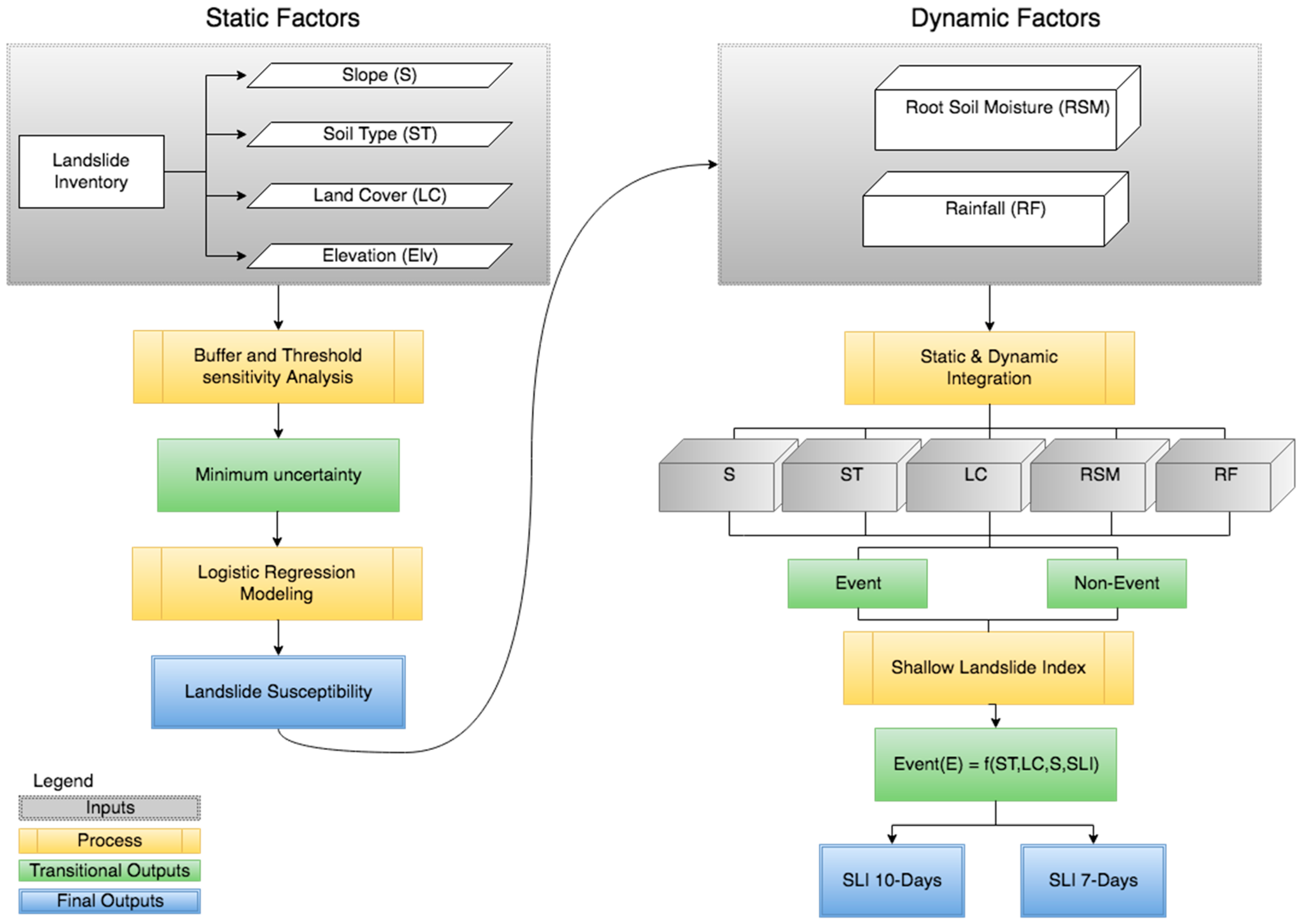
2. Materials and Methods
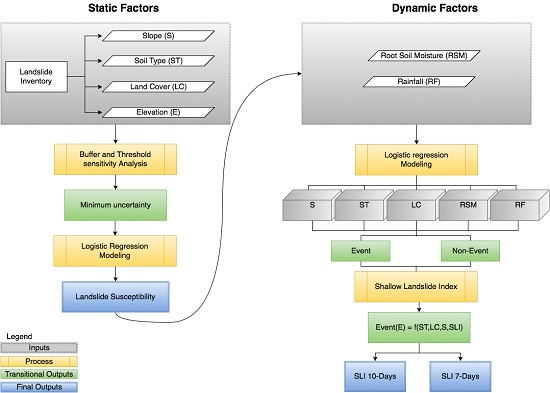
2.1. Static Factors
2.2. Dynamic Factors
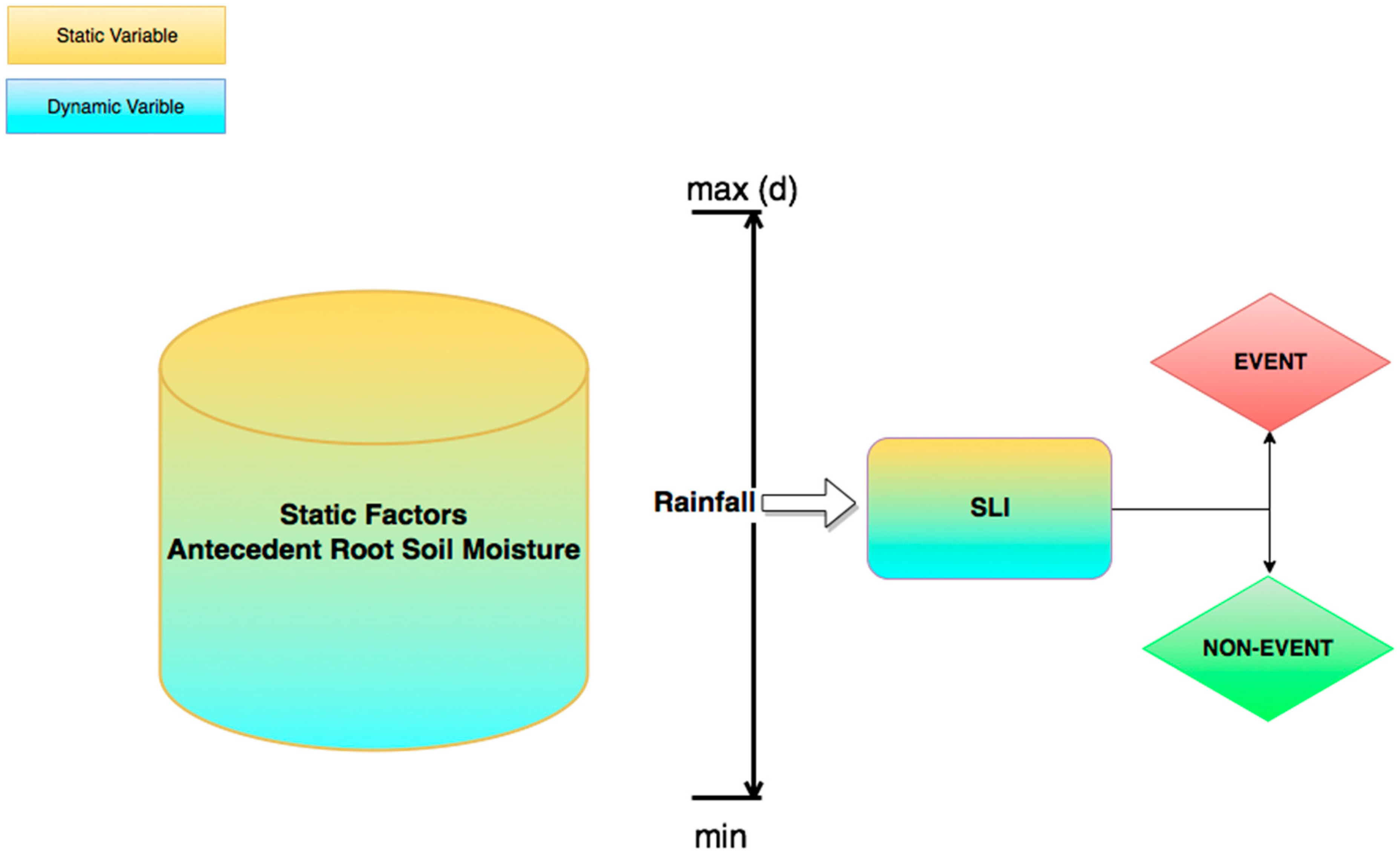
2.3. Shallow Landslide Index
2.3.1. Shallow Landslide Index Modeling
2.3.2. Assumptions and Limitations
- There are two known failure mechanisms associated with infiltration processes, in the first mechanism pore pressure increases due to liquefaction of the material, in the second mechanism, the soil remains in an unsaturated state but failure happens due to reduced suction [25]. This model assumes the first mechanism.
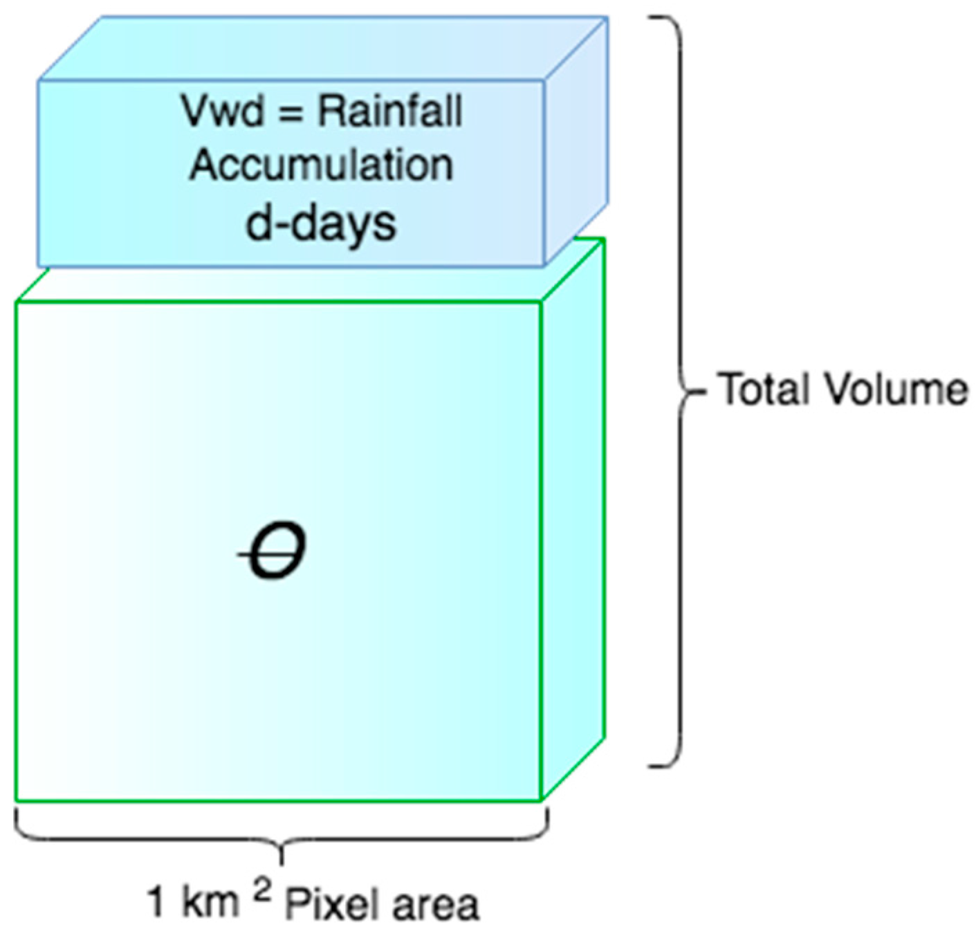
- As a data-driven model, β, the percentage of percolation is assumed to be intrinsic to all static variables in the model. It is assumed that the satellite values represent the actual moisture content in the soil after being affected by all the processes related to runoff, evaporation, suction, and percolation.
- Daily rainfall and soil moisture temporal resolutions are assumed because there is a date, not a time stamp for shallow landslide events listed in the inventory used in this study. At the moment, it is not possible to obtain a better temporal accuracy to build a large extent model based on the inventory limitations.
- Root-soil moisture (1 m) for AMSR-E and SMAP is the assumed soil moisture depth for this study.
- The L4_SM algorithm does not provide brightness temperature readings from SMAP in mountainous regions such as the Rocky Mountains or near water bodies. In areas where SMAP is not able to acquire data, root-soil moisture values are the result of forcing data and a catchment model.
2.3.3. Model Evaluation
2.3.4. Cut-off Probability
3. Results
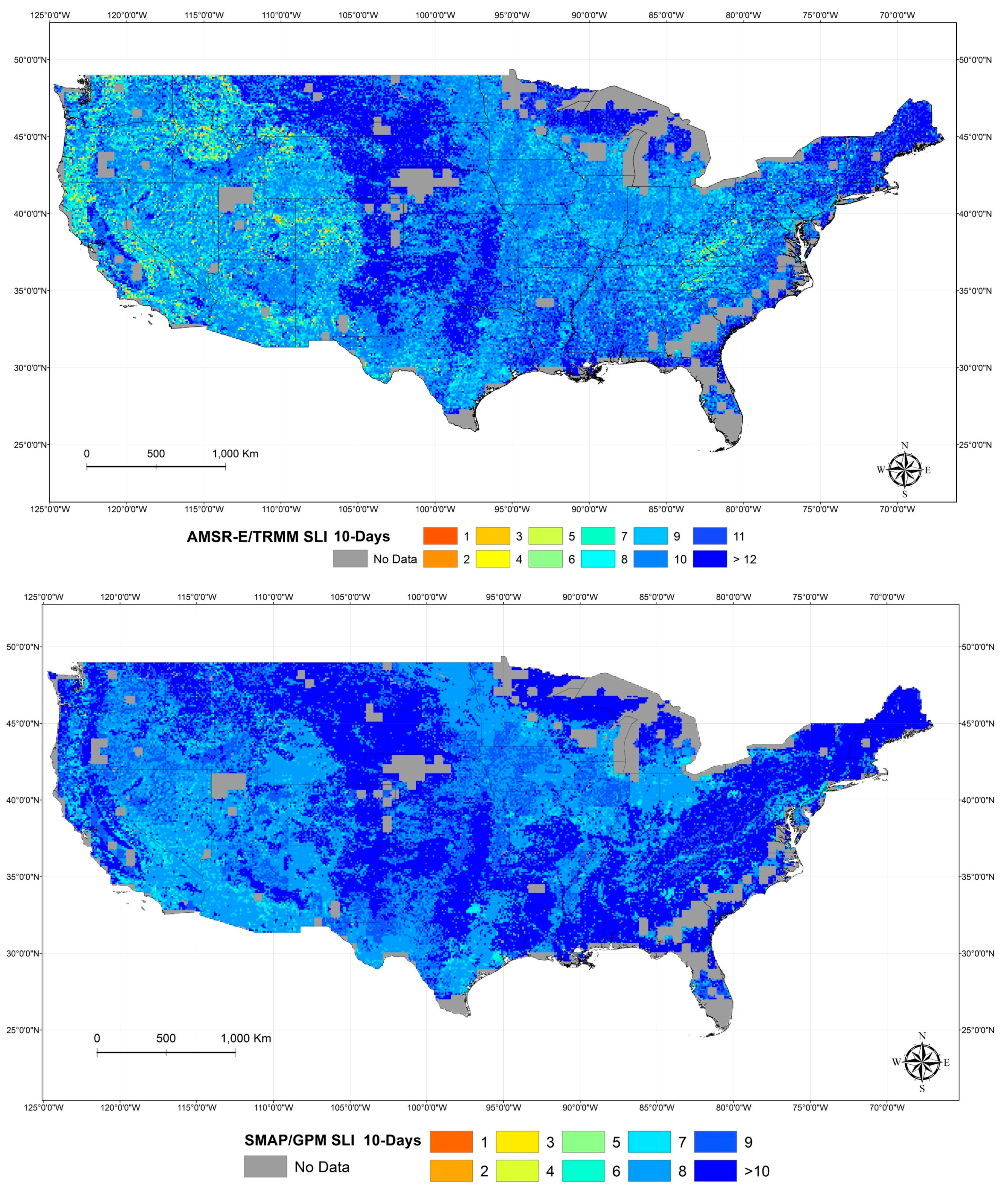
3.1. Shallow Landslide Index—AMSR-E/TRMM
3.2. Shallow Landslide Index—SMAP/GPM
3.3. SLI Application
4. Discussion
4.1. Comparing AMSR-E/TRMM and SMAP/GPM
4.2. Challenges and Limitations
5. Conclusions
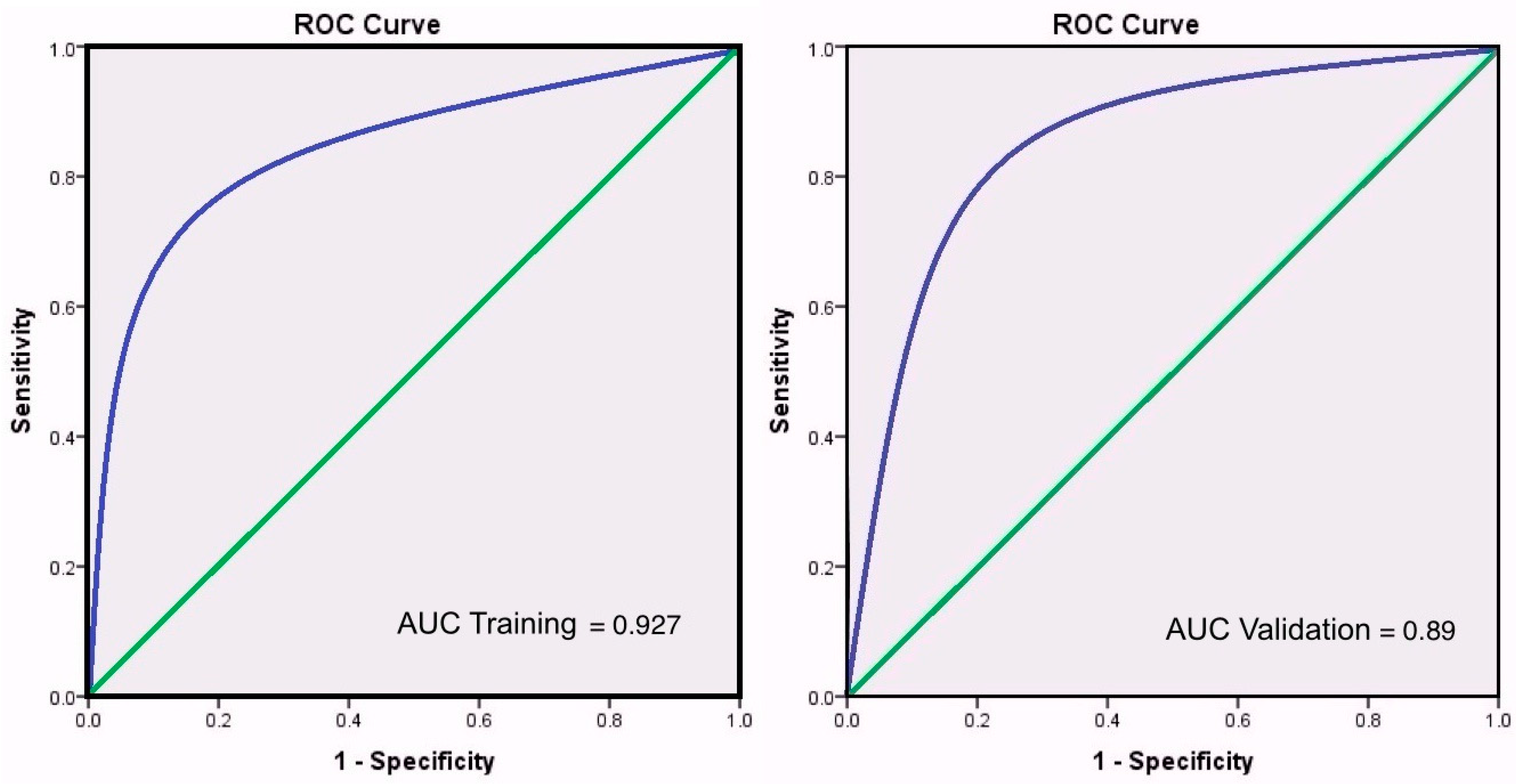
- The AMSR-E model predicts the highest number of cases correctly at 92.7% accuracy.
- The RMSE between the resulting SLI and the actual events is 0.83 in a scale from 1–13.
- The resulting index map is useful to have an understanding of hazardous areas as precedent soil moisture conditions and rainfall are taken into consideration. Nevertheless, as AMSR-E is no longer functional, current and future guidance is not possible.
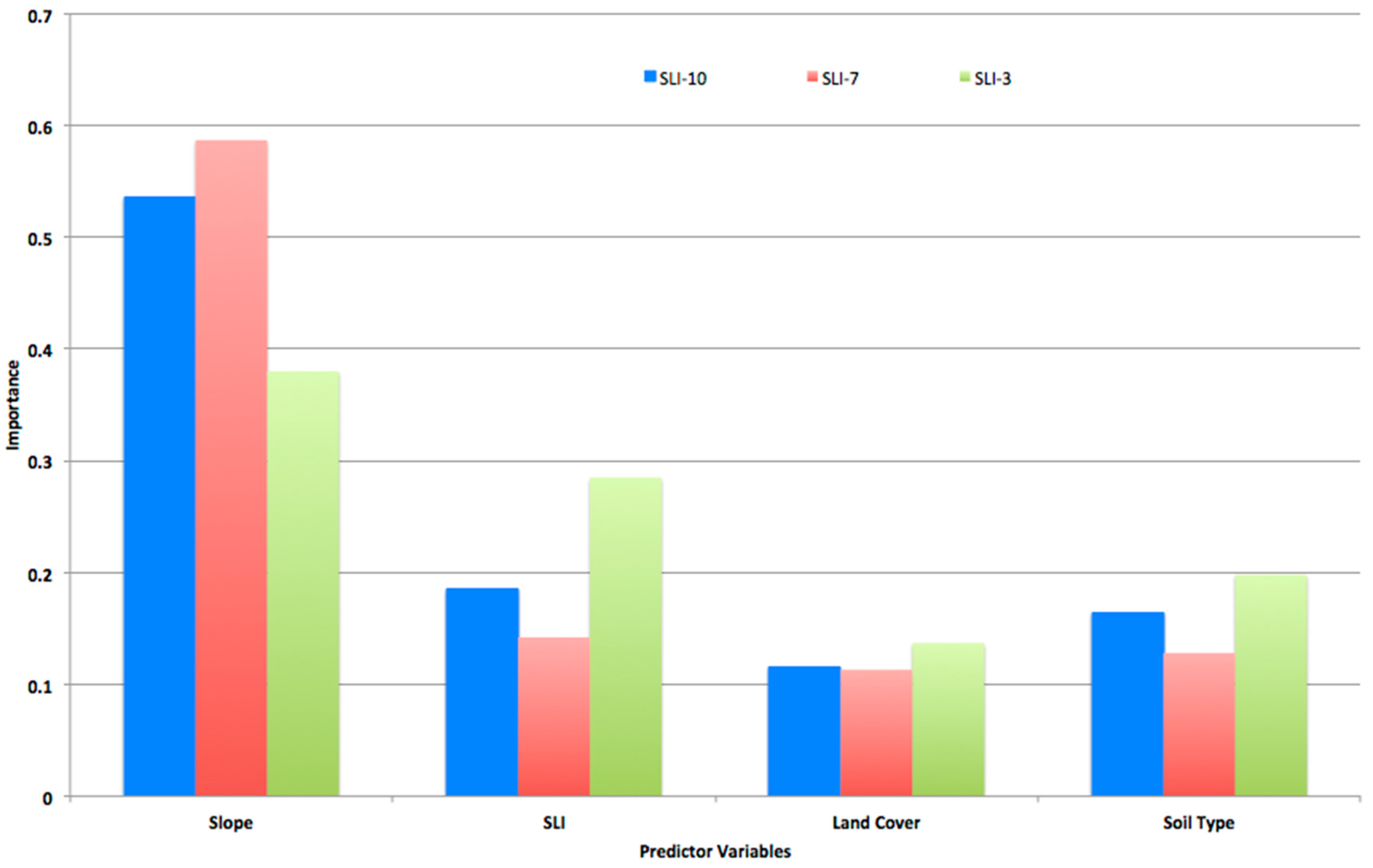
- Slope is the variable with most influence over the model followed by soil moisture content and rainfall in the form of SLI, soil type, and land cover are subsequently in importance in the three models.
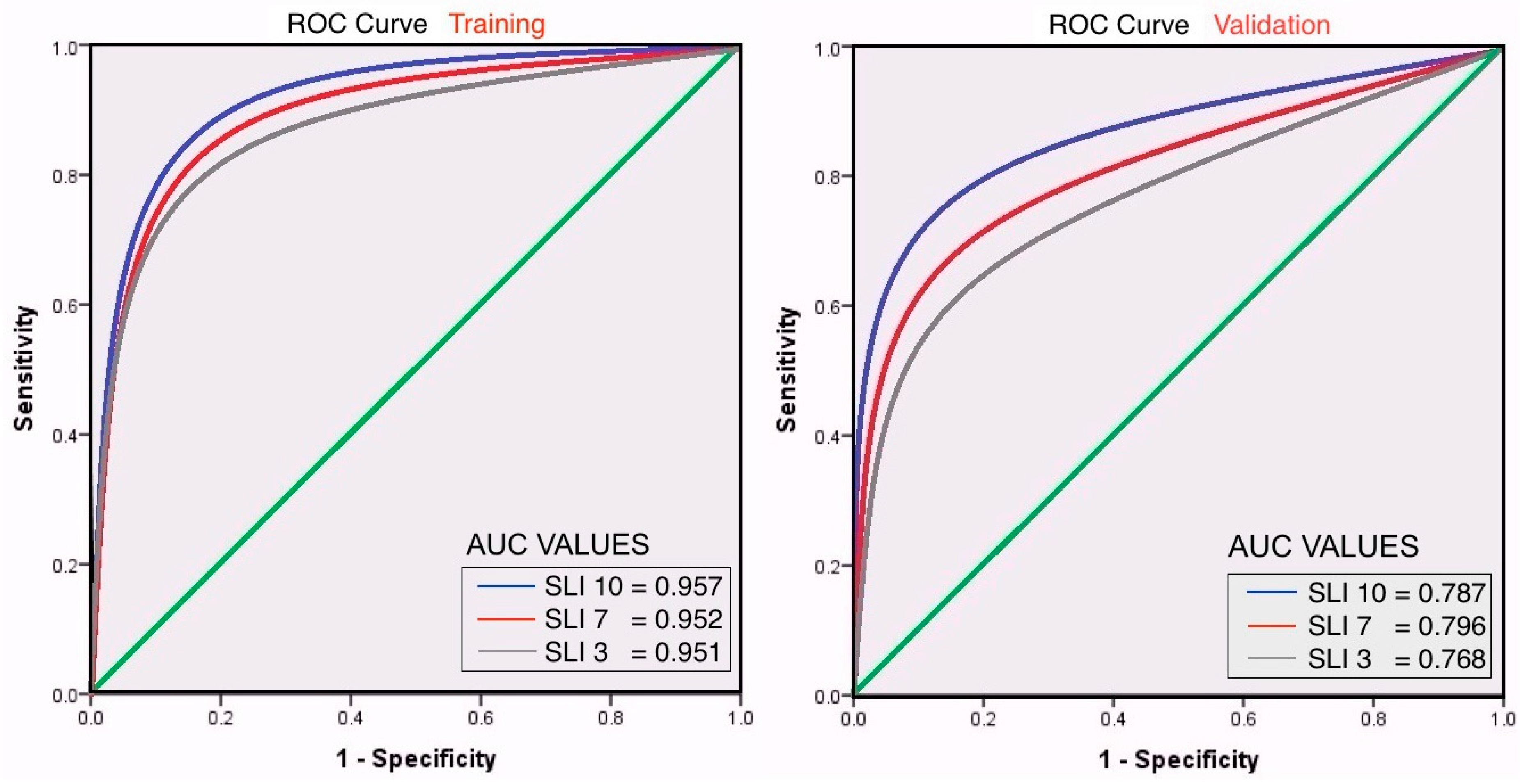
- The pseudo R2, the Nagelkerke R2 fit for a logistic regression for each model—10-day, 7-day, and 3-day—indicates a strong relationship (78.7%, 79.6%, and 76.8% respectively) between the predictors and the prediction.
- The optimal cut-off value for these logistic regression models as indicated by the AUC is 0.2.
- The RMSE is used to understand the difference between the events and the predicted SLI value for the three models, as the RMSE is scale dependent, RMSE = 1.08, 0.84, 0.97 are considered a low error in the SLI scale of 1–13.
- Comparing AMSR-E’s performance to SMAP’s is not possible even though both models are built with the same predefined static variables. There is no overlap between AMRS-E and SMAP. In addition, the sample sizes of each instrument are very different, seven years of AMSR-E and TRMM versus nine months of SMAP and GPM. Nevertheless, the t-test of significant difference in means and the f-test for significant variance result in significant differences.
Acknowledgments
Author Contributions
Conflicts of Interest
References
- Hong, Y.H.Y.; Adler, R.F.; Huffman, G. An experimental global prediction system for rainfall-triggered landslides using satellite remote sensing and geospatial datasets. IEEE Trans. Geosci. Remote Sens. 2007, 45, 1671–1680. [Google Scholar] [CrossRef]
- Kirschbaum, D.B.; Adler, R.; Hong, Y.; Hill, S.; Lerner-Lam, A. A global landslide catalog for hazard applications: Method, results, and limitations. Nat. Hazards 2009, 52, 561–575. [Google Scholar] [CrossRef]
- Cullen, C.; Kashuk, S.; Al-Suhili, R.; Khanbilvardi, R. A multistage technique to minimize overestimations of slope susceptibility at large spatial scales. J. Remote Sens. GIS 2016, 5, 159. [Google Scholar]
- Aristizábal, E.; Velez, J.; Martínez, C.; Jaboyedoff, M. SHIA_Landslide: A distributed conceptual and physically based model to forecast the temporal and spatial occurrence of shallow landslides triggered by rainfall in tropical and mountainous basins. Landslides 2016, 13, 497–517. [Google Scholar] [CrossRef]
- Oku, Y.; Nakakita, E. Future change of the potential landslide disasters as evaluated from precipitation data simulated by MRI-AGCM3.1. Hydrol. Process. 2013, 27, 3332–3340. [Google Scholar] [CrossRef]
- Barbi, F.; da Costa Ferreira, L. Risks and political responses to climate change in Brazilian coastal cities. J. Risk Res. 2013, 17, 485–503. [Google Scholar] [CrossRef]
- Chae, B.-G.; Kim, M.-I. Suggestion of a method for landslide early warning using the change in the volumetric water content gradient due to rainfall infiltration. Environ. Earth Sci. 2011, 66, 1973–1986. [Google Scholar] [CrossRef]
- Prokešová, R.; Medveďová, A.; Tábořík, P.; Snopková, Z. Towards hydrological triggering mechanisms of large deep-seated landslides. Landslides 2012, 10, 239–254. [Google Scholar] [CrossRef]
- Lehmann, P.; Gambazzi, F.; Suski, B.; Baron, L.; Askarinejad, A.; Springman, S.M.; Holliger, K.; Or, D. Evolution of soil wetting patterns preceding a hydrologically induced landslide inferred from electrical resistivity survey and point measurements of volumetric water content and pore water pressure. Water Resour. Res. 2013, 49, 7992–8004. [Google Scholar] [CrossRef]
- Crosta, G.B.; Frattini, P. Distributed modelling of shallow landslides triggered by intense rainfall. Nat. Hazards Earth Syst. Sci. 2003, 3, 81–93. [Google Scholar] [CrossRef]
- Collins, B.D.; Znidarcic, D. Stability Analyses of Rainfall Induced Landslides. J. Geotech. Geoenviron. Eng. 2004, 130, 362–372. [Google Scholar] [CrossRef]
- Segoni, S.; Rosi, A.; Rossi, G.; Catani, F.; Casagli, N. Analysing the relationship between rainfalls and landslides to define a mosaic of triggering thresholds for regional-scale warning systems. Nat. Hazards Earth Syst. Sci. 2014, 14, 2637–2648. [Google Scholar] [CrossRef]
- Segoni, S.; Rossi, G.; Rosi, A.; Catani, F. Landslides triggered by rainfall: A semi-automated procedure to define consistent intensity–duration thresholds. Comput. Geosci. 2014, 63, 123–131. [Google Scholar] [CrossRef]
- Floris, M.; Bozzano, F. Evaluation of landslide reactivation: A modified rainfall threshold model based on historical records of rainfall and landslides. Geomorphology 2008, 94, 40–57. [Google Scholar] [CrossRef]
- Brunetti, M.T.; Peruccacci, S.; Rossi, M.; Luciani, S.; Valigi, D.; Guzzetti, F. Rainfall thresholds for the possible occurrence of landslides in Italy. Nat. Hazards Earth Syst. Sci. 2010, 10, 447–458. [Google Scholar] [CrossRef]
- Giannecchini, R.; Galanti, Y.; D’Amato Avanzi, G. Critical rainfall thresholds for triggering shallow landslides in the Serchio River Valley (Tuscany, Italy). Nat. Hazards Earth Syst. Sci. 2012, 12, 829–842. [Google Scholar] [CrossRef]
- Papa, M.N.; Medina, V.; Ciervo, F.; Bateman, A. Derivation of critical rainfall thresholds for shallow landslides as a tool for debris flow early warning systems. Hydrol. Earth Syst. Sci. 2013, 17, 4095–4107. [Google Scholar] [CrossRef]
- Kirschbaum, D.; Stanley, T.; Yatheendradas, S. Modeling landslide susceptibility over large regions with fuzzy overlay. Landslides 2016, 13, 485–496. [Google Scholar] [CrossRef]
- Baum, R.L.; Godt, J.W. Early warning of rainfall-induced shallow landslides and debris flows in the USA. Landslides 2009, 7, 259–272. [Google Scholar] [CrossRef]
- Kirschbaum, D.; Adler, R.; Hong, Y. Advances in landslide nowcasting: Evaluation of a global and regional modeling approach. Environ. Earth Sci. 2012, 66, 1683–1696. [Google Scholar] [CrossRef]
- Glade, T.; Crozier, M.; Smith, P. Applying probability determination to refine landslide-triggering rainfall thresholds using an empirical “Antecedent Daily Rainfall Model”. Pure Appl. Geophys. 2000, 157, 1059–1079. [Google Scholar] [CrossRef]
- Liao, Z.; Hong, Y.; Wang, J.; Fukuoka, H.; Sassa, K.; Karnawati, D.; Fathani, F. Prototyping an experimental early warning system for rainfall-induced landslides in Indonesia using satellite remote sensing and geospatial datasets. Landslides 2010, 7, 317–324. [Google Scholar] [CrossRef]
- Brocca, L.; Ponziani, F.; Moramarco, T.; Melone, F.; Berni, N.; Wagner, W. Improving Landslide Forecasting Using ASCAT-Derived Soil Moisture Data: A Case Study of the Torgiovannetto Landslide in Central Italy. Remote Sens. 2012, 4, 1232–1244. [Google Scholar] [CrossRef]
- Chen, H.X.; Zhang, L.M. A physically-based distributed cell model for predicting regional rainfall-induced shallow slope failures. Eng. Geol. 2014, 176, 79–92. [Google Scholar] [CrossRef]
- Aristizábal, E.; García, E.; Martínez, C. Susceptibility assessment of shallow landslides triggered by rainfall in tropical basins and mountainous terrains. Nat. Hazards 2015, 78, 621–634. [Google Scholar] [CrossRef]
- Godt, J.W.; Baum, R.L.; Chleborad, A.F. Rainfall characteristics for shallow landsliding in Seattle, Washington, USA. Earth Surf. Process. Landf. 2006, 31, 97–110. [Google Scholar] [CrossRef]
- Van Westen, C.J.; Castellanos, E.; Kuriakose, S.L. Spatial data for landslide susceptibility, hazard, and vulnerability assessment: An overview. Eng. Geol. 2008, 102, 112–131. [Google Scholar] [CrossRef]
- Land, G.; Share, C.; Latham, J.; Cumani, R.; Rosati, I.; Bloise, M. Global Land Cover SHARE. Available online: http://www.glcn.org/downs/prj/glcshare/GLC_SHARE_beta_v1.0_2014.pdf (accessed on 18 October 2016).
- Goddard Earth Sciences Data and Information Services Center (GES DISC). TRMM (TMPA) Precipitation L3 1 day 0.25 Degree × 0.25 Degree V7. 2010. Available online: http://disc.sci.gsfc.nasa.gov/datacollection/TRMM_3B42_daily_V7.html (accessed on 18 October 2016). [Google Scholar]
- GES DISC. TRMM TMPA. 2015. Available online: http://mirador.gsfc.nasa.gov/cgi-bin/mirador/presentNavigation.pl?tree=project (accessed on 18 October 2016). [Google Scholar]
- Ray, R.L.; Jacobs, J.M.; Ballestero, T.P. Regional landslide susceptibility: Spatiotemporal variations under dynamic soil moisture conditions. Nat. Hazards 2011, 59, 1317–1337. [Google Scholar] [CrossRef]
- Guns, M.; Vanacker, V. Logistic regression applied to natural hazards: Rare event logistic regression with replications. Nat. Hazards Earth Syst. Sci. 2012, 12, 1937–1947. [Google Scholar] [CrossRef]
- Food and Agriculture Organization of the United Nations (FAO); Applied International Institute for Systems Analysis (IIASA); ISRIC-World Soil Information; Institute of Soil Science—Chinese Academy of Sciences (ISSCAS); Joint Research Centre of the European Commission (JRC). Harmonized World Soil Database; FAO: Rome, Italy; IIASA: Laxenburg, Austria, 2012. [Google Scholar]
- Entekhabi, D.; Yueh, S.; O’Neill, P.E.; Kellogg, K.H. SMAP Handbook JPL 400-1567. 2014. Available online: https//smap.jpl.nasa.gov/files/smap2/SMAP_Handbook_FINAL_1_JULY_2014_Web.pdf (accessed on 18 October 2016). [Google Scholar]
- International Business Machines Corporation (IBM). SPSS; IBM: Armonk, NY, USA, 2013. [Google Scholar]
- Longoni, L.; Papini, M.; Brambilla, D.; Arosio, D.; Zanzi, L. The role of the spatial scale and data accuracy on deep-seated gravitational slope deformation modeling: The Ronco landslide, Italy. Geomorphology 2016, 253, 74–82. [Google Scholar] [CrossRef]
- Kimball, J.S.; Jones, L.A.; Glassy, J.; Stavros, E.N.; Madani, N.; Reichle, R.H.; Jackson, N.T.; Colliander, A. Soil Moisture Active Passive Mission L4_C Data Product Assessment (Version 2 Validated Release). 2016. Available online: https://gmao.gsfc.nasa.gov/pubs/docs/Kimball852.pdf (accessed on 18 October 2016). [Google Scholar]


| Soil Type | Shape Area km2 | Number of Events | Random Points |
|---|---|---|---|
| Cambisols | 718,950 | 65 | 400 |
| Luvisols | 2,953,072 | 60 | 591 |
| Acrisols | 1,746,111 | 44 | 110 |
| Phaeozems | 1,188,000 | 17 | 202 |
| Kastanozems | 2,427,042 | 13 | 316 |
| Andosols | 318,317 | 12 | 50 |
| Podzols | 699,157 | 10 | 44 |
| Regosols | 761,849 | 9 | 40 |
| Total Cases | 1753 | ||||
|---|---|---|---|---|---|
| Event | Number of Cases | Total % of Data | % Cases Modeled | % Event Model Cases | Number of Cases |
| 1 | 141 | 8 | 141/1263 = 11 | 141/204 = 69 | 1263 |
| 0 | 1122 | 64 | 1122/1263 = 89 | 1122/1549 = 72 | |
| 1263 | 72 | 72% | |||
| Event | Number of Cases | % Total | % Cases Validated | % Event Validated Cases | Number of Cases |
| 1 | 63 | 3.6 | 63/490 = 12.8 | 63/204 = 31 | 490 |
| 0 | 427 | 24.3 | 427/490 = 87.2 | 427/1549 = 27.6 | |
| 490 | 27.9 | 28% | |||
| Shallow Landslide Event | ||||
|---|---|---|---|---|
| Predicted | Not Predicted | Total | ||
| Landslide | 116 true positive | 8 false positive | 128 | |
| Not landslide | 12 false negative | 1103 true negative | 1111 | |
| Total | 128 | 1111 | 1239 | |
| Model | Chi-Square | Df. | Sig. |
|---|---|---|---|
| 10-day | 155.484 | 4 | 0.000 |
| 7-day | 156.208 | 4 | 0.000 |
| 3-day | 156.552 | 4 | 0.000 |
| Descriptive Statistics | |||||||||
|---|---|---|---|---|---|---|---|---|---|
| N | Min. | Max. | Mean | Std. | Var. | Skewness | |||
| ST | ST | ST | ST | Std. Error | ST | ST | ST | Std. Error | |
| SLI_10_Day | 3837 | 6 | 13 | 9.48 | 0.025 | 1.54 | 2.373 | 0.222 | 0.04 |
| AMSR-E | 3837 | 1 | 13 | 9.08 | 0.026 | 1.63 | 2.656 | −0.803 | 0.04 |
| Mean | Std. Dev. | Std. Error Mean | t. | Df. | Sig. (2-Tailed) | |
|---|---|---|---|---|---|---|
| Models | 0.39927 | 1.356 | 0.0218 | 18.238 | 3836 | 0.000 |
© 2016 by the authors; licensee MDPI, Basel, Switzerland. This article is an open access article distributed under the terms and conditions of the Creative Commons Attribution (CC-BY) license (http://creativecommons.org/licenses/by/4.0/).
Share and Cite
Avalon Cullen, C.; Al-Suhili, R.; Khanbilvardi, R. Guidance Index for Shallow Landslide Hazard Analysis. Remote Sens. 2016, 8, 866. https://doi.org/10.3390/rs8100866
Avalon Cullen C, Al-Suhili R, Khanbilvardi R. Guidance Index for Shallow Landslide Hazard Analysis. Remote Sensing. 2016; 8(10):866. https://doi.org/10.3390/rs8100866
Chicago/Turabian StyleAvalon Cullen, Cheila, Rafea Al-Suhili, and Reza Khanbilvardi. 2016. "Guidance Index for Shallow Landslide Hazard Analysis" Remote Sensing 8, no. 10: 866. https://doi.org/10.3390/rs8100866
APA StyleAvalon Cullen, C., Al-Suhili, R., & Khanbilvardi, R. (2016). Guidance Index for Shallow Landslide Hazard Analysis. Remote Sensing, 8(10), 866. https://doi.org/10.3390/rs8100866