Remote Sensing from Ground to Space Platforms Associated with Terrain Attributes as a Hybrid Strategy on the Development of a Pedological Map

Abstract

There is a consensus about the necessity to achieve a quick soil spatial information with few human resources. Remote/proximal sensing and pedotransference are methods that can be integrated into this approach. On the other hand, there is still a lack of strategies indicating on how to put this in practice, especially in the tropics. Thus, the objective of this work was to suggest a strategy for the spatial prediction of soil classes by using soil spectroscopy from ground laboratory spectra to space images platform, as associated with terrain attributes and spectral libraries. The study area is located in São Paulo State, Brazil, which was covered by a regular grid (one per ha), with 473 boreholes collected at top and undersurface. All soil samples were analyzed in laboratory (granulometry and chemical), and scanned with a VIS-NIR-SWIR (400–2500 nm) spectroradiometer. We developed two traditional pedological maps with different detail levels for comparison: TFS-1 regarding orders and subgroups; and TFS-2 with additional information such as color, iron and fertility. Afterwards, we performed a digital soil map, generated by models, which used the following information: (i) predicted soil attributes from undersurface layer (diagnostic horizon), obtained by using a local spectral library; (ii) spectral reflectance of a bare soil surface obtained by Landsat image; and (iii) derivative of terrain attributes. Thus, the digital map was generated by a combination of three variables: remote sensing (Landsat data), proximal sensing (laboratory spectroscopy) and relief. Landsat image with bare soil was used as a first observation of surface. This strategy assisted on the location of topossequences to achieve soil variation in the area. Afterwards, spectral undersurface information from these locations was used to modelize soil attributes quantification (156 samples). The model was used to quantify samples in the entire area by spectra (other 317 samples). Since the surface was bare soil, it was sampled by image spectroscopy. Indeed, topsoil spectral laboratory information presented great similarity with satellite spectra. We observed angle variation on spectra from clayey to sandy soils as differentiated by intensity. Soil lines between bands 3/4 and 5/7 were helpful on the link between laboratory and satellite data. The spectral models of soil attributes (i.e., clay, sand, and iron) presented a high predictive performance (R² 0.71 to 0.90) with low error. The spatial prediction of these attributes also presented a high performance (validations with R² > 0.78). The models increased spatial resolution of soil weathering information using a known spectral library. Elevation (altitude) improved mapping due to correlation with soil attributes (i.e., clay, iron and chemistry). We observed a close relationship between soil weathering index map and laboratory spectra + image spectra + relief parameters. The color composite of the 5R, 4G and 3B had great performance on the detection of soils along topossequences, since colors went from dark blue to light purple, and were related with soil texture and mineralogy of the region. The comparison between the traditional and digital soil maps showed a global accuracy of 69% for the TFS-1 map and 62% in the TFS-2, with kappa indices of 0.52 and 0.45, respectively. We randomly validated both digital and traditional maps with individual plots at field. We achieve a 75% and 80% agreement for digital and traditional maps, respectively, which allows us to conclude that traditional map is not necessarily the truth and digital is very close. The key of the strategy was to use bare soil image as a first step on the indication of soil variation in the area, indicating in-situ location for sample collection in all depths. The current strategy is innovative since we linked sensors from ground to space in addition with relief parameters and spectral libraries. The strategy indicates a more accurate map with less soil samples and lower cost.

1. Introduction

The basis for every agricultural system is the land use planning. Brazil has about 270,000 million ha of agriculture lands and only 17% of this has been properly used. Mendonça-Santos [1] and Santos [2] indicate that Brazil has only between 0.25% and 1% of soils mapped in a semi-detailed or detailed scale (1:20,000), which is most important for agriculture. With exception of the United States, most of the world has very few maps that are suitable for agriculture. The pedological map is related to the spacialization of soil class units and reveals the variation of several characteristics, such as texture, fertility, organic matter, depth, pedregosity and water dynamics. These are the most important types of information for crop growing, environment monitoring and land use planning.

During the last decades, a concentration on soils basic concepts study (i.e., genesis, and weathering) led to the proper development of soil taxonomy and classification. This approach has been the basis of soil mapping, but took community to focus on punctual soil information (the profile), and let less research on its spatial distribution (maps). Indeed, a recent review [3] shows the importance of pedological mapping as a recent issue. In conventional soil mapping, several issues are habitual such as hard fieldwork, great time demand and high costs on soil analysis. These issues took community to observe the importance on taking into account new technologies such as remote and proximal sensing, Digital Soil Mapping (DSM) and Digital Soil Morphometrics [4,5,6,7].

On the other hand, as indicated by [8], soil sensing has become the new paradigm in agriculture. Indeed, soil sensing could facilitate the measurement and monitoring of soil attributes for better understand its dynamics, but we still have to breakdown old concepts on soil mapping. Santos et al. [2] stated that, in 1990, Brazil had few soil mapping works due to economic, technical and methodological reasons.

The usual methodology carries basic principles of soil mapping [8]. On the other hand, several subjectivities come from pedologists, and conventional soil maps are not exempt of error. Filho et al. [9] demonstrated that five pedologists developed different soil maps in the same area, indicating the necessity to insert some technology to diminish this variation. In many cases, the soil mappers faces complex problems and must make empirical decisions based on their knowledge to decide soil limits or classification. Some investigations indicated that in conventional soil mapping, the purity of soil units is frequently low [10,11]. Dobos et al. [12] estimated a taxonomic purity of 49.1% for the soil and terrain information in Hungary. The database was created using the traditional, expert-knowledge-based method [13].

In this way, DSM arose to overcome the problems associated with traditional mapping, and its essence was firstly introduced by [14], as well as properly discussed in [15,16,17]. Commonly, DSM has focused on the survey of large areas [18], since time, cost and human resources represent enormous challenges. DSM systems can insert several variables to reach the main goal, such as remote sensing information, relief parameters, geology and others.

Several strategies have been used for developing the DSM. Regardless of soil spectroscopy, first findings on pedological mapping were performed by [19]. They based their vision on the spectroscopy principles to characterize soil classes and afterwards specialization by relief. Indeed, spectroscopy quantifies important soil attributes looking for soil classification [20,21]. This strategy also indicates its usefulness for soil classification as performed by a multi-depth spectral analysis [22]. The use of spectral libraries are an important strategy for attributes quantification, as performed by Shepherd, K.D.; Walsh [21] and Shi et al. [23]. Additionally, spectral libraries have also been used on soil classification [22,24,25].

Observing soils from top, the use of aerial hyperspectral images has also been addressed by [26], as well as by multispectral satellite sensing [27]. Relief parameters were also used for pedological mapping as indicated by [28]. In fact, prior to the use of hyperspectral imaging, there have been a number of studies using multispectral images either by visual interpretation or by digital processing throughout 1970–2000s [13,29,30,31].

Thus, many sources can assist soil mapping. Soil spectroscopy have a great potential to assist DSM because can provide accurate soil information, being faster and cheaper than the conventional methods for soil analysis. Nocita et al. [32] indicate the importance of these technologies to optimize soil analysis. Vasques et al. [22,33] determined important methods on soil class discrimination by spectra. Later Vasques et al. [34] suggested a strategy for pedological mapping using relief, spectra and stream density reaching 85% accuracy.

Recent results (e.g., [35]) achieved 76.3% of agreement using spectroscopy for soil classification. However, there is still a lack of strategies on how to use these tools simultaneously to generate soil maps in large scale. In contrast, detailed soil maps could considerably increase productivity in intensive crops. Towards these findings, Lepsch describes the necessity of large-scale soil information for agriculture in Brazil [36].

Most papers indicate great importance of each technique, but isolated from themselves (spectroscopy, images or relief). On the other hand, during the delineation of a soil map, there are various strategies depending on the products available for users, which depend on the complexity of a given area and the experience of the pedologist. Indeed, pedologists merge all the information (punctual, spatial, relief, color, etc.) to make a map. Therefore, it is worth to use a similar strategy with tools we have currently available.

In our view, there are few works with a focus on detailed pedologic mapping using several techniques to reach the goal. In addition, despite the development of spectral libraries, it is important to show how to use them for this purpose [24]. Therefore, we must merge the punctual information as described by Digital Soil Morphometrics [7] discipline with the spatial domain on DSM.

Based on these observations, the objective of this work was to determine a detailed pedological map using a strategy sustained on the combination of soil spectroscopy by ground and satellite information, and terrain parameters, all used for pedotransference concept. The acquisition and determination of large-scale soil map is dependent on pedological concepts. Considering this information, the present work used a great amount of point-by-point topographical information, which allowed soil discrimination and classification by digital tools. We expect to achieve a digital soil technique that uses rapid soil analysis with high quality of delineation. The work could bring light to the importance of large-scale maps determined by multi task strategy.

2. Materials and Methods

2.1. Study Site, Sampling and Soil Characterization

The study area is located at the Barra Bonita city, southeast of São Paulo State (Figure 1). The site comprises an area of 473 ha cultivated with sugar cane for the last 30 years. The climate corresponds to subtropical mesotermic according to Köppen classification [37]. The predominant parental materials are sandstone intercalated with intrusive bodies of tholeitic basalts from Serra Geral Formation [38].

The area was covered by a regular sampling grid with 100 × 100 m² spacing (one sample per ha). Soils were sampled at two depths (0–0.2 and 0.8–1.0 m) by auger, considered in this study as top surface and undersurface diagnostic horizons, respective, performing a total of 946 samples. Soil chemical analysis were performed according to [39], and particle size distribution and sulfuric acid digestion according to [40,41]. The following attributes were determined: Ca, Mg, K, sum of bases (BS), clay, silt, sand, total Al (Al₂O₃), total free-Fe (Fe₂O₃), Al₂O₃/Fe₂O₃ ratio, silica (expressed as SiO₂), titanium (expressed as TiO₂), index of the weathering stage and weathering index. The weathering indexes used were silt/clay and ki (1.7 SiO₂/Al₂O₃). The Ki index represents the soil weathering degree, where Ki > 3 indicate less weathered soils (2:1 mineral soils: vermiculite and montmorillonite); 2 < Ki < 3 indicate intermediate weathered soils (kaolinitic dominance); Ki ≤ 2 indicate more weathered soils (kaolinitic and oxidic); and Ki ≤ 0.75 indicate highly weathered soils (gibsitic and kaolinitic) [42].

The conventional soil map was based on a traditional field survey (TFS) and was developed in two different detailing levels [2,8]. The Brazilian Soil Classification [42] was used and then transformed into Soil Taxonomy Classification for this paper [43]. These maps were developed by 473 boreholes samplings and 20 pits (sample collected in horizon’s soil profile), all characterized by laboratorial analysis. The first TFS map (TFS-1) contains information regarding soil order to subgroups. The second map (TFS-2) contains additional information related to soil attributes such as color, iron and fertility levels. TFS-1 and TFS-2 are considered as detailed level maps (1:20,000 scale) by traditional systems, with high-density sampling, i.e., 1 observation ha⁻¹.

2.2. Soil Database for Digital Mapping

The information used for digital soil mapping corresponds to three datasets: satellite image (remote sensing spectra, DsSB), terrain attributes from a digital elevation model (DsTP) and proximal sensing spectra (laboratorial spectra, DsSA). Each of these information sources contributes to describe a different aspect from soils at site. DsSB were important to describe spatial variation at soil surface. Terrain attributes from DsTP were important information for spatial prediction of soil classes. The DsSA spectra were used for undersurface horizon, since the image only brings surface information.

The DsSB corresponded to a Landsat-5 TM image, which was previously geo-referenced, geometrically and atmospherically corrected and the signal was converted to reflectance [44]. The image date correspond to 27 August 1997, when all the site had bare soil as well as low moisture, due to the season of sampling. The area was completely plowed without vegetation or straw at ground. Field samples were collected at the same period of the image.

The DsTP was developed based on a digital elevation model (DEM) with 5 m resolution, which was obtained by contour interpolation of the segment map using a linear algorithm. In order to improve the plausibility of the DEM, it was pre-processed according to [45]. To reduce the outliers the DEM was filtered by using a 3 × 3 window, which used the kriging weights calculated from the semi-variogram of elevation. The kriged elevation values were compared with the original values and a map of normalized residuals was obtained and used to produce the final smoothed DEM. Two terrain attributes was derived from the DEM: slope and mean curvature. These parameters were chosen because they are related to soil thickness, depositional gains, erosional losses, oxidation-reduction process, which are related with soil formation.

To establish the DsSA dataset, the soil samples were dried at 45 °C for 24 h and sieved (2 mm mash). Soils spectra were obtained in laboratory with Infra-Red Intelligent Spectroradiometer (IRIS) sensor (Geophysical and Environmental Research Corporation) with resolutions of 2 nm in the range from 350 to 1000 nm (VIS-NIR) and 4 nm from 1000 to 2500 nm (SWIR). The sensor was positioned vertically at a distance of 27 cm over the soil sample. The samples were placed in a 9 cm petri dish, forming a 1.5 cm layer of soil. The light source corresponded to a 600 W halogen lamp positioned 61 cm from the sample container at a 15° zenital angle. A gray plate with 50% reflectance was used for sensor calibration [46].

2.3. Undersurface Soil Attributes Quantification and Mapping

An important step on the methodology was the prediction of the undersurface soil attributes maps. In order to develop this library some chemometrical procedures were carried out. A principal component analysis (PCA) of the spectra data was performed. Outlier samples were identified using the scores of the principal components (PCs). Samples with Mahalanobis distances upper 3 were excluded from the dataset. Once the outliers were removed, a total of 206 samples were selected from transect sections. This dataset selection was performed by the conditioned Latin Hypercube Sampling method (cLHS) over the two first PC scores [47]. Later, the selected dataset was separated into 156 samples (calibration set) and 50 samples (validation set). Spatial distribution of calibration, validation and prediction sample location are presented in the Figure 1. A flowchart of the methodology is presented in Figure 2.

Models of Fe₂O₃, Al₂O₃, SiO₂, TiO₂, Clay and sum of bases (BS) were calibrated by partial least squares regression (PLSR) using the software ParLeS [48]. PLSR have been widely used showing good performance [49,50]. Pre-processing procedures were applied for laboratory spectra and then transformed to absorbance. The number of PLS factors and the pre-processing techniques employed were defined based on a cross-validation of all possible calibration models. The following fitting parameters were used to select the best models: coefficient of determination (R²), root mean square error (RMSE), mean error (ME) and standard deviation error (SDE). After the models calibration, the predictive performance was assessed based on the test set. The validation was carried out and the R², RMSE, ME and SDE were calculated again.

Once the models were validated, we used them to predict soil attributes in all sampling grid. We did this for all undersurface samples (which was expected to be the diagnostic horizon). Hence, these predictions lead to increase the spatial resolution of the soil attribute data, using only some soil transects towards a high density grid of 100 m² (Figure 1). Thus, from 156 samples used in the model (spectral versus wet analysis), we measured the other 317 only by spectra.

In the last step, we performed the spatial prediction of soil attributes, which reflects important information of soil weathering. Spatial structures of data were analyzed by geostatistical methods using the GeoR package of R software (version 2.7.2) [51]. Afterwards, we predicted the experimental semi-variograms and evaluated the spatial structure characteristics. Semi-variograms and ordinary kriging interpolation method were the basis to generate raster maps of soil attributes. Performance of spatial predictions (kriging) were evaluated by leave-one-out cross validation method. Maps of Ki index were calculated from the raster maps of SiO₂ and Al₂O₃.

2.4. Digital Mapping Strategy

We used simultaneously the information extracted from the three datasets (DsSA, DsSB and DsTP) to predict soil classes. In order to summarize the main soil information that contained the datasets (DsSA, DsSB and DsTP), a PCA of each one was carried out. Hence, the size of each dataset was reduced to a new group of variables that accounted for more than 95% of the variation between the original variables. In this way, soil raster maps (Fe₂O₃, Al₂O₃, SiO₂, TiO₂, Clay, BS and Ki) of the DsSA were reduced to a lower number of variables. DsSB data, i.e., bands 1 (450–520 nm), 2 (520–600 nm), 3 (630–690 nm), 4 (760–900 nm), 5 (1550–1750 nm) and 7 (2080–2350 nm) of the satellite image were also reduced. This same procedure was followed for the DsTP. The summarized datasets were called DsSA-PC, DsSB-PC and DsTP-PC. These data reductions were important to avoid redundancy and collinearity of the information, which could decrease the predictive performance of soil classes.

In this stage by using the field traditional soil class maps (TFS) and DsSA-PC, DsSB-PC and DsTP-PC variables, we collected the training information for the learning algorithm in order to generate a classifier. The collection of training information was carried out in two steps as follows: (i) we identified five toposequences with clearly defined soil classes along relief; and (ii) these toposequences were located in the maps of the three datasets and in the TFS maps, and the information of pixels from these toposequences were collected afterwards in image. A total of 260 pixels or training data were collected for image evaluation.

Using the pixels data collected from the five toposequences, the maximum likelihood algorithm was used to create the classification rules. This supervised classification method has shown good performance in several works [17,52]. Two classification rules were created: the first one was used to predict the TFS-1 map and the second to predict the TFS-2 map. The two classification rules were applied to the whole area and based on the DsSA-PC, DsSB-PC and DsTP-PC rasters. The first digital soil map (DSC-1) generated was equivalent to TFS-1 map, and the second one (DSC-2) was equivalente to TFS-2 map.

2.5. Comparison between Traditional (TFS) and Digital (DSC) Soil Maps

Three comparison methods were performed. The first one is called degree of spatial correspondence (DSc), which is an agreement indicator between two correspondent polygons of maps and takes into account its size. The second one is the spatial correspondence (Sc), which indicates what percentage of each traditional soil class area is covered by each digital class area. Additionally, it was evaluated the overall accuracy and the kappa index. The degree of agreement was based on the comparison of predicted and actual class labels for each case in the testing set [53]. The Kappa index is a robust index that takes into account the probability that a pixel is classified by chance. It was calculated from a confusion matrix and its values were classified as proposed by [54]. It was divided into five levels according to the performance: 0–0.2, 0.2–0.4, 0.4–0.6, 0.6–0.8, and 0.8–1.0, being, respectively, low, moderate, good, very good and excellent performance. For calculations, the predicted digital soil class maps were smoothed by using a majority filter in order to eliminate undefined pixels and areas of soil classes with low number of pixels. Figure 1, Figure 2 and Figure 3 illustrates the sequence of the method.

3. Results and Discussion

3.1. Soils in the Study Area

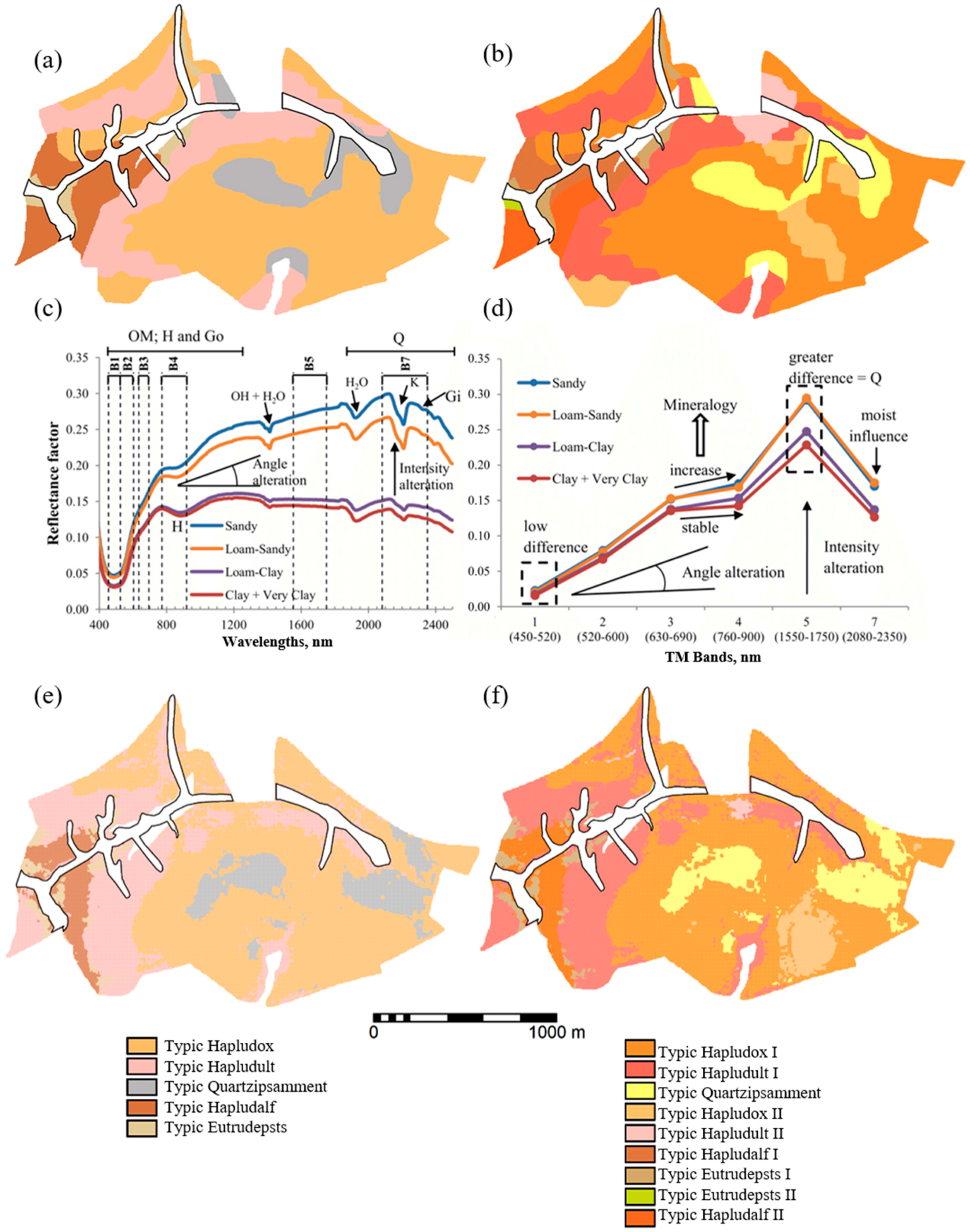
Traditional soil map with lower detail showed a heterogeneous variation of soil classes (Figure 4a). The predominant soils of the studied area were classified as: Typic Hapludox (THud), Typic Hapludalf (THa), Typic Hapludult (THu), Typic Eutrudept (TE) and Typic Quartzipsamment (TQ) [43] (

Table 1. Mean of chemical and granulometric attributes of the mapping units in the study area.

N 1	Layer 2	OM 3	K	Ca	Mg	Al	H	BS	T	V	m	Sand	Silt	Clay	Wet Color 4			Fe2O3	Ki 5
		g·kg−1	mmolc·kg−1							%		%			Hue	Value	Chroma	g·kg−1
Typic Hapludox 1 (THud1)
252	A	14.8	2.4	14.6	5.8	1.6	24.7	22.9	47.6	49.4	7.8	70.8	5.7	23.5	2.5	3.5	1.9	57.7	1.9
	B	12.3	0.8	6.1	2.3	8.2	25.4	9.3	34.6	26	45.7	64.3	4.8	30.9	1.8	3.6	2.4	66.3	1.8
Typic Hapludox 2 (THud2)
34	A	16.8	2.9	23.6	7.8	1.2	20.8	34.2	55.1	61.9	4.3	66	8	26	3	3.6	2.1	57.3	2.1
	B	9.9	1.3	24.3	4.7	2.4	15.9	30.2	46.1	61.3	16	61.8	6.6	31.6	3.1	3.7	2	70	1.7
Typic Hapludalf 1 (THa1)
18	A	29.4	4.4	39.7	14.9	0.9	47.9	59	107	54.1	1.9	22	18.6	59.4	2.3	3.4	1.8	202	1.53
	B	12.1	0.8	37.7	12	0.2	15.8	50.6	66.3	75.6	0.6	19.9	11.6	68.6	1.9	3.5	1.8	178	1.66
Typic Hapludalf 2 (THa2)
16	A	24.2	4.2	42.4	15	1	37.2	61.6	98.8	61.3	1.9	21.3	17.9	60.8	3	4.2	1.5	171	1.58
	B	15.8	1.5	37.1	10.9	0	13.1	49.5	62.6	78.9	0	18.7	11.8	69.5	1.7	3.5	1.9	140	1.72
Typic Hapludult 1 (THu1)
22	A	16.5	1.7	20.3	7.8	2.2	17.8	29.8	47.6	59.1	11.8	74.2	6.7	19.2	2.4	3.5	1.7	95.5	2
	B	9.6	0.9	19.7	6.8	3.4	20.6	27.4	48	48.8	19.8	55.3	4.9	39.8	3.3	3.7	2.2	113	1.7
Typic Hapludult 2 (THu2)
64	A	18	2.7	38.1	18.2	1.6	29.3	59	88.2	50.3	8.4	71.1	9.6	19.3	3	3.6	2	43.7	2
	B	10.1	1	21.2	5.5	3	20.6	27.7	48.3	52.3	16.1	55.9	5.1	39	1.8	3.6	2.3	67.3	1.6
Typic Eutrudepts 1 (TE1)
10	A	18.7	3.5	40.3	12.7	0.7	32.3	56.5	88.8	64	1.3	28.7	20	51.3	4.2	3.6	1.7	144	1.75
	B	9.3	0.5	32.3	18.3	0	7.3	51.1	58.5	86.7	0	40	14	46	2.7	3.6	2.2	149	1.52
Typic Eutrudepts 2 (TE2)
7	A	32	6.7	97	38	1	58	141.7	199.7	71	1	33	25	42	2.8	3.6	2	153	1.52
	B	4.5	8.2	66	62.5	0	33.5	136.7	170.2	80.5	0	52.5	26.5	21	7.6	4.1	2.4	216	1.44
Typic Quartzipsamment (TQ)
50	A	11	1.6	10.9	4.3	1.5	16.9	16.8	33.8	52	9.6	84	3.4	12.6	3.1	3.6	2	17	2.2
	B	8.8	1.1	4.3	1.8	6.5	17.3	7.2	24.5	29.9	50.3	84.7	3.1	12.2	2.9	3.7	2.3	19	2.1

¹ Number of repetitions for each mapping unit in the study area; ² layer A refers to A horizon (0–20 cm). Layer B refers to B horizon (80–100 cm); ³ Organic Matter; ⁴ Obtained with colorimeter Minolta; ⁵ Ki is the weathering index.

).

When we perform more detailed taxonomy (Figure 4b), each soil (except TQ) was divided in two “groups” according to their main characteristics. The short explanation of each “group” is listed as follows: Typic Hapludox 1 (THud1): Soils with hue 2.5YR or even reddish in the first 100 cm of depth with low cation saturation (<50%) in the B horizon. Typic Hapludox 2 (THud2): Soils with red-yellow and with high cation saturation (≥50%) in B horizon. Typic Hapludalf 1 (THa1): Soils with high levels of cation saturation (≥50%) and Fe₂O₃ values ranging by 15%–36% in most of the first 100 cm of B horizon. Typic Hapludalf 2 (THa2): Soils also with high levels of cation saturation (≥50%) but Fe₂O₃ levels lower than 15% in B horizon. Typic Hapludult 1 (THu1): Soils with hue 2.5YR or even reddish and cation saturation lower than 50% in the first 100 cm of depth. Typic Hapludult 2 (THu2): Soils with hue 2.5YR or even reddish and cation saturation higher than 50% in the first 100 cm of depth. Typic Eutrudept 1 (TE1): Soils with high cation saturation levels (≥50%) and Fe₂O₃ levels lower than 18% in B horizon. Typic Eutrudepts 2 (TE2): Soils with high cation saturation levels (≥50%) in the B horizon and Fe₂O₃ levels vary in the range of 18%–36% in the B horizon.

The area is dominated by the Typic Hapludox (THud), which is the most deep and weathered one (Figure 4a,b). These soils have high drainage in all profile, and occur in a plain topography. There are no significant differences between textures from surface until undersurface horizons, what gives a characteristic of low water retention (Table 1). The Typic Quartzipsamment (TQ) is very similar to the THud, but different in texture. It is a highly well drained soil. In the study area, these two soils have similarities on chemical, physical and morphological attributes. In some cases, they can be discriminated only by the clay content at the undersurface diagnostic horizon. The THud has clay content higher than 15%, while TQ have lower contents. In the study site, TQ presented clay contents close to the upper limit of its taxonomical range (15%) of clay, which increase the chance of confusion with Thud with loamy texture.

In the study area, we also have found soils with an argillic horizon, such as the Typic Hapludult. This soil class occurs in rolling topography and has considerable textural differentiation from horizon A to B. Higher values of clay in the second horizon gives lower drainage condition in relation to the Typic Hapludox, which perform better water retention. Shallow soils such as the Typic Eutrudepts were also found in the area. These soils have cambic horizon and occur in strong dissected topography (Figure 4a,b). Since they are very shallow, they occur very close to parent material at lower altitudes.

3.2. Spectral Data from Laboratory to Satellite

An important strategy on soil survey is to understand the variability between surface and undersurface layers. It is important to ratify that differences detected could assist on soil classification. Soils with same spectral information in both layers will have more chance to be an Oxisol, and when the differences are great, the possibilities move for Ultisol or Alfisol classes, for example. Araújo et al. 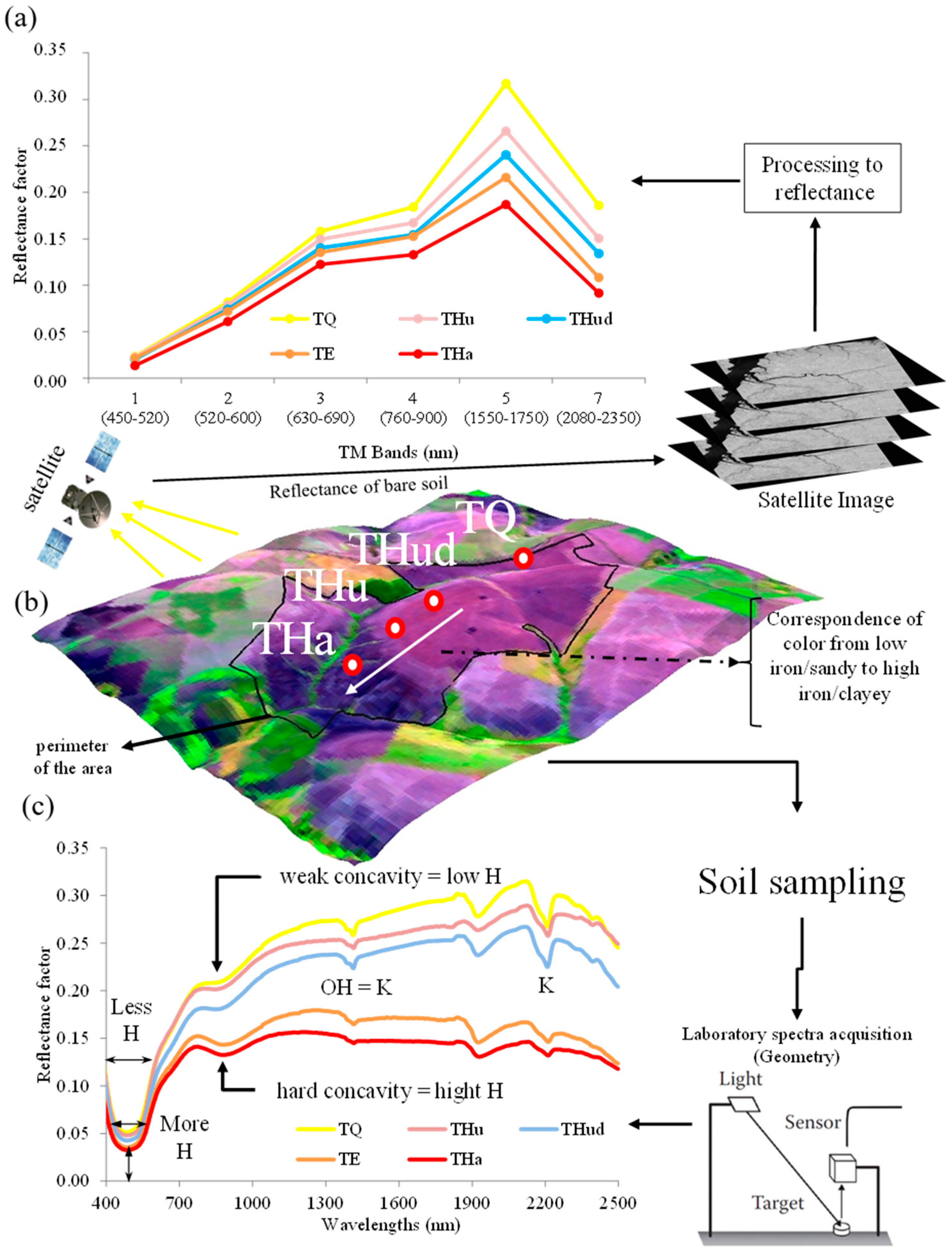[55,56] observed great differences on spectra from sandy to clayey tropical soils. In fact, spectral information shapes differ between these granulometric groups (Figure 4c). A low albedo was observed in the VIS and high in SWIR for sandy soils. On the other hand, clayey soil does not change significantly between these regions. This occurs due to the organic matter that absorbs energy in VIS, as quartz reflects in SWIR. This is a clear indication of correlation between granulometry and spectral data as determined by [57] in tropic soils. In fact, the soils have a great variation on clay content (21% to 84%, Table 1).

From laboratory to satellite data, it was observed the same tendency (Figure 4c,d). The spectrum loses the information of details on shapes because Landsat has only six bands against 1500 of the laboratory sensor. On the other hand, the aspect from VIS to NIR to SWIR on albedo shows a positive tendency with ascendant shape, in agreement with [55]. Since the SWIR spectra remained stable in laboratory measurements, the satellite data from band 5 to 7 had a slight declining tendency on absorption (Figure 4d). This behavior is due to the soil moist in field condition when the satellite sensor acquired the information. Despite this, band 5 remains remarkable on discrimination of soils with different textures, in agreement with [56].

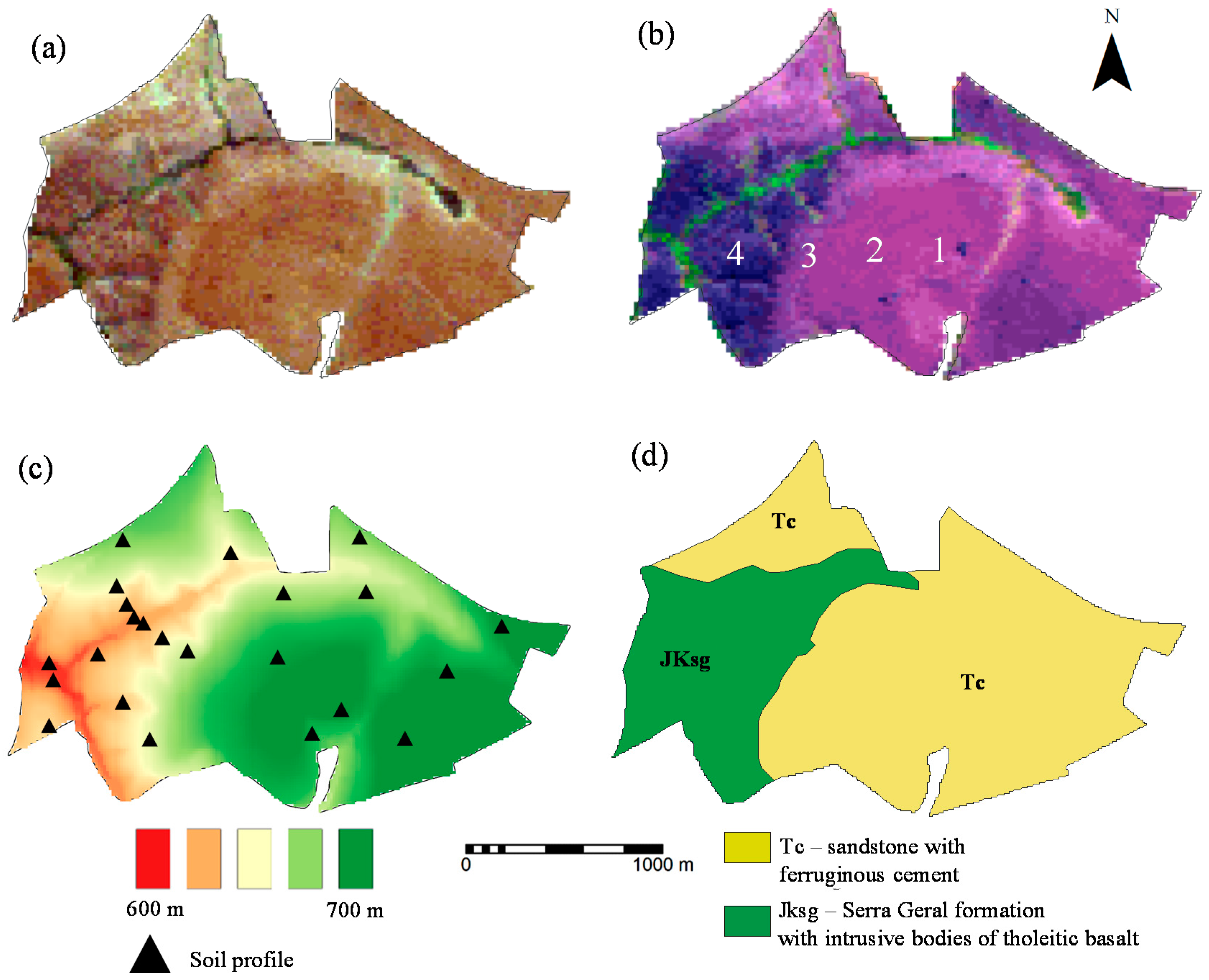
When there are high levels of iron in the soil, the Landsat image shows purple coloration in composition 543 (RGB) and brown coloration in the 321 (Figure 3a,b). The point is that the image “color” gives a clue of the soil information, but does not express a spectral pattern. That is why we should go forward to analyze punctual spectral signature. The wavelengths of iron oxides absorption are between 630 and 690, and 760 and 900 nm, corresponding, respectively, to the wavelengths of bands 3 and 4 of Landsat. Thus, with the presence of oxides, the images will be brown or purple according to the composition of the bands and the presence of the elements. Therefore, there is a great correspondence of the spectra from the top of the topossequence (sandy and low iron) to the bottom (clayey and high iron), with the color indicated in composition 5/4/3, in the sequence from point 1 to 4 (Figure 3b).

As mentioned, Figure 3a,b presents the differences on color related with the mineralogy. At the location 4 (THa2) in Figure 3b (image 543), soils with high clay and Fe₂O₃ content presents dark blue color. On the other hand, when soils have less iron content and gets more sandy (TQ, location 4 in Figure 3b), the color goes to light pink. Composition 321 indicates the real information and is in agreement with field observation.

When we analyzed the top soil spectra, differences were observed in each soil class (Figure 5a). We acquired the satellite spectra from a bare soil pixel. Then, a soil sample collected in the center of the same pixel at field was used for comparison with the laboratory spectra. We observed shape and intensity spectral alteration from laboratory to satellite data for THud and TQ (Figure 5a). Indeed, THud has high iron and clay content, but low quartz. THa is very clayey with high iron (Fe₂O₃) content, magnetite and ilmenite, which brings us to a flat spectral-shape in accordance with [57]. This tendency is observed in both laboratory and satellite data (Figure 5c,d). In convergence with spectra, color goes from weak to strong purple, as well (Figure 5b).

We saw differences between the shapes related with iron oxides (Figure 5c). At 530 nm, hematite absorbs more energy producing a wider shape, and at 850 nm, it presents a strong concavity. At 1900 nm, there is the OH-stretch of kaolinite associated with the alumina vibration in 2200 nm. These differences cannot be observed in Figure 5a because the multispectral sensor has limitation. However, the spectral intensity tendencies were similar in both satellite and laboratory sensors. Great differentiation between soils occurred at bands 5 and 7 related with quartz.

Indeed, image colors indicate soil variations. Figure 3 shows that sandy soils at top altitude has weaker color. As we go to lower altitudes, pedogenetic alteration occurs. The area at the top have soils developed from sandstone and at lower altitudes basalt. Geology map (Figure 3d) indicates these observations. Thus, the image plus top soil spectra and geology map helps on the detection of soil alteration, and perhaps soil units. On the other hand, spectra from top soil are important but cannot discriminate them accurately, because the diagnostic horizon is in undersurface (B horizon). In this case, we must change the strategy and evaluate surface and undersurface as indicated by [58], or use relief parameters strategy.

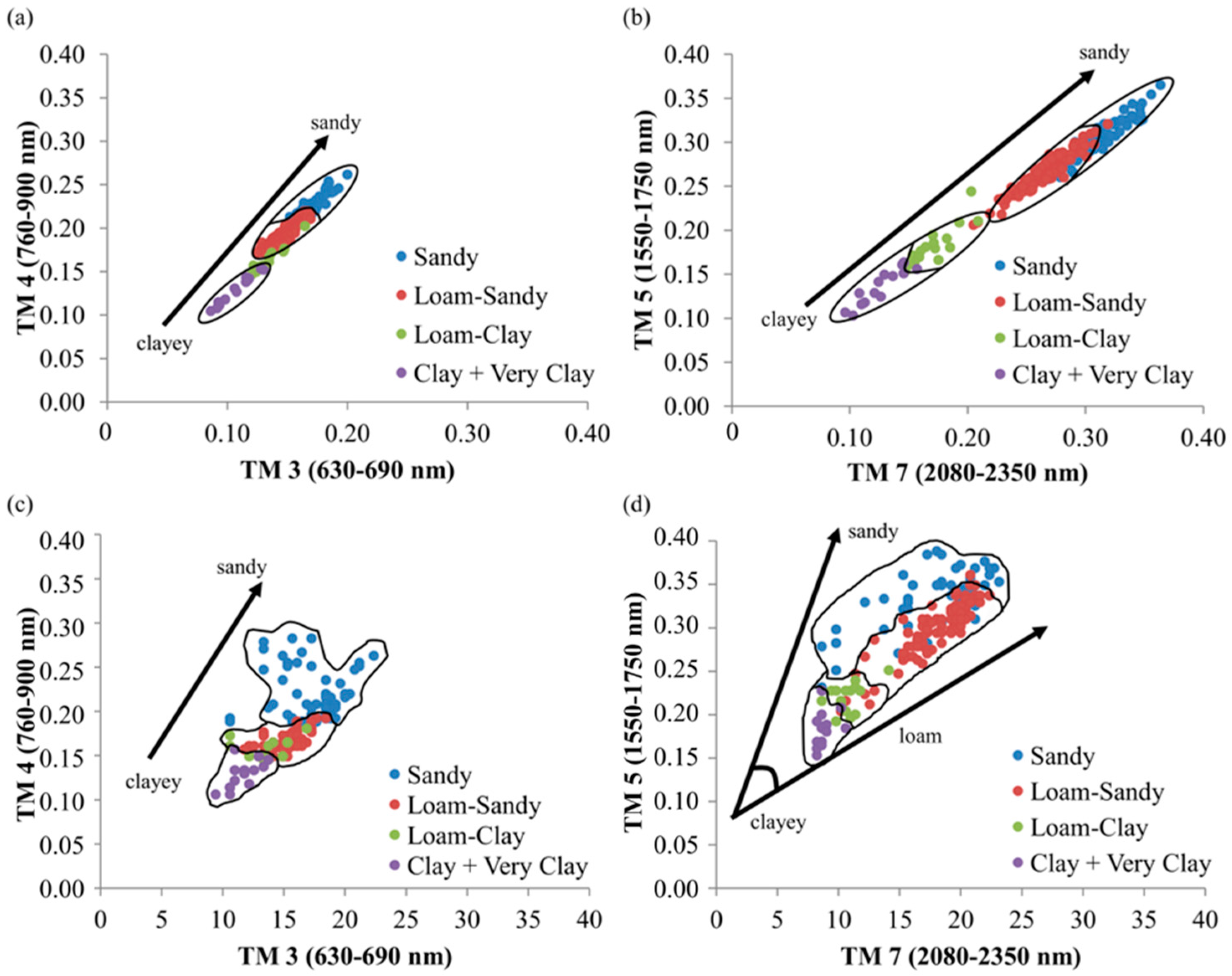
Comparison between laboratory and satellite information can also be realized by soil line concept [59]. Figure 6a indicates the relation between bands 4/3 and 5/7, where spectra are clearly close to 1:1 line since we know they are bare and dried samples, in agreement with [59]. The same occurs for band 5/7 (Figure 6b) but more dispersed along the soil line. The use of bands 5 and 7 for better discrimination of soil texture corroborates with findings [56]. When using satellite data, the quality acquisition is not always controlled at field level for some aspects, such as moist, litter, roughness and spatial distribution. These issues can be diminished by using images acquired in dry season and after plowing. Pre-processing and reflectance transformation is also necessary. Thus, soil line observations associated with the spectra indicate that satellite data were ratified by laboratory with quality control.

While in laboratory all samples are dried, bands 5 and 7 are similar on intensities and take the dispersion to 1:1 line (Figure 6). On the other hand, soil represented by satellite images is not completely dry and causes a lower reflectance intensity from band 5 to 7 [60]. This makes the plots more dispersed. The same happens with clayey soils, but with less intensity. Moisture in clayey soils affect band 7 but not band 5. Instead, band 5 is influenced by quartz. Thus, the greater dispersion out of the soil line would be for sandy soils, and the opposite for clayey ones. This is clear in Figure 6b for loam-sandy soil, where the dispersion is low for either bands 3 and 4 (Figure 6a). It was observed that sandy textures were also more dispersed. The explanations for these findings are based on mineralogy, not moisture. Sandy soils have less magnetite, ilmenite and hematite, and, therefore, show differences between these bands. Clayey soils with high Fe₂O₃ (Table 1) and magnetite does not change intensity between these bands, and thus, adjust to 1:1 line.

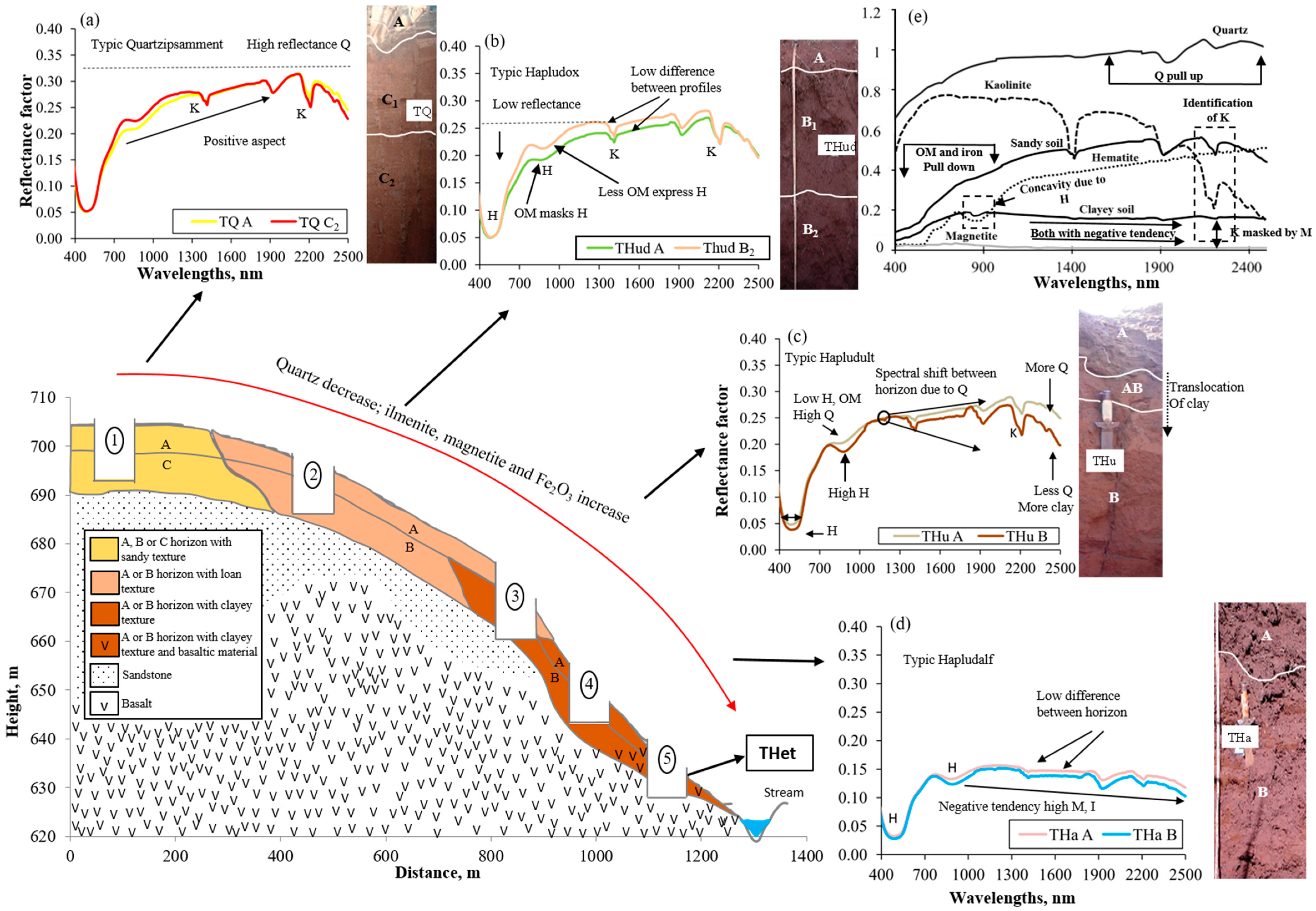
The characterization of soil classes by spectra was better verified by profile samples. Figure 7a indicates no alteration between horizons for TQ. This is true since this soil had less than 15% clay in all profile with very homogenous color. The same happened with Thud (Figure 7b), although having more clay and lower reflectance. Both soils do not have texture differences between A and B horizons, which is expressed by similar spectra. The Typic Hapludalf (Figure 7c) has its characteristics as with low reflectance in all bands, negative tendency and flat shape. This occur due to its mineralogy, developed from basalt it has high clay content, high presence of magnetite and ilmenite, dark red color and high hematite content. The magnetite “pull” the spectra to lower reflectance in SWIR, and thus have a negative tendency. A Typic Hapludult has different clay contents from A to B horizon (Table 1). This characteristic reflects on spectra (Figure 7d). Horizon A presents higher reflectance at SWIR and horizon B has lower reflectance. In fact, there is a shift between horizons in about 1200 nm, which is an indicative of the gradient texture as previously observed by [57].

Soils alter along topossequence from point 1 to 5 (Figure 7). As we start in upper altitudes, soils are mostly developed from sandstone (TQ) and are sandy. This characteristic goes all over the profile. When we go down in altitude, sandy texture starts to shift to loam and we reach the THud soils. Despite this, the texture does not change along the profile. On the other hand, on point 3, the loam texture on horizon A continues the same, but B horizon is interrupted and shifts from loam to clay. This gradient of texture creates the THu soil. The alteration occur because during weathering, clay translocated from A to B horizon. Since the parent material is also changing, as sandstone is giving place to basalt, soils starts also to be more clayey. At point 4, clay is no more translocated, but developed in-situ directly from basaltic rocks. On point 5, A horizon is still clayey, and have a B horizon (cambic horizon), with presence of rocks and primary minerals. Thus, point 5 reveals a low deep soil.

Laboratory spectral strategy has the ability to obtain information from surface and undersurface soil. This information is much more detailed since the equipment is hyperspectral, and absorption features can express soil mineralogy. The topsoil information can only be compared with satellite data if the soil is exposed. However, Landsat spectra provide soil information with low detail since it has only six bands. Despite this limitation, the spectral pattern and intensity provided similar tendency with laboratory data (Figure 6). This kind of information shows the importance of satellite spectra. On the other hand, satellite image also provides color composition (Figure 3 and Figure 5). This information showed great relationship with mineralogy and soil attributes, such as texture. Therefore, soil evaluation and spacialization presented good results when punctual spectral patterns and image composition were applied together. Moreover, laboratory data is very important to validate and understand satellite information as well.

A limitation of image spectral patterns on soil classification could be the impossibility to observe undersurface soil (diagnostic horizon). In fact, this is impossible for satellite images. An example could be the evaluation of THu, for which spectra are different between horizons (Figure 7c). In contrast, the classification of this soil presupposes the presence of texture gradient between A and B horizons. Table 1 shows that clay goes from 19.2 to 39.8 g·kg⁻¹ for this soil class. Thereby, soils with similar characteristics of A and B horizons have better chance for discrimination by satellite images, such as the THud and TQ.

The fact is that surface information of THud (Figure 6a) is expressed by a high reflectance in band 5, which is related with its low clay content. Although the texture could be identified, the soil classification could not be afforded with that single information. On the other hand, we saw that all soils were discriminated only by surface analysis. This led us to agree with [61], which obtained 70% of agreement on soil discrimination by Landsat image assisted with geological map.

Thus, despite image only detect surface layer, this information was important for soil discrimination, not classification. We can infer from the soil line, but not make a final decision of soil classes. Indeed, Zeng et al. [35] observed an agreement between different soils at field with surface satellite information using discriminant analyses. This work shows that, despite the fact that satellite image does not detect undersurface soil, surface should have a specific combination of attributes that differs between them. Nevertheless, caution must be taken because in many cases, only surface information will not be sufficient to discriminate. These first results indicated that satellite and laboratory data, used together, aggregated strong evidence on the discrimination of pedological classes. Thus, we used this knowledge for the next steps to reach the digital soil maps.

3.3. Prediciton of Soil Attrinutes by Spectra

The calibration and validation sets included a total of 103 and 102 samples from surface and undersurface layer, respectively (

Table 2. Descriptive statistics of soil attribute values of soil samples from the transect sections.

Soil Attribute	Minimum	Maximum	Mean	SD 1	Skewness
	Layer A (n = 103) 2
Fe2O3 g·kg−1	10	252	47.7	55.8	2
Al2O3 g·kg−1	15	158	49	34.6	1.9
SiO2 g·kg−1	24	156	53	29.4	2
TiO2 g·kg−1	4.8	59	14.9	14.8	1.7
Clay %	8	67	21.9	14.8	1.7
3 BS mmolc·kg−1	2.7	76.9	23.7	14.1	1.4
	Layer B (n = 102) 2
Fe2O3 g·kg−1	9	216	55.4	55.1	1.7
Al2O3 g·kg−1	25	170	72.4	38.6	1.5
SiO2 g·kg−1	32	166	71.5	32.4	1.6
TiO2 g·kg−1	5.9	56	16	13.5	1.6
Clay %	12	76	27.4	16.7	1.5
3 BS mmolc·kg−1	2.1	93.3	15.9	17	2

¹ Standard Deviation; ² Number of samples; ³ Sum of cations: Ca + Mg + K.

). The wide range of soil attributes variation is a consequence of the two completely different parent materials (basaltic rocks and sandstone) from which derived the soils (Figure 3d).

The principal component analysis was performed to reduce the collinearity between data. In the laboratory spectra dataset, the first three components were able to explain 99.4% of the spectral variation: PC1 95.64%, PC2 3.19% and PC3 0.58% (Figure 8a). It was also possible to identify a clustering between the surface and undersurface horizons. When the PCA was performed in the wet-laboratory data (Figure 8b), 78.3% of the variation was explained by the first three components. In both analyses, the clustering was due to the granulometry and organic matter content, which significantly differed in depth.

Additionally, when the PCA was performed in laboratory spectra, the soil samples acquired at toposequences were representative of the whole area. Figure 8c,d shows a homogenous distribution of the calibration and validation soil samples in the whole laboratory dataset. Thus, the spectral library used for attribute quantification was able to assist on soil classification.

For calibration models, it was necessary to transform the reflectance spectra into absorbance (log 1/R). The calibrated models used for creating the spectral library presented good capability for soil attributes quantification (

Table 3. Results of the models calibration and validation for the quantification of soil attributes.

Soil Attribute	PLS Factors	Cross Validation Within the Calibration Set (n = 155) 1				Cross Validation for Validation Set (n = 50) 1
		R2adjusted	RMSE	ME	SDE	R2adjusted	RMSE	ME	SDE
Fe2O3 g·kg−1	9	0.88	18.99	−1.11	1.12	0.85	23.02	3.28	0.65
Al2O3 g·kg−1	6	0.81	16.58	0.37	−0.38	0.77	19.05	5.28	−2.55
SiO2 g·kg−1	4	0.77	15.07	0.87	0.12	0.71	18.72	−1.94	5.02
TiO2 g·kg−1	9	0.91	4.14	−0.22	0.22	0.87	4.93	0.69	−0.32
Clay %	9	0.93	4.26	0.22	−0.22	0.90	5.07	0.53	−0.69
2 BS mmolc·kg−1	6	0.76	8.24	−0.35	0.35	0.76	6.81	−0.63	−0.03

¹ Number of samples; ² Sum of cations: Ca + Mg + K.

). We obtained high R² and low RMSE values, such as 0.9% and 5% for clay, respectively, and 0.85 and 23 g·kg⁻¹ for iron, respectively. These two variables are important for soil classification. The final dataset of the undersurface layer consisted in 422 samples, of which 155 were used for model calibration, 50 for model validation and 217 (which did not have soil routine analysis information) for soil attribute prediction. These results gives support to using spectra to optimize wet analysis on the entire area, in agreement with [32].

3.4. Spatial Modeling of Soil Attributes in Undersurface Layer

The use of VIS-NIR-SWIR spectroscopy technique allowed the acquisition of new undersurface soil information for the 217 points. In other words, the spatial resolution of the information was improved from transect sections (255 points with soil attribute information) to a grid of 100 m² (422 points with soil attribute information). The improved resolution allowed the spatial structures of soil attributes to obtain high R² and low RMSE values for kriging interpolations (

Table 4. Results of the geostatistical analysis for the soil attribute mapping in the surface layer.

Soil Attribute	Semi-Variogram Characteristics					Leave-One-out Cross Validation of Kriging Interpolations
	Model	Nugget (Co)	Sill (Co + C *)	Range (m)	C/(Co + C)	R2adjusted	RMSE	ME
Fe2O3 g·kg−1	Spherical	241.11	998.88	868.01	0.76	0.87	20.01	−0.21
Al2O3 g·kg−1	Spherical	222.95	512.78	801.24	0.57	0.78	18.58	−0.40
SiO2 g·kg−1	Spherical	102.60	205.21	895.11	0.50	0.84	10.73	0.67
TiO2 g·kg−1	Spherical	8.31	73.91	832.78	0.89	0.87	5.08	−0.03
Clay %	Spherical	17.94	89.68	801.38	0.80	0.87	5.95	−0.01
1 BS mmolc·kg−1	Spherical	7.98	90.43	898.01	0.91	0.88	5.29	0.10

¹ Sum of cations: Ca + Mg + K; * Partial sill.

). The degree of spatial dependence (evaluated by the proportion of spatial) was strong for all attributes (Table 4). All semi-variograms have a similar range between 800 and 900 m and the spatial patterns were controlled by the topography. A close relationship of soil attributes maps with elevation was observed (

Table 5. Correlation matrix of predicted soil attribute maps and land parameters.

	Al2O3	Clay	Ki	Kr	Fe2O3	SiO2	TiO2	BS 1	Elev 2	MC 3	Slope
Al2O3	1	0.99	−0.59	−0.76	0.98	0.94	0.97	0.97	−0.84	−0.01	0.37
Clay		1	−0.5	−0.70	0.99	0.97	0.98	0.98	−0.86	−0.01	0.38
Ki			1	0.93	−0.53	−0.32	−0.48	−0.41	0.29	−0.01	−0.12
Kr				1	−0.74	−0.55	−0.71	−0.64	0.51	0.00	−0.23
Fe2O3					1	0.94	0.99	0.97	−0.85	−0.01	0.38
SiO2						1	0.96	0.98	−0.90	−0.02	0.42
TiO2							1	0.98	−0.88	−0.02	0.41
BS								1	−0.89	−0.02	0.42
Elev.									1	0.09	−0.55
MC										1	0.00
Slope											1

¹ Sum of cations: Ca + Mg + K; ² Elev.: Elevation; ³ MC: Mean curvature.

). This is consistent with several studies where soils derived from basalt, where the spatial variability of their attributes is partly controlled by topographic position, especially in the tropics [62].

3.5. Removing the Redundancy on the Datasets (DsSA, DsSB and DsTP)

The high degree of correlation observed between the predicted soil attributes maps (Table 5) indicates redundant information that could be summarized. Thus, all soil attribute maps were reduced through the PCA to one map (DsSA-PC1) that explained 97.9% of the total variance found. In the same way, the seven bands of the satellite image were reduced by PCA to one band (IPC1) that accounted for 91% of the total variance. Only the new first band (DsSB-PC1) was considered since this represents a large part of the albedo which in turn is related to tropical soil texture [57,63]. Usually, the first PC (in this case DsSB-PC1) of the Landsat TM images bands explain over 80% of the total variance. In this way, the final input variables or features used to create the classification rules and for the supervised classification were DsSA-PC1, DsSB-PC1, elevation, mean curvature and slope. The quantity and quality of information related to soil and landscape favored the soil classification. However, much of this information could be redundant. In this way, the digital soil mapper must extract only the most important information. In this case, five from a set of 17 initial variables were used directly for the supervised classification.

As observed, elevation had great correlation (r = −0.85) with iron. Thus, high altitudes presented lower iron. In fact, images indicate light color in those areas, with soils developed by sandstone (Figure 3 and Figure 4). The same occurred for clay (r = −0.86), which agrees with field observation where we had sandy soils at top relief and clayey at bottom. We also observed chemical information (Sum of cations, BS), which had a great correlation (r = −0.89) with the elevation (Elev.). Indeed, soils at top (TQ) and bottom (THa) have poor and high fertility, respectively. Thus, although spectra have low sensitivity for chemical quantification, relief parameter contributed to detect these characteristics.

3.6. Soil Attributes Spacialization and Its Relationship with Soil Classification and Mapping

Clay and Fe₂O₃ are important attributes on soil classification. As the estimative of soil attributes got important performance (and was corroborated by literature), we present their spatial distribution, both determined by laboratory compared with spectroscopy (Figure 9). We observe a very close relationship between them. We observe sandy soils at top altitudes, going to loam in middle and clayey in bottom in horizon A (Figure 9a,b). As we can observe in horizon B, in top altitudes (Figure 9c,d), we have sandy texture in undersurface, what characterizes the TQ. As we go down in altitude difference becomes greater because of the variance in texture, which is related with parent material (Figure 7).

Iron is an important attribute for soil classification, as observed from B horizon. Figure 9g,h, indicate the amount of this attribute in B horizon. Observe that the amount goes from low (9 g·kg⁻¹) to high (215 g·kg⁻¹) on the sequence high to low altitudes. This occurs because altitude is related with parent material (Basaltic rocks). Despite satellite images do not reach undersurface data, surface information can give important indication. Figure 9f shows clear differences between this attribute along the area, and can also be related with image composition 5R4G3B (Figure 3b). Area goes from pink to dark blue color (high to low altitudes). Thus, sensing from images gave important “clue” on where could have soils alteration. These “clues” were important to choose areas with soil alteration as done in this work.

3.7. Supervised Classification and Digital Soil Maps

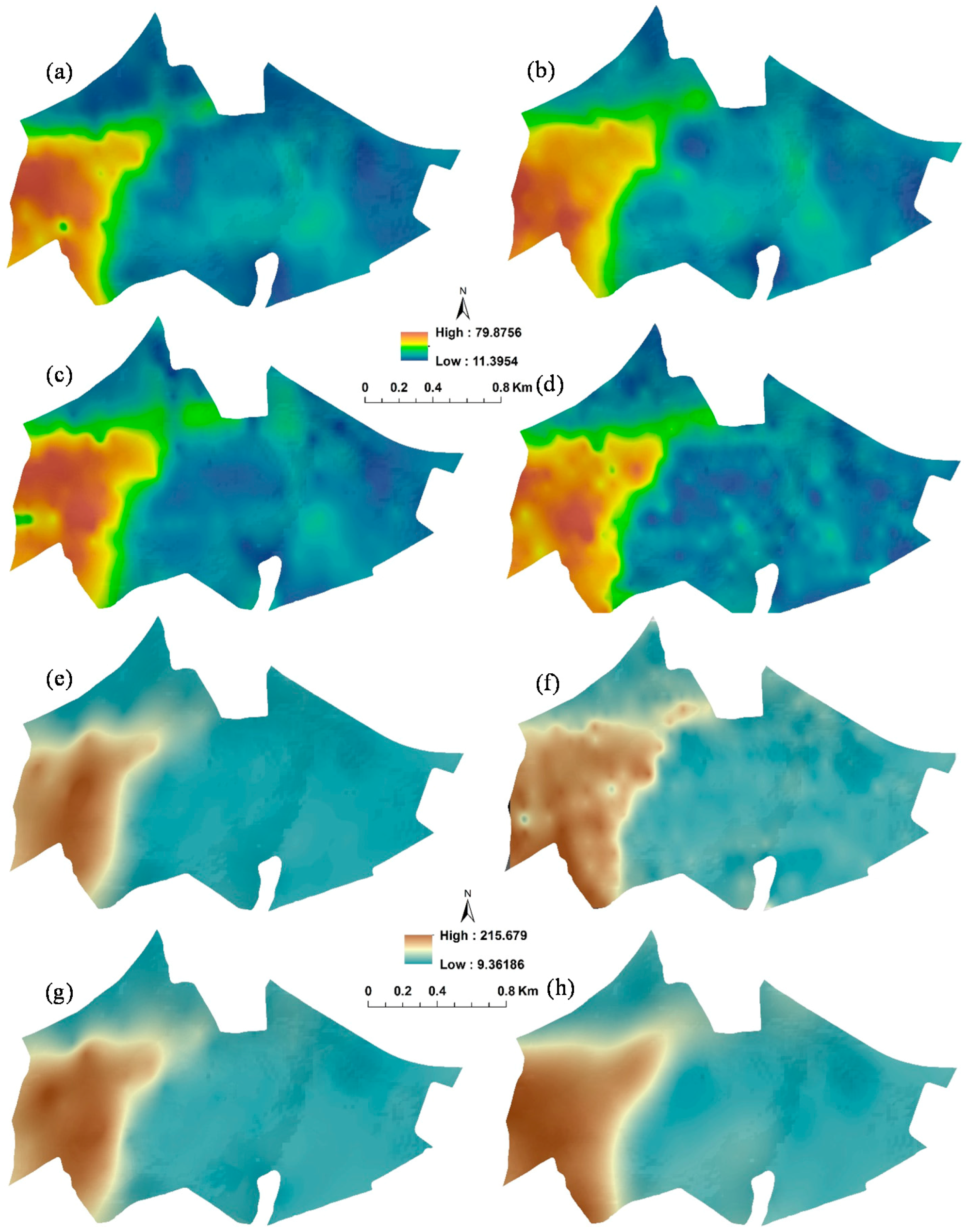
Supervised classification of the DsSA-PC1, DsSB-PC1 and DEM parameters resulted in two soil maps. For the digital TFS-1 map (Figure 4e), a kappa index (κ) of 0.52 and overall accuracy of 69% were obtained. The TFS-2 map (Figure 4f) obtained κ = 0.45 and an overall accuracy of 62%. These results corresponded to a good performance [54].

The degree of spatial correspondence (DSC) between the digital and traditional TFS-1 maps for each soil class showed similar values with the Sc (

Table 6. Degree of Spatial Correspondence (DSC) between the respective soil classes of the conventional and digital soil maps.

DSC
TFS-1	%	TFS-2	%
Typic Hapludox	76.5	Typic Hapludox I	73.9
Typic Hapludult	76.1	Typic Hapludox II	40.0
Typic Quartzipsamment	37.8	Typic Hapludult I	66.4
Typic Hapludalf	54.9	Typic Hapludult II	48.2
Typic Eutrudepts	32.8	Typic Quartzipsamment	42.5
		Typic Hapludalf I	0.0
		Typic Hapludalf II	36.3
		Typic Eutrudepts I	25.1
		Typic Eutrudepts II	0.0

TFS-1: Traditional soil map with order and suborder classification; TFS-2: Traditional soil map with order and suborder classification, plus other information (texture, color and fertility).

and

Table 7. Percentage of the each traditional soil class area covered by each digital soil class area (Sc) for the TFS-1 maps.

		Traditional Map
		THud	THu	TQ	THa	TE
Digital map	THud	76.5	19.2	35.3	0	10.8
	THu	11.0	76.0	26.9	23.7	32.8
	TQ	9.7	0.1	37.8	0	0
	THa	2.5	3.8	0	54.8	23.6
	TE	0.3	0.1	0	21.5	32.8

THud: Typic Hapludox; THu: Typic Hapludult; TQ: Typic Quartzipsamment; THa: Typic Hapludalf; TE: Typic Eutrudepts.

). According to the DSC, Typic Hapludox, Typic Hapludult and Typic Hapludalf were the soils that presented good agreement between the digital and traditional assessments. Typic Quartzipsamment and Typic Eutrudepts showed low values of spatial correspondence.

Most of the soil classes of the TFS-1 and TFS-2 digital maps showed relatively low levels of discrepancies with their correspondent traditional soil class maps. Therefore, the similarity with field maps was high (Figure 4). The predicted Typic Hapludox covered some areas of the traditional Typic Quartzipsamment. This is related to the clay fraction of the Typic Hapludox, which was lower than 20%. In this case, these soil classes had similar clay content. This discrepancy was expected, since Typic Hapludox and Typic Quartzipsamment occur in similar relief compartments.

Concerning the discrepancies between Typic Hapludult in areas of Typic Hapludalf of the soil traditional map, which showed a Sc = 23.7 (Table 7), the chemical attributes could not allow the discrimination between them. Thus, the weight of the PC for soil attributes estimated in the undersurface layer was low because it did not provide sufficient information for the discrimination of these soil classes. With the surface satellite image, it is possible that their differentiation was less complex. However, since these soils have different texture between surface and undersurface, the discrimination remains complicated even sometimes by using the traditional method. On the other hand, most of the classification discrepancies between TFS-2 digital map and its correspondent soil traditional map occurred between subgroups of the same soil class (

Table 8. Percentage of the each traditional soil class area covered by each predicted soil class area (Sc) for the TFS-2 maps.

		Traditional Map
		THud-I	THud-II	THu-I	THu-II	TQ	THa-I	THa-II	TE-I	TE-II
Digital map	THud-I	73.7	35.8	21.0	20.9	42.9	0	0	17.3	0
	THud-II	4.1	31.6	0	0	0	0	0	0	0
	THu-I	6.2	25.3	76.3	46.6	12.2	20.8	49.2	42.1	99.2
	THu-II	0.1	0	0.2	32.5	0	0	0	0	0
	TQ	13.5	2.5	0.2	0	44.9	0	0	0	0
	THa-I	0	0	0	0	0	0	0	0	0
	THa-II	1.4	4.8	2.1	0	0	44.5	39.4	0	0
	TE-I	1.1	0	0.1	0	0	34.7	11.4	33.7	0.8
	TE-II	0	0	0	0	0	0	0	7.0	0

THud-I: Typic Hapludox I; THud-II: Typic Hapludox II; THu-I: Typic Hapludult I; THu-II: Typic Hapludult II; TQ: Typic Quartzipsamment; THa-I: Typic Hapludalf I; THa-II: Typic Hapludalf II; TE-I: Typic Eutrudepts I; TE-II: Typic Eutrudepts II.

).

Finally, the purity of the conventional and traditional soil maps could have affected the purity of the digital soil map. For instance, Beckett et al. [64] found a range of mapping purity between 65% and 86% for a conventional soil survey at 1:25,000 scale. Therefore, errors in traditional soil maps could interfere in the creation of the training and prediction rules, decreasing the performance of the digital technique. On the other hand, we can infer that the purity of digital soil maps could be closer to the conventional approach ranges mentioned before, if we take into account the overall accuracy indexes found in this work.

Indeed, other authors have obtained variation in the quality indicators when they attempted to develop a digital soil map. There is an indication that the results vary according to some parameters such as prediction co-variables, the scale, the complexity of the area and the statistical methods [9,65]. Although [34] have reached 91% of agreement for Oxisol class in their study, Alfisol and Ultisol classes just reached 46% of concordance between conventional and digital maps. The study was carried out in a very complex area with heterogeneous soils, in a semidetailed scale level (1:50,000), using hyperspectral data, Landsat images and stream density as prediction variables.

The area mapped in the current paper reached good results (mean of 69%) regarding DSM approach with remote and proximal sensing, and with relief parameters. Arruda et al. [65] used the same area as well the information to extrapolate by pedrotransference neural net systems the entire area, reaching 75% agreement. Their results converge to the importance of DSM. Thus, the strategy to make a pedological map can vary, depending on the tools you have available and the final objective.

Bazaglia Filho et al. [9] also reached a range from 12% to 35% agreement between the traditional and digital soil map in an area of tropical soils. In that occasion, only terrain attributes derived from relif were used for soil classes prediction. The authors used a neural net system, and the bad prediction power was associated with the geological complexity of the area and the scale level of mapping (ultra-detailed map with 1:5000 scale). Nanni et al. [66] used laboratory and orbital spectra looking towards pedological mapping. Demattê et al. [67] used spectroscopy and relief variables to reach very good similarity with the traditional map. In fact, this was also indicated by [68] when using aerial photographs in addition with field spectroscopy. These papers corroborates with [69] for whom DSM can support the production of functional maps. These studies are also in agreement with the present work, where a good performance (69%) between the digital and traditional map was reached. It is also important to state that satellite images (specifically of Landsat) can be obtained free on the Internet. Regardless, the image must be taken in the same time of soil sampling, with clear sky and good climate, processed and transformed into reflectance, and with complete bare soil, Thus, the variations of quality seems to be a matter of the objective of the user (e.g., scale), and mainly, on how user develops the strategy to map the soil.

4. Conclusions

• Soil laboratory spectra is strong information to validate and understand satellite data.
• Spectral reflectance with local models indicated high performance for clay, iron and weathering indexes with R² from 0.76 to 0.90. This corroborates the hypothesis for quantification of soil attributes all over the area, getting more spatial representativeness without wet laboratory analysis. It was used near 155 samples to model the other 317, allowing us a high observation density. On the other hand, chemical information (such as the sum of cations) could not be quantified by spectra. On this matter, we changed the strategy and used elevation to assist the soil mapping, which had a good correlation with the sum of bases (r = −0,85).
• The predicted information improved the spatial resolution of soil mapping. This facilitated the identification of spatial structures of soil attributes obtaining good predictions with 0.78 until 0.88 R². Good prediction performances are important because the final digital soil class maps depends on: (a) the errors of the predictions made by the calibration spectral models; and (b) the errors resulting from the spatial interpolation process. Therefore, these errors can be incorporated into the algorithm used for digital soil mapping.
• Soils with homogenous spectra from horizon A to B, such as Oxisols, can be detected by satellite data, contrary to Ultisols and Alfisols. On the other hand, relief parameter such as elevation was able to discriminate these soil classes, and aggregated with spectra information.
• Satellite (surface) and laboratory (surface and undersurface) spectral information, and relief parameters, when integrated, have strong potential for discriminating pedological soil classes.
• The key of this work was to obtain pattern samples along topossequences constructing a database (library) of spectra, which assisted quantification of attributes for all the area, and corroborate with the satellite information.
• Color compositions 5R4G3B from Landsat have great performance on discriminate soils developed from sandstone and basalt. From sandy (low iron) to clayey (high iron) topossequence, the colors went from weak/light purple to strong blue, respectively. Thus, color and spectral patterns signatures can evaluate satellite data to achieve soil information.
• In some situations, spectra give information that relief does not. The opposite is also true. Images help on delineation giving information about the surface, but not for the undersurface soils. Thus, the integration of soil spectroscopy information using laboratory and satellite spectral libraries, terrain parameters and statistical methodologies allowed the prediction of a detailed pedological map. The predictive performance of the methodology for digital soil class mapping was satisfactory. Digital soil maps were similar to the conventional ones showing a kappa index of 0.52 and global accuracy of 69%, as a field validation of 75%–80%.

References

1. Mendonça-Santos, M.L.; dos Santos, H.G. The state of the art of Brazilian soil mapping and prospects for digital soil mapping. Dev. Soil Sci. 2006, 31, 39–54. [Google Scholar]
2. Santos, H.G.; Hochmüller, D.P.; Cavalcanti, A.C.; Rêgo, R.S.; Ker, J.C.; Panoso, L.A.; Amaral, J.A.M. Procedimentos Normativos de Levantamentos Pedológicos; EMBRAPA-SPI; EMBRAPA-CNPS: Brasília; Rio de Janeiro, Brasil, 1995. [Google Scholar]
3. Minasny, B.; McBratney, A.B. Digital soil mapping: A brief history and some lessons. Geoderma 2016, 264, 301–311. [Google Scholar] [CrossRef]
4. Coleman, T.L.; Agbu, P.A.; Montgomery, O.L.; Gao, T.; Prasad, S. Spectral band selection for quantifying selected properties in highly weathered soils. Soil Sci. 1991, 151, 355–361. [Google Scholar] [CrossRef]
5. Viscarra Rossel, R.A.; Walvoort, D.J.J.; McBratney, A.B.; Janik, L.J.; Skjemstad, J.O. Visible, near infrared, mid infrared or combined diffuse reflectance spectroscopy for simultaneous assessment of various soil properties. Geoderma 2006, 131, 59–75. [Google Scholar] [CrossRef]
6. Lagacherie, P.; McBratney, A.B.; Voltz, M. Digital Soil Mapping: An Introductory Perspective; Elsevier Science: Amsterdam, The Netherlands, 2006. [Google Scholar]
7. Hartemink, A.E.; Minasny, B. Towards digital soil morphometrics. Geoderma 2014, 230–231, 305–317. [Google Scholar] [CrossRef]
8. Legros, J.-P. Mapping of the Soil; Science Publishers: Enfield, Jersey, Plymouth, 2006. [Google Scholar]
9. Bazaglia Filho, O.; Rizzo, R.; Lepsch, I.F.; Prado, H.; Gomes, F.H.; Mazza, J.A.; Demattê, J.A.M. Comparison between detailed digital and conventional soil maps of an area with complex geology. Rev. Bras. Ciênc. Solo 2013, 37, 1136–1148. [Google Scholar] [CrossRef]
10. Ziadat, F.M.; Taylor, J.C.; Brewer, T.R. Merging Landsat TM imagery with topographic data to aid soil mapping in the Badia region of Jordan. J. Arid Environ. 2003, 54, 527–541. [Google Scholar] [CrossRef]
11. Ziadat, F.M. Land suitability classification using different sources of information: Soil maps and predicted soil attributes in Jordan. Geoderma 2007, 140, 73–80. [Google Scholar] [CrossRef]
12. Dobos, E.; Micheli, E.; Baumgardner, M.F.; Biehl, L.; Helt, T. Use of combined digital elevation model and satellite radiometric data for regional soil mapping. Geoderma 2000, 97, 367–391. [Google Scholar] [CrossRef]
13. Dobos, E.; Montanarella, L.; Nègre, T.; Micheli, E. A regional scale soil mapping approach using integrated AVHRR and DEM data. Int. J. Appl. Earth Obs. Geoinf. 2001, 3, 30–42. [Google Scholar] [CrossRef]
14. McBratney, A.B.; Santos, M.L.M.; Minasny, B. On digital soil mapping. Geoderma 2003, 117, 3–52. [Google Scholar] [CrossRef]
15. McBratney, A.B.; Minasny, B.; Viscarra Rossel, R. Spectral soil analysis and inference systems: A powerful combination for solving the soil data crisis. Geoderma 2006, 136, 272–278. [Google Scholar] [CrossRef]
16. Carré, F.; McBratney, A.B.; Minasny, B. Estimation and potential improvement of the quality of legacy soil samples for digital soil mapping. Geoderma 2007, 141, 1–14. [Google Scholar] [CrossRef]
17. Hengl, T.; Toomanian, N.; Reuter, H.I.; Malakouti, M.J. Methods to interpolate soil categorical variables from profile observations: Lessons from Iran. Geoderma 2007, 140, 417–427. [Google Scholar] [CrossRef]
18. Mora-Vallejo, A.; Claessens, L.; Stoorvogel, J.; Heuvelink, G.B.M. Small scale digital soil mapping in Southeastern Kenya. CATENA 2008, 76, 44–53. [Google Scholar] [CrossRef]
19. Demattê, J.A.; Campos, R.C.; Alves, M.C.; Fiorio, P.R.; Nanni, M.R. Visible–NIR reflectance: A new approach on soil evaluation. Geoderma 2004, 121, 95–112. [Google Scholar] [CrossRef]
20. Ben-Dor, E. Quantitative remote sensing of soil properties. Adv. Agron. 2002, 75, 173–243. [Google Scholar]
21. Shepherd, K.D.; Walsh, M.G. Development of reflectance spectral libraries for characterization of soil properties. Soil Sci. Soc. Am. J. 2002, 66, 988–998. [Google Scholar] [CrossRef]
22. Vasques, G.M.; Demattê, J.A.M.; Viscarra Rossel, R.A.; Ramírez-López, L.; Terra, F.S. Soil classification using visible/near-infrared diffuse reflectance spectra from multiple depths. Geoderma 2014, 223–225, 73–78. [Google Scholar] [CrossRef]
23. Shi, Z.; Ji, W.; Viscarra Rossel, R.A.; Chen, S.; Zhou, Y. Prediction of soil organic matter using a spatially constrained local partial least squares regression and the Chinese vis-NIR spectral library. Eur. J. Soil Sci. 2015, 66, 679–687. [Google Scholar] [CrossRef]
24. Rizzo, R.; Demattê, J.A.M.; Lepsch, I.F.; Gallo, B.C.; Fongaro, C.T. Digital soil mapping at local scale using a multi-depth VIS–NIR spectral library and terrain attributes. Geoderma 2016, 274, 18–27. [Google Scholar] [CrossRef]
25. Bellinaso, H.; Demattê, J.A.M.; Romeiro, S.A. Soil spectral library and its use in soil classification. Rev. Bras. Ciênc. Solo 2010, 34, 861–870. [Google Scholar] [CrossRef] [Green Version]
26. Franceschini, M.H.D.; Demattê, J.A.M.; da Silva Terra, F.; Vicente, L.E.; Bartholomeus, H.; de Souza Filho, C.R. Prediction of soil properties using imaging spectroscopy: Considering fractional vegetation cover to improve accuracy. Int. J. Appl. Earth Obs. Geoinf. 2015, 38, 358–370. [Google Scholar] [CrossRef]
27. Dewitte, O.; Jones, A.; Elbelrhiti, H.; Horion, S.; Montanarella, L. Satellite remote sensing for soil mapping in Africa: An overview. Prog. Phys. Geogr. 2012, 36, 514–538. [Google Scholar] [CrossRef]
28. Debella-Gilo, M.; Etzelmüller, B. Spatial prediction of soil classes using digital terrain analysis and multinomial logistic regression modeling integrated in GIS: Examples from Vestfold County, Norway. CATENA 2009, 77, 8–18. [Google Scholar] [CrossRef]
29. Frazier, B.E.; Cheng, Y. Remote sensing of soils in the Eastern Palouse region with landsat thematic mapper. Remote Sens. Environ. 1989, 28, 317–325. [Google Scholar] [CrossRef]
30. Mulders, M.A.; Girard, M.C. Remote sensing of soils in warm arid and semi-arid lands. Remote Sens. Rev. 1993, 7, 341–363. [Google Scholar] [CrossRef]
31. Madeira, J.; Bedidi, A.; Cervelle, B.; Pouget, M.; Flay, N. Visible spectrometric indices of hematite (Hm) and goethite (Gt) content in lateritic soils: The application of a Thematic Mapper (TM) image for soil-mapping in Brasilia, Brazil. Int. J. Remote Sens. 1997, 18, 2835–2852. [Google Scholar] [CrossRef]
32. Nocita, M.; Stevens, A.; van Wesemael, B.; Aitkenhead, M.; Bachmann, M.; Barthès, B.; Ben Dor, E.; Brown, D.J.; Clairotte, M.; Csorba, A.; et al. Soil spectroscopy: an alternative to wet chemistry for soil monitoring. Adv. Agron. 2015, 132, 139–159. [Google Scholar]
33. Rizzo, R.; Demattê, J.A.M.; Terra, F.S. Using numerical classification of profiles based on Vis-NIR spectra to distinguish soils from the Piracicaba Region, Brazil. Rev. Bras. Ciênc. Solo 2014, 38, 372–385. [Google Scholar] [CrossRef]
34. Vasques, G.M.; Demattê, J.A.M.; Viscarra Rossel, R.A.; Ramírez López, L.; Terra, F.S.; Rizzo, R.; De Souza Filho, C.R. Integrating geospatial and multi-depth laboratory spectral data for mapping soil classes in a geologically complex area in southeastern Brazil. Eur. J. Soil Sci. 2015, 66, 767–779. [Google Scholar] [CrossRef]
35. Zeng, R.; Zhang, G.-L.; Li, D.-C.; Rossiter, D.G.; Zhao, Y.-G. How Well Can VNIR Spectroscopy Distinguish Soil Classes? Available online: http://www.sciencedirect.com/science/article/pii/S1537511015304001 (accessed on 29 September 2016).
36. Lepsch, I.F. As necessidades de efetuarmos levantamentos pedológicos detalhados no Brasil e de estabelecermos as séries de solos. Rev. Tamoios 2013, 9, 3–15. [Google Scholar] [CrossRef]
37. Peel, M.C.; Finlayson, B.L.; McMahon, T.A. Updated world map of the Köppen-Geiger climate classification. Hydrol. Earth Syst. Sci. 2007, 11, 1633–1644. [Google Scholar] [CrossRef]
38. Instituto de Pesquisas Tecnológicas. Mapa Geomorfológico do Estado de São Paulo; IPT: Pennsylvania, PA, USA, 1981. [Google Scholar]
39. Raij, B.V.; Andrade, J.C.; Cantarella, H.; Quaggio, J.A. Análise Química Para Avaliação de Solos Tropicais; IAC: Campinas, Brazil, 2001. [Google Scholar]
40. Klute, A.; Gee, G.W.; Bauder, J.W. Particle-size Analysis. In Methods of Soil Analisys: Part 1—Physical and Mineralogical Methods, SSSA Book Ser. 5.1; Klute, A., Ed.; SSSA, ASA: Madison, WI, USA, 1986; pp. 383–411. [Google Scholar]
41. Camargo, O.A.; Moniz, A.C.; Jorge, J.A.; Valadares, J.M.A.S. Métodos de Análise Química, Mineralógica e Física de Solos do Instituto Agronômico de Campinas; Boletim té.: Campinas, Brazil, 2009. [Google Scholar]
42. Santos, H.G.; Jacomine, P.K.T.; Anjos, L.H.C.; Oliveira, V.A.; Lumbreras, J.F.; Coelho, M.R.; Almeida, J.A.; Cunha, T.J.F.; Oliveira, J.B. Sistema Brasileiro de Classificação de Solos; 3 rev. amp.; Embrapa: Brasília, Brazil, 2013. [Google Scholar]
43. Soil Survey Staff. Soil Taxonomy: A Basic System of Soil Classification for Making and Interpreting Soil Surveys, 2nd ed.Natural Resources Conservation Service, U.S. Department of Agriculture Handbook: Washington, DC, USA, 1999.
44. Vermote, E.F.; Tanre, D.; Deuze, J.L.; Herman, M.; Morcette, J.-J. Second simulation of the satellite signal in the solar spectrum, 6S: An overview. IEEE Trans. Geosci. Remote Sens. 1997, 35, 675–686. [Google Scholar] [CrossRef]
45. Hengl, T.; Gruber, S.; Shrestha, D.P. Reduction of errors in digital terrain parameters used in soil-landscape modelling. Int. J. Appl. Earth Obs. Geoinf. 2004, 5, 97–112. [Google Scholar] [CrossRef]
46. Demattê, J.A.M.; Garcia, G.J. Avaliação de atributos de Latossolo Bruno e de Terra Bruna Estruturada da região de Guarapuava, Paraná, por meio de sua energia refletida. Rev. Bras. Ciênc. Solo 1999, 23, 343–355. [Google Scholar] [CrossRef]
47. Minasny, B.; McBratney, A.B. A conditioned Latin hypercube method for sampling in the presence of ancillary information. Comput. Geosci. 2006, 32, 1378–1388. [Google Scholar] [CrossRef]
48. Viscarra Rossel, R.A. ParLeS: Software for chemometric analysis of spectroscopic data. Chemom. Intell. Lab. Syst. 2008, 90, 72–83. [Google Scholar] [CrossRef]
49. Rossel, R.A.V.; Jeon, Y.S.; Odeh, I.O.A.; McBratney, A.B. Using a legacy soil sample to develop a mid-IR spectral library. Aust. J. Soil Res. 2008, 46, 1–16. [Google Scholar] [CrossRef]
50. Fernández Pierna, J.A.; Dardenne, P. Soil parameter quantification by NIRS as a Chemometric challenge at “Chimiométrie 2006”. Chemom. Intell. Lab. Syst. 2008, 91, 94–98. [Google Scholar] [CrossRef]
51. Ribeiro Junior, P.J.; Diggle, P.J. GeoR: A package for geostatistical analysis. R News 2001, 1, 15–18. [Google Scholar]
52. Liu, J.; Pattey, E.; Nolin, M.C.; Miller, J.R.; Ka, O. Mapping within-field soil drainage using remote sensing, DEM and apparent soil electrical conductivity. Geoderma 2008, 143, 261–272. [Google Scholar] [CrossRef]
53. Foody, G.M. Thematic map comparison. Photogramm. Eng. Remote Sens. 2004, 70, 627–633. [Google Scholar] [CrossRef]
54. Landis, J.R.; Koch, G.G. An application of hierarchical kappa-type statistics in the assessment of majority agreement among multiple observers. Biometrics 1977, 33, 363–374. [Google Scholar] [CrossRef] [PubMed]
55. Ben-Dor, E.; Chabrillat, S.; Demattê, J.A.M.; Taylor, G.R.; Hill, J.; Whiting, M.L.; Sommer, S. Using imaging spectroscopy to study soil properties. Remote Sens. Environ. 2009, 113, S38–S55. [Google Scholar] [CrossRef]
56. Madeira Netto, J.D.S. Spectral reflectance properties of soils. Photo Interpret. 1996, 34, 59–76. [Google Scholar]
57. Demattê, J.A.M.; Bellinaso, H.; Romero, D.J.; Fongaro, C.T. Morphological Interpretation of Reflectance Spectrum (MIRS) using libraries looking towards soil classification. Sci. Agric. 2014, 71, 509–520. [Google Scholar] [CrossRef]
58. Nanni, M.R.; Demattê, J.A.M.; Fiorio, P.R. Análise discriminante dos solos por meio da resposta espectral no nível terrestre. Pesqui. Agropecu. Bras. 2004, 39, 995–1006. [Google Scholar] [CrossRef]
59. Nanni, M.R.; Demattê, J.A.M. Comportamento da linha do solo obtida por espectrorradiometria laboratorial para diferentes classes de solo. Rev. Bras. Ciênc. Solo 2006, 30, 1031–1038. [Google Scholar] [CrossRef]
60. Whiting, M.L.; Li, L.; Ustin, S.L. Predicting water content using Gaussian model on soil spectra. Remote Sens. Environ. 2004, 89, 535–552. [Google Scholar] [CrossRef]
61. Nanni, M.R.; Demattê, J.A.M.; Chicati, M.L.; Fiorio, P.R.; Cézar, E.; Oliveira, R.B. Soil surface spectral data from Landsat imagery for soil class discrimination. Acta Sci. Agron. 2012, 34, 103–112. [Google Scholar] [CrossRef]
62. Thanachit, S.; Suddhiprakarn, A.; Kheoruenromne, I.; Gilkes, R.J. The geochemistry of soils on a catena on basalt at Khon Buri, northeast Thailand. Geoderma 2006, 135, 81–96. [Google Scholar] [CrossRef]
63. Saldanha, D.L.; Lima E Cunha, M.C.; Haertel, V. Spectral analysis of soils from mafic/ultramafic rocks of Cerro Mantiqueira, south-west of Rio Grande do Sul, Brazil. Int. J. Remote Sens. 2004, 25, 4381–4393. [Google Scholar] [CrossRef]
64. Beckett, P.H.T.; Burrough, P.A. The relation between cost and utility in soil survey. J. Soil Sci. 1971, 22, 466–480. [Google Scholar] [CrossRef]
65. Arruda, G.P.D.; Demattê, J.A.M.; Chagas, C.D.S.; Fiorio, P.R.; Souza, A.B.E.; Fongaro, C.T. Digital soil mapping using reference area and artificial neural networks. Sci. Agric. 2016, 73, 266–273. [Google Scholar] [CrossRef]
66. Nanni, M.R.; Dematte, J.A.M.; Junior, C.A.D.S.; Romagnoli, F.; Silva, A.A.D.; Cezar, E.; Gasparotto, A.D.C. Soil Mapping by laboratory and orbital spectral sensing compared with a traditional method in a detailed level. J. Agron. 2014, 13, 100–109. [Google Scholar]
67. Demattê, J.A.M.; Genú, A.M.; Fiorio, P.R.; Ortiz, J.L.; Mazza, J.A.; Leonardo, H.C.L. Comparação entre mapas de solos obtidos por sensoriamento remoto espectral e pelo método convencional. Pesqui. Agropecu. Bras. 2004, 39, 1219–1229. [Google Scholar] [CrossRef]
68. Cerri, C.E.P.; Demattê, J.A.M.; Ballester, M.V.R.; Martinelli, L.A.; Victoria, R.L.; Roose, E. GIS erosion risk assessment of the Piracicaba River Basin, southeastern Brazil. Mapp. Sci. Remote Sens. 2013, 38, 157–171. [Google Scholar]
69. Dobos, E.; Carré, F.; Hengl, T.; Reuter, H.I.; Tóth, G. Digital Soil Mapping as a Support for Production of Functional Maps, 1st ed.; Official Publications of the European Communities: Luxembourg, 2006. [Google Scholar]
Figure 1. Location of the study area with calibration, validation and prediction sample location.
Remotesensing 08 00826 g001
Figure 2. Illustration of the digital soil mapping strategy.
Remotesensing 08 00826 g002
Figure 3. (a) Landsat image in true color composite (3R2G1B) with bare soil; (b) color composition 5R4G3B; (c) altitude map with soil profiles indication; and (d) geology map of the area [38].
Remotesensing 08 00826 g003
Figure 4. Soil class maps: (a) TFS-1 (traditional soil map until suborder classification); (b) TFS-2 (traditional soil map until suborder classification, with additional characteristics); (c) average of spectral curve obtained in laboratory for samples with different textures; (d) spectral curve from pixels of Landsat bands; (e) digital soil map equivalent to TFS-1; and (f) digital soil map equivalent to TFS-2. K: kaolinite; G: gibbsite; Go: goethite; Q: quartz; OM; organic matter; and B1-B7 landsat bands.
Remotesensing 08 00826 g004
Figure 5. (a) Top soil spectra from satellite classes; (b) 3D image of the area, in composition 543; and (c) topsoil spectra from laboratory. K: kaolinite; H: haematite; TQ: Typic Quartzipsamment; THu: Typic Hapludult; THud: Typic Hapludox; THa: Typic Hapludalf; TE: Typic Eutrudepts.
Remotesensing 08 00826 g005
Figure 6. (a) Soil line between bands 4 and 3; and (b) bands 5 and 7 from laboratory spectra. (c) Soil line between bands 4 and 3; and (d) bands 5 and 7 from satellite spectra, related with soil texture.
Remotesensing 08 00826 g006
Figure 7. Complete topossequence of studied area. Spectra of soil profiles from the: (a) Typic Quartzipsamment (TQ); (b) Typic Hapludox (THud); (c) Typic Hapludalf (THa); and (d) Typic Hapludult (THu). (e) Comparison between sandy and clayey soils, and quartz, kaolinite and magnetite [61]. H: Hematite, G: Goethite, Q: Quartz, M: Magnetite, I: Ilmemite.
Remotesensing 08 00826 g007
Figure 8. (a) Scores of the first three principal components of the whole laboratory spectral library dataset; (b) scores of the first three principal components of the whole wet-laboratory dataset; (c) distribution of calibration and validation soil samples in the first principal component scores; and (d) distribution of calibration and validation soil samples in the second principal component scores of the whole laboratory spectra.
Remotesensing 08 00826 g008
Figure 9. Soil attributes maps: (a) Clay content determined in wet laboratory (A horizon); (b) clay content determined by spectroscopy (A horizon); (c) clay content determined in wet laboratory (B horizon); (d) clay content determined by spectroscopy (B horizon); (e) total Fe2O3 content determined in wet laboratory (A horizon); (f) total Fe2O3 content determined by spectroscopy (A horizon); (g) total Fe2O3 content determined in wet laboratory (B horizon); and (h) total Fe2O3 content determined by spectroscopy (B horizon).
Remotesensing 08 00826 g009