Abstract
In Arctic regions, a major concern is the release of carbon from melting permafrost that could greatly exceed current human carbon emissions. Arctic rivers drain these organic-rich watersheds (Ob, Lena, Yenisei, Mackenzie, Yukon) but field measurements at the outlets of these great Arctic rivers are constrained by limited accessibility of sampling sites. In particular, the highest dissolved organic carbon (DOC) fluxes are observed throughout the ice breakup period that occurs over a short two to three-week period in late May or early June during the snowmelt-generated peak flow. The colored fraction of dissolved organic carbon (DOC) which absorbs UV and visible light is designed as chromophoric dissolved organic matter (CDOM). It is highly correlated to DOC in large arctic rivers and streams, allowing for remote sensing to monitor DOC concentrations from satellite imagery. High temporal and spatial resolutions remote sensing tools are highly relevant for the study of DOC fluxes in a large Arctic river. The high temporal resolution allows for correctly assessing this highly dynamic process, especially the spring freshet event (a few weeks in May). The high spatial resolution allows for assessing the spatial variability within the stream and quantifying DOC transfer during the ice break period when the access to the river is almost impossible. In this study, we develop a CDOM retrieval algorithm at a high spatial and a high temporal resolution in the Yenisei River. We used extensive DOC and DOM spectral absorbance datasets from 2014 and 2015. Twelve SPOT5 (Take5) and Landsat 8 (OLI) images from 2014 and 2015 were examined for this investigation. Relationships between CDOM and spectral variables were explored using linear models (LM). Results demonstrated the capacity of a CDOM algorithm retrieval to monitor DOC fluxes in the Yenisei River during a whole open water season with a special focus on the peak flow period. Overall, future Sentinel2/Landsat8 synergies are promising to monitor DOC fluxes in Arctic rivers and advance our understanding of the Earth’s carbon cycle.
1. Introduction
Recent observations and climate model projections have identified the Arctic terrestrial ecosystem as a key area for climate change issues. At the global scale, the highest changes in temperatures are projected to occur at high latitudes, with an 8 °C increase expected by the end of the 21th century [1]. Satellite observations have shown a rapid reduction in sea ice, as well as a significant decrease in spring snow-cover in Arctic Regions [2]. Changes in air temperature and snow cover promote widespread permafrost degradation [3] and alterations in related biogeochemical circuits [4].
A major concern is the release of carbon from melting permafrost that could greatly exceed current human carbon emissions [5]. Permafrost covers 24% of the exposed land surface area in Arctic regions, and permafrost soils contain half of the organic carbon stored in soils [6]. Arctic rivers drain these organic-rich watersheds (Ob, Lena, Yenisei, Mackenzie, Yukon) [7,8]. Despite their potential impact on the Arctic Ocean and the global climate [9,10,11], dissolved organic carbon (DOC) fluxes are less studied than their counterparts in lower latitudes, mainly due to remoteness or logistical constraints.
Field measurements at the outlets of the great Arctic rivers are constrained by limited accessibility of sampling sites. In particular, the highest DOC fluxes are observed throughout the ice breakup period; this occurs over a short two to three-week period in late May or early June during the snowmelt-generated peak flow (up to 80% of the annual flow [9,12,13,14], when sampling is extremely difficult. As a consequence, the DOC fluxes to the Arctic Ocean are consistently undersampled. Passive optical remote sensing has been identified as a relevant source to supplement the spatial and temporal DOC concentration field measurements. Indeed, chromophoric dissolved organic matter (CDOM) (coloured fraction of dissolved organic matter (DOM)) may be highly correlated to DOC and is already used as a proxy to monitor DOC concentrations in oceans [15,16], lakes [17,18,19,20], or rivers [21,22]. Most of the CDOM absorbance occurs between 200 and 440 nm and decreases exponentially with increasing wavelength. The typical optical proxy for dissolved organic matter is the absorbance at 440 nm [23]. Hence, in a spaceborne multispectral imager, the influence of CDOM absorption is expected to be the largest in the blue band. However, due to the potentially important atmospheric correction in this part of the spectrum, its use remains problematic [19]. Recently, CDOM has been explored to quantify DOC concentrations in the Arctic Ocean [20,24] and great Arctic rivers [25,26].
Numerous algorithms have been developed to retrieve CDOM values from remotely-sensed imagery (for a review, see [23,27,28]). Among these algorithms, the most currently used are empirical models [19,25,29], semi-analytical models [20,26,30], and matrix inversion models [31,32]. Semi-analytical models require both empirical and bio-optical data (for example, the above and in-water upwelling radiance) to describe relationships between water constituents and water surface reflectance. The matrix inversion models are based on a similar scheme, but also require prior knowledge of the water constituents, such as absorption coefficients or absorption slopes [28]. These parameters are not always available, which make these models complex or even impossible to calibrate. Hence, empirical algorithms are more frequently used. The main drawbacks of empirical models are: (i) they require a large sample size, which may be complex in Arctic regions mainly due to logistical constraints; and (ii) they are very sensitive to local environmental conditions and, therefore, not applicable to other sites without additional field data.
In addition to the sample size and hydrological conditions, some parameters may influence the response of the CDOM/DOC retrieval algorithm.
- The spectral properties of the platform/instrument can significantly impact outputs of the CDOM algorithms. Zhu et al. [28] showed that CDOM algorithms applied to freshwater ecosystems with high total suspended solids (TSS) content could be significantly improved by selecting bands with wavelengths longer than those currently used for the ocean environment. Band combinations enable exploration of the non-linear or linear relationships between the CDOM and the band reflectance [19,33,34]. Band ratios are often used as model variables and provide good results [19,33,34]. Nonetheless, band multiplications (known as the “interaction term” in exploratory statistical analyses [35]) are seldom used within models when it could be a relevant technique to evaluate the combined effects of spectral bands on the levels of CDOM or DOC.
- High TSS values are likely to mask the CDOM/water reflectance relationship. Unlike CDOM, abundant sediment particles strongly reflect visible light [36]. Hence, the expected statistical relationship between CDOM and water reflectance can be inversed (negative to positive), indicating that the CDOM signal is “masked” by the TSS signal [28].
- A time lag between field sample and satellite acquisition can weaken the correlation between remotely sensed data and field data [19]. Strictly sub-satellite in situ DOC observations are complicated; hence, published studies are based on a sparse temporal sampling, sometimes with a time lag of up to 13 days [25].
- Most of atmospheric correction algorithms use a variation of the “black pixel” assumption. The premise of this assumption is that the water-leaving reflectance in the NIR is negligible since the absorption coefficient for water strongly increases in this part of the spectrum. However this assumption does not hold in turbid waters or in waters with a high content of optically active particles like CDOM. In addition, the blue wavelengths currently used to detect CDOM being far away from NIR bands, aerosol extrapolation is often imprecise causing atmospheric correction failures in these short wavelengths [37].
Low-resolution satellite sensors, such as MODIS, SeaWiFS, or MERIS, have been successfully used to map CDOM and DOC in oceans [30,38]. These sensors benefit from daily or weekly resolution, which generally implies more accurate atmospheric corrections. Nonetheless, their spatial resolution is too low to evaluate the CDOM and DOC estimations in Arctic rivers. In these ecosystems, high spatial resolution satellite images are required for the following reasons:
- A high spatial resolution satellite image allows for evaluation of the spatial heterogeneity within the stream, which cannot be determined by in situ sampling. Hence, these data enable better evaluation of the uncertainties in carbon flux calculations derived from field sampling.
- High spatial resolution allows for the characterization of river composition during the ice break period, when river sampling is nearly impossible. Evaluating the CDOM/DOC at the start of the freshet period requires extracting the water reflectance values between floating ice-breaks of decametric size, which is not possible at low resolution.
High-resolution sensors, such as Landsat Thematic Mapper (TM), Advanced Land Imager (ALI), or Operational Land Imager (OLI), have appropriate spatial resolution; however, their repeat orbit cycle of ~16 days is an important limitation of monitoring DOC dynamics in the freshet period when dramatic changes in DOC concentrations are observed within days. The Sentinel 2 mission will provide high-resolution multispectral images with a temporal resolution of five days that are well suited for DOC monitoring in Arctic rivers. Moreover, Sentinel 2/Landsat 8 synergies will increase the probability of cloud-free images. Meanwhile, ESA proposed the Take 5 experiments before de-orbiting the SPOT4 and SPOT5 satellites. The objective was to simulate Sentinel 2 data for a short-time period (five months) and to ensure that appropriate remote sensing methods were developed by the research community.
This study aimed to evaluate the potential of high spatio-temporal optical resolution remote sensing to retrieve DOC concentrations in the Yenisei River. We sought to develop a model at a high spatial and a high temporal resolution to achieve the following: (1) evaluate the DOC dynamics in the open-water season, with a special focus on the freshet period (a few weeks into May and June); and (2) evaluate the spatial heterogeneity of the DOC in the river stream. We used extensive DOC and DOM spectral absorbance datasets from 2014 and 2015. Twelve SPOT5 (Take5) and Landsat 8 (OLI) images from 2014 and 2015 were examined for this investigation. The specific objectives were: (1) find an optimal spectral band configuration to calibrate a CDOM empirical algorithm in the Yenisei River based on SPOT5 and Landsat 8 images; (2) evaluate the predictive performance of the developed model to map the CDOM and DOC in the Yenisei River and on other large Arctic river systems; and (3) discuss the potential use of high spatio-temporal remote sensing data to monitor DOC fluxes in Arctic rivers.
2. Data and Methods
2.1. Study Site
The Yenisei River is the largest Arctic river in terms of annual runoff (630 km3 [39]) and basin area (2.58 m·km2 [40]) as well as the largest contributor of carbon and nitrogen transported to the Arctic Ocean [13,28]. The basin area at the basin outlet in Igarka (67°28′19′′N, 86°33′31′′E, Figure 1) is 2.44 million km2, of which 32% is underlain by continuous permafrost, 12% is discontinuous permafrost, and 45% is sporadic isolated permafrost [41]. The high flow period lasts from mid-May to mid-July, with peak daily discharges occurring in two weeks in late May and early June and exceeding 180,000 m3·s−1. The streamflow is heavily altered by the presence of large dams on the main channel of the Yenisei and its largest tributary, the Angara [42]. Although organic carbon fluxes of the Yenisei have been widely covered in many publications [13,14,43,44,45], an understanding of the DOC temporal variations is lacking.
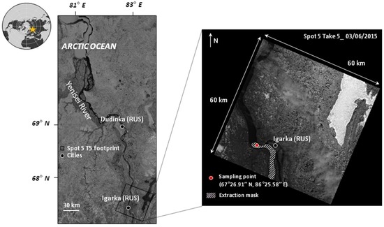
Figure 1.
Map showing the sampling site of DOC and CDOM in the Yenisei River. In 2015, SPOT5 Take5 acquisitions were synchronous with field measurements. Water-leaving reflectances at the sampling location were extracted from an extraction mask.
2.2. Sample Collection and Treatment
Field campaigns were conducted in Igarka, northern Siberia, ~300 km from the basin’s outlet. These campaigns were conducted for two years, from February to September in 2014 and 2015, with the highest temporal resolution during the open-water season (approximately every eight days from May to September), including the freshet period (a few weeks in May and June). Overall, 28 field samples were available in 2014 and 41 in 2015 and were carried out always at the same point in the middle of the river to avoid contamination from the underlying soil and vegetation near the reaches (Figure 1, e.g., 67°26.91′′N ± 00°01′′00–86°25, 58′′E ± 00°01′′00). In 2015, the sampling frequency was increased, and measurements were synchronized with SPOT5 Take5 acquisitions (i.e., on the same day in the morning) every five days from 9 April 2015 to 6 September 2015. From mid-May to the start of July, the field sampling frequency was almost daily.
These samples have been analysed for a number of biogeochemical parameters; here, we focus on the DOC concentrations (mg/L), CDOM (m−1), and TSS concentrations (mg/L).
DOC was analysed on filtered samples (GF/F membrane) after acidification (HCl) to pH 2 using a TOC-V CSH analyser (Shimadzu, Japan). The UV absorption spectra of the filtered samples were measured with a spectrophotometer (Secoman Uvi light XT5) in a 1 cm quartz cell from 190 to 700 nm with a 1 nm resolution. The baseline was determined with ultra-pure water. The CDOM values were retrieved at 440 nm [23]. The values were converted into absorption coefficients (in units of m−1) using Equation (1):
where is the absorbance and the cell path length in meters.
2.3. Extraction of Water-Leaving Reflectance
The study area was selected for the SPOT5 Take5 (ST5) mission. Twenty-five ST5 images were acquired from 9 April 2015 to 6 September 2015 at 10 m resolution and a return interval of five days. Nine images were acquired during the ice-period and were, therefore, left unused (e.g., from 9 April 2015 to 19 May 2015). Six images were cloudy, and four images were contaminated by haze, leading to biased reflectance values. Finally, only six ST5 scenes were retained for this analysis. We also used Landsat 8 (OLI, e.g., L8O) archives (30 m, 16 days) for 2014 and for adding scenes in 2015. Overall, 12 satellite images were selected (Table 1). The largest difference between sampling data and satellite acquisition date was four days.

Table 1.
List of the available SPOT5 Take 5 and Landsat 8 scenes to calibrate an empirical CDOM retrieval algorithm in the Yenisei River during the open-water-season in 2014 and 2015.
The remotely sensed data were atmospherically corrected and converted into surface reflectance values using the MACCS processor for ST5 scenes [46] and the L8SR algorithm for L8O scenes [47]. MACCS determines the aerosol content, the cloud and cloud shadows based on a multitemporal algorithm, while L8SR is a single-date algorithm. As ST5 does not acquire in the blue channel, we only used two spectral bands: green and red wavelengths (e.g., 500–590 nm and 610–680 nm, respectively).
A mask was then manually drawn using GIS software to define the image region where the water reflectance values were to be extracted. This mask had a 15 km north-south extent. Its limits were drawn to 300 m from the riverbanks to avoid contamination by the bank vegetation and the river bed reflectance in shallow water (Figure 1). Finally, we only kept pixels with surface reflectance values below 0.01 to compute the average reflectance in the mask for each band. The goal was to remove pixels affected by sun glint effect or residual ice breaks that were not filtered out by the MACCS and L8SR processors.
2.4. CDOM Algorithm Development
Field-collected CDOM (a440, m−1, N = 69) measurements were used as the dependent variable in a linear regression against the DOC measurements (mg/L) to estimate the relationships of CDOM/DOC in the Yenisei River.
To find the optimal CDOM retrieval algorithm, we considered the relationships already identified in lakes, oceans, or rivers [19,25]. Kutser et al. [19] demonstrated the high performance of a green/red ratio to retrieve CDOM (a420) in 39 lakes in Finland and Southern Sweden (r2 > 0.73). This algorithm was also successfully applied to different datasets [23,28] (r2 > 0.8) with high CDOM values (a440 = 3.4 m−1). Given that SPOT5 and Landsat 8 have these spectral bands, we hypothesized that it could be a relevant model to retrieve the CDOM in the Yenisei River. Griffin et al. [25] also reported an efficient CDOM retrieval algorithm based on the combination of red and green/blue ratios in the Arctic river Kolyma. A similar structure was tested to evaluate the benefits of incorporating an additional band to a band combination on model performances. Finally, models incorporating band multiplication (interaction term) were tested to estimate their capability to retrieve the CDOM.
2.5. Statistical Analyses
All statistical analyses were performed using R 2.3.0.1 software (R Development Core Team 2014, Vienna, Austria) and the “vegan” R package. The relationships between CDOM and the explanatory variables were explored using linear models (LM). The goodness-of-fit was quantified by examining the amount of explained variance (r2), and the root mean square error (RMSE) was also assessed to evaluate the predictive performances of the models.
Overall, seven linear models were tested (Table 2). First, the relationships between CDOM and green or/and red bands were explored Models (1)–(3); second, we focused on models incorporating spectral band combinations. We first evaluated the capacity of the model proposed by Kutser et al. [19] to retrieve CDOM in the Yenisei River, e.g., a green/red ratio Model (4). Model (5) also aimed to analyse the statistical relationships between a green-red combination and the CDOM but with an interaction term, e.g., a green: red interaction. Subsequently, the structure of the model developed by Griffin et al. [25] was investigated. While a first model based on green and green/red ratios was performed Model (6), a second model was built on green and a green: red interaction to retrieve the CDOM in the Yenisei River Model (7). The best statistical model was used to retrieve CDOM and the derived equation from the linear regression between CDOM and DOC was then applied to retrieve DOC concentrations (Figure 2).
Table 2.
Linear regressions tested to retrieve CDOM from green and/or red wavelengths in the Yenisei River.
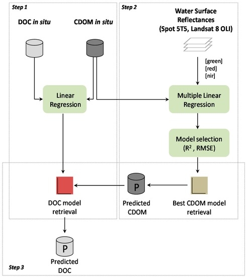
Figure 2.
Methodological flowchart illustrating the general procedure to retrieve DOC concentrations. The Step 1 corresponds to the computation of the DOC model retrieval and the Step 2 indicates the procedure used to predict CDOM values. The Step 3 shows how the DOC model retrieval is finally used to predict DOC concentrations.
2.6. Maps Production
Since no additional exploitable scenes were available in 2014 and 2015 in the study site, DOC maps were produced according to a cross-validation principle (leave-one-out method). In the leave-one-out cross validation, only a single observation is selected for validation (e.g., the date for which the map was derived), and all the remaining observations are used as training data. This process is then repeated such that each observation in the sample is used once as the validation data.
In our case, this procedure was used to predict DOC concentrations at each acquisition date. The single observation selected for validation corresponds to the satellite scene for which the map was derived. Then, we repeated the process until one map was predicted for each date available in our sample set (i.e., 12 times). The maps were produced on the maximum available river channel extent in the ST5 scenes (60 km north-south). The dates were also reorganized according to a theoretical open-water season (i.e., combined 2014 and 2015) to illustrate the potential of high-temporal remote sensing data to map seasonal DOC fluxes.
3. Results
A summary of the laboratory measurements is given in Table 3. The DOC concentrations ranged between 5.03 mg/L and 15.58 mg/L (mean = 8.30, std = 2.93, N = 12) from May to September (i.e., combined 2014 and 2015). The CDOM range was from 1.26 to 10.43 m−1 (mean = 4.93 m−1, std = 2.62−1, N = 12). As expected, the highest DOC and CDOM values were observed in May and June (mean = 10.24 mg/L, std = 2.80, N = 6), e.g., during the peak flow period. The TSS concentrations were found to vary between 2.63 and 19.90 mg/L and were strongly correlated with DOC measurements (r2 = 0.74, p < 0.001, N = 11), indicating that high DOC concentrations occur during high TSS concentrations.
Table 3.
DOC concentrations, CDOM absorption, TSS concentrations, and surface reflectances (SR) at the field sample location.
The CDOM was strongly correlated with the DOC (DOC = 2.13 + 1.24 × (CDOM), r2 = 0.84, p < 0.001). It can, therefore, be used as a proxy to retrieve the DOC concentrations in the Yenisei River (Figure 3). The relationship was computed using all available field samples in 2014 and 2015 (N = 69). This strengthened the statistical relationship CDOM/DOC and improved the DOC retrieval after computation of an empirical model.
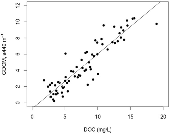
Figure 3.
Relationship between DOC and CDOM in the Yenisei River (DOC = 2.13 + 1.24 × (CDOM), R2 = 0.84, p-value < 0.001). 69 field observations were used from February 2014–September 2014 and April 2015–September 2015.
The model outputs listed in Table 4 show that the best-performing model was based on the green band and a green-red band interaction Model (7). The model exhibited both a high explanatory capability and a high predictive power (r2 = 0.76, RMSE = 1.21). The second best-performing model was built on a similar scheme, but a green-red ratio was included Model (7). Nonetheless, we observed moderate statistical performances from this model (r2 = 0.54, RMSE = 1.68). In addition, the algorithm proposed by [19] did not achieve the expected results (Model (4), r2 = 0.25, RMSE = 2.17), and its counterpart (e.g., with an interaction term, Model (5)) did not provide a satisfying performance (r2 = 0.19, RMSE = 2.25). Finally, models based on green or red bands Models (1) and (2) expressed poor performances (r2 < 0.22, RMSE > 2). The joint incorporation of two spectral bands into a linear model showed better results (Model (3), r2 = 0.44, RMSE = 1.86) but was still not sufficient to retrieve the CDOM in our study site. Indeed, the effects of independent variables in a multiple linear regression model depend on other variables included in the model. Consequently, these results show that the effects of green band on CDOM exclusively depend on the presence of the green: red interaction. Without it, green band cannot explain a significant part of the CDOM variance.
Table 4.
Results of linear regression explaining CDOM at 440 nm (m−1). Slashes are used to express spectral bands ratio, whereas semicolons are used to express spectral bands interaction.
In view of the previous results, Model (7) was selected to retrieve the CDOM in the Yenisei River. A significant negative relationship (−681.477, p < 0.01) between the CDOM and green reflectance values reflects the CDOM absorption of visible light at shorter wavelengths. The green-red interaction had a significant positive effect (16,410.925, p < 0.001) on the CDOM, suggesting that the effect of green band must be interpreted in relation to the red band. The distribution of TSS concentrations was examined under the assumption that they strongly reflect visible light at longer wavelength. The TSS histograms (Figure 4) tended to exhibit two distinct groups of samples with different concentration levels: one with less than 15 mg/L (N = 9) and the other with more than 15 mg/L (N = 3). A negative relationship was observed between the green band and the CDOM when only samples with TSS < 15 mg/L were considered (Figure 5). When the TSS concentrations were low or moderate, the increase of the green reflectance values led to a decrease of the CDOM, as expected. In a situation of high TSS concentrations, increased green reflectance values did not lead to decreased CDOM.
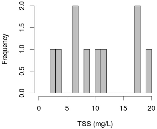
Figure 4.
Frequency distribution of TSS (mg/L) concentrations. Two groups of field sample were distinguished: low or moderate TSS concentrations (TSS < 15 mg/L) and high TSS concentrations (TSS > 15 mg/L).
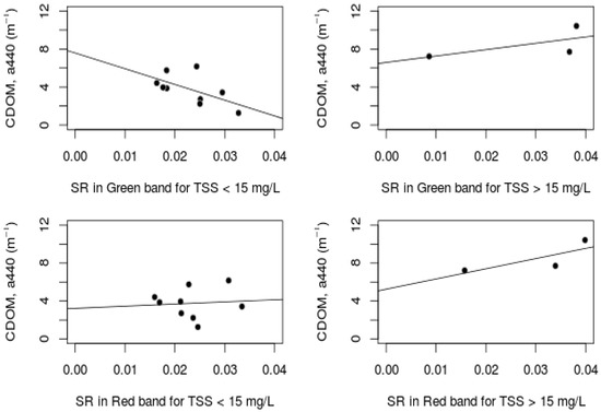
Figure 5.
Statistical relationships between surface reflectance (SR) values in red and green bands and CDOM at 440 nm (m−1) for the two groups of field sample observed from the histogram of frequency (Figure 4). For low or moderate TSS concentrations (TSS < 15 mg/L), the surface reflectance values in green are negatively correlated to CDOM whereas for high concentrations of TSS (TSS > 15 mg/L), the surface reflectance values are positively correlated to CDOM. In the red band, the surface reflectance values are positively correlated to CDOM for the two groups of field sample.
The DOC maps produced from equations derived in Figure 6a,b) showed an expected trend evolution from 22 May 2015 to 8 September, with a linear decrease in colour intensity (Figure 7). The highest values of predicted DOC, e.g., between 14 and 20 mg/L, were mapped during May and June, whereas lower DOC patterns (e.g., <7 mg/L) were predicted as early as the end of July (22 July 2014). At each date, the spatial variability of the predicted DOC in the river channel was moderate (from 0.87 mg/L to 2.22 mg/L). Nonetheless, more intense predicted DOC variations were evident from the upper to the lower part of the meander. Sharp spatial variations in the predicted DOC were also visible near the cloud mask boundaries (13 July and 18 July).
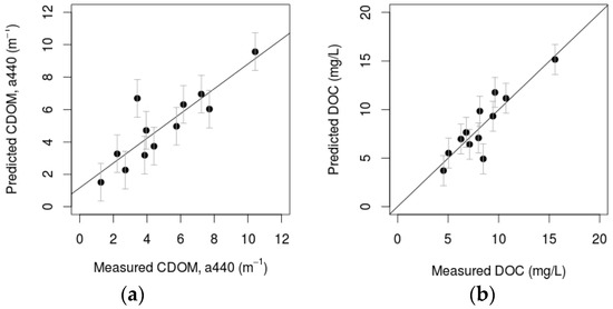
Figure 6.
(a) Relationship between predicted CDOM at 440 nm (m−1) and measured CDOM at 440 nm (m−1) (CDOMpredicted = 1.15 + 0.76 × CDOMmeasured, R2 = 0.76, p-value < 0.001, RMSE = 1.2). (b) Relationship between predicted DOC in mg/L and measured DOC in mg/L (DOCpredicted = 0.02 + 0.99 × DOCmeasured, R2 = 0.79, p-value < 0.001, RMSE = 1.4).
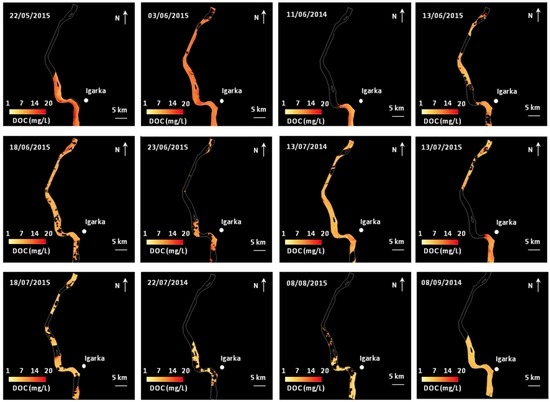
Figure 7.
Mapped DOC during a theoretical open-water season. The best CDOM retrieval algorithm Model (6) was applied on a broader extent (available maximum extent on SPOT5 scenes) to produce estimates of DOC. The maps were produced by a cross-validation method (leave-one-out) and reorganized following a seasonal chronological order, e.g., from 22 May to 8 September (by merging the two years).
4. Discussion
4.1. CDOM and DOC Estimation in Arctic Rivers
Our results demonstrate the capacity of a CDOM algorithm retrieval to estimate the DOC concentrations in the Yenisei River. The CDOM was predicted with an error of 1.2 m−1, and the DOC was predicted with an error of 1.4 mg/L. These findings corroborate the conclusions from previous studies, indicating that CDOM is strongly correlated with DOC in Arctic rivers and constitutes an interesting proxy to supplement and extrapolate DOC measurements in time and space [40,41]. Moreover, the study conducted by [26] recently showed the capability of in situ optical techniques to accurately estimate the amount and timing of terrigenous DOC concentrations in six major Arctic rivers. According to this study, simple absorbance proxies were able to trace dissolved lignin phenol concentrations and seasonal changes of DOM composition in all watersheds studied. Among them, Yenisei expressed the lowest correlation between DOC and CDOM measurements (r2 = 0.66, p < 0.001). Therefore, similar applications to the present study could be potentially tested on other Arctic rivers to improve our understanding of the DOC fluxes from all rivers that flow into the Arctic Ocean.
4.2. Spectral Band Configuration and CDOM Algorithms in Arctic Rivers
The model developed in this study showed better performances than all the other models tested. The models based on one band (e.g., green or red without any combinations; Models (1) and (2)) or two bands were not successful. This demonstrates that linking only one of the two bands with the CDOM is not sufficient to explain its variability. In other words, the CDOM variations on the Yenisei River depended on several drivers that were only captured by using different parts of the visible spectrum via a band combination. However, the incorporation of a single band combination in a model was also insufficient. For example, the algorithm proposed by [19] from a green-red ratio showed poor performances on our data. Using band ratios may be effective if the created range via a band ratio is wider than those of the band alone. Zhu et al. [28] showed that a band ratio is more effective when one band is selected within the range of 400–450 nm and the other band is selected within the range of 630–650 nm. In our case, the green-red ratio allowed us to create a variable with a standard deviation higher than the green or red band (stdgreen/red = 0.20, stdgreen = 0.08, stdred = 0.07) and covered similar parts of the spectrum recommended by [28]; however, the amount of variance explained remained low. Using a single green-band interaction led to similar observations. Although the model indicated significant effects on the CDOM, the green-red interaction only explaining a small fraction of the CDOM variability.
Coupling the green band with a green-red interaction was the most effective band configuration. The green band had a significant negative effect on the CDOM in relation with the CDOM exponential decrease with an increase of wavelengths (e.g., <550 nm). The green-red band interaction also had a significant effect on CDOM, i.e., the effect of surface reflectance in the red on the green/CDOM statistical relationship. We found contrasting effects of the green band, depending on TSS, which was expected to reflect visible light at longer wavelengths (Figure 7). In the situation of low or moderate TSS concentrations, a negative effect of surface reflectance in the green was observed, indicating that other water constituents do not interfere on the expected relationship between the CDOM and the optical remote sensing signal. A positive effect was found in the case of high TSS concentrations, revealing that the noise in the CDOM signal is caused by a significant amount of suspended matter.
These findings reinforce the conclusions of previous studies stating that the algorithm performance can be improved by using an additional longer wavelength because of the significant amounts of particulate matter [28]. These findings highlight the importance of jointly analysing these different signals. Evidence for a potential interactive effect of shorter and longer wavelengths has already been observed in the monitoring of the CDOM in lakes or coastal oceans [19,28]. Brezonick et al. [23] showed differences in the spectra slopes of CDOM in the range of ~570–650 nm for low CDOM levels and high CDOM levels. For low CDOM waters, the spectra declined with increasing wavelength, whereas the opposite trend occurred for high CDOM waters. Hence, because the CDOM levels on the Yenisei River typically belong to the second group, this explains why this method was effective at retrieving the CDOM. Note that the identified TSS level threshold (15 mg/L) is consistent with that mentioned by [25]. Finally, the ARCTIC-Gro project provided point measurements from 2008 to 2014 in six Arctic watersheds (between April and September; [48]). While the Yenisei River contained the lowest TSS concentrations, with an average of 11.3 ± 8.5 mg/L, the other rivers showed much higher TSS values, from 42.0 ± 38.5 mg/L in the Kolyma to 94.6 ± 82.8 mg/L in the McKenzie. Therefore, the development of an effective CDOM algorithm retrieval on all Arctic rivers during the whole open-water season is uncertain.
Indeed, even if the developed empirical model showed high performances, its transferability to different arctic river systems is not straightforward. Applying the model that was successfully calibrated in this study on Kolyma data [25] led to poor results (Table 4, Model (8), r2 = 0.41, RMSE = 3.24 m−1). This result emphasizes that the empirical CDOM retrieval algorithm is not easily transposable to other sites, mainly because of the diverse biogeochemical conditions (DOC and TSS concentrations, chlorophyll, turbidity, etc.), which imply different statistical relationships between the CDOM and the water leaving reflectance [26]. The characteristics of the sensors used can also play a major role. Our model was calibrated from SPOT5 and Landsat 8 data with specific atmospheric corrections. The model can therefore be non-suited to water leaving reflectance from different sensors, as was used in [25] (e.g., Landsat 7). Finally, our model was calibrated to monitor the seasonal DOC concentrations. The model developed using only July and August CDOM/remote sensing relationships did not allow for inter-annual fluxes because, during these months, the CDOM values were moderate (between 1.38 and 6.45 m−1). The model developed was valid for a wide range of CDOM values because it included DOC measurements during the freshet period.
4.3. High Spatio-Temporal Resolution Remote Sensing Data and CDOM in Arctic Rivers
The CDOM algorithm developed in this study is based on high spatio-temporal resolution data. This type of imagery opens two perspectives in the field of DOC monitoring.
First, high spatial resolution (HSR) allowed us to observe the spatial variability of DOC in the river channel at each date. The derived DOC maps showed a low spatial variability in the river channel, with a higher heterogeneity in the meander located in the south of the ST5 footprint. To verify, pixel values were extracted in the area common to all maps (and located in the meander). The standard deviations ranged from ±0.90 mg/L on 9 September 2015 to ±2.40 mg/L on 8 August 2015 and were higher than the predicted error from the developed model on five maps (i.e., >1.4 mg/L). On average, the variability of DOC concentrations after the freshet period was equal to ±1.83 mg/L (e.g., from 13 July 2015) and was higher than those measured during the freshet period (±1.57 mg/L). Its evolution across the open-water season was not correlated to the DOC concentrations or stream flows, indicating that external environmental factors may influence this variability. This heterogeneity could not be observed with a coarser spatial resolution sensor, e.g., MODIS. When the DOC concentrations are high, the observed variability remains relatively low, whereas it could be more problematic when the DOC concentrations are lower (after the freshet period). Moreover, it would be interesting to adapt the sampling protocol by increasing the number of field samples. For example, east-west transects could be reproduced to more accurately quantify the DOC concentration variations into the stream during this period. Concerning sharp variations near the cloud mask boundaries, they were likely caused by cloud adjacency effects occurring at the pixels near the clouds. These effects could be eliminated by a dilatation of the cloud masks. From a methodological perspective, the HSR allowed the optimization of pixel selection to calibrate the statistical models. By drawing a more extensive zone around the sample location, it became possible to retrieve several pixels between clouds. HSR also offered the opportunity to select pixels between remaining ice-breaks. Therefore, we could use a Landsat 8 scene acquired on 22 May, i.e., only a few days after the start of the ice break-period, which is crucial because the DOC concentrations were likely to be very important in this period. Finally, the limitations of HSR imagery could also be listed. Footprints are often limited (60 km × 60 km for ST5 and 190 km × 190 km for LT8) and are not suited to reproducing applications at the largest scale (typically at the watershed scale). The HSR data also had a low temporal frequency over the past decade, which has limited studies on the DOC evolutions over a long time period. Therefore, low-resolution data, such as MODIS, are essential to reconstruct the DOC fluxes over multiple years and thus to link climate variability at a large scale.
Second, high temporal resolution (HTR) enables production of a DOC concentration map time series during a whole open-water season, with six maps during the freshet period. This gives the opportunity to assess the DOC variations during this key period. Next, the HRT increases the probability of acquiring exploitable scenes during this short period. The cloud cover or hazing effects often introduce noise in satellite images acquired in the Arctic regions, masking the region of interest or introducing bias to the surface reflectance values. In this study, we jointly used the ST5 and L8O scenes. This practice is similar to future practices based on Sentinel/Landsat 8 synergies that will allow increased possibilities of obtaining scenes at the same location (all 3–5 days). Hence, our results indicate that this synergy is promising to retrieve CDOM values in Arctic rivers. Nonetheless, the HRT data must be accompanied by high frequency in situ measurements to reduce the time gaps and make the high temporal resolution effective. Finally, atmospheric corrections are assumed to be more accurate regarding the HTR data; such corrections are thought to clearly improve the reliability of the extracted surface water reflectance values. However, this aspect has not been verified, and further comparative studies based on low temporal resolution data should be undertaken to evaluate it in a more quantitative manner.
5. Conclusions
This study demonstrated the capacity of the CDOM algorithm retrieval to monitor DOC fluxes in the Yenisei River during a whole open-water season from high spatio-temporal optical remote sensing data. Therefore, special attention could be given to the freshet period, where six maps of the DOC concentrations were produced. Our findings revealed the interesting use of a shorter/longer wavelength combination to retrieve the CDOM in Arctic rivers. However, perturbations of CDOM signals in the visible spectrum must be taken into account when the TSS concentrations are high.
Using high spatio-temporal optical remote sensing to develop CDOM-based remote sensing algorithms in Arctic rivers can be a very promising method to advance our understanding of Earth’s carbon cycle. However, this method would require an extensive sampling protocol to limit the time gaps between the in situ and spatial measurements, with a high sampling frequency and covering a large period. Future Sentinel 2–3/Landsat 8 synergies should allow for reproducibility of such applications in other hydrological systems. This will open the opportunity to monitor temporal fluctuations of DOC concentrations during the freshet period, as well as the use of the blue band, which could improve CDOM algorithm calibrations. Thus, although low spatial resolution is more problematic from a methodological point of view, coarse remote sensing data, such as MODIS, should be tested in this scope. Low and high spatial resolution imagery could be complementary to improve our understanding of the DOC fluxes from a local to a global spatial scale as well as from a seasonal to decadal scale. Finally, note that the present study site (Igarka, 67°28′19′′N, 86°33′31′′E) was selected for the Sentinel 2 mission. Hence, the surface reflectance products will be delivered for at least two years, and further research on DOC monitoring from space will be conducted.
Acknowledgments
P.A.H was funded by a TOSCA fellowship provided by the French National Spatial Agency (CNES). This work was supported by the french national program EC2CO-Biohefect TOMCAR-Sat (Terrestrial Organic Matter Characterization in Arctic Rivers assessed trough Satellite imagery) and a Marie Curie International Reintegration Grant (TOMCAR-Permafrost #277059) within the 7th European Community Framework Programme. A special thanks to Anatoli Pimov for technical supports on the ground. The Spot-5 Take 5 products were obtained from the Theia Land Data Centre. We are grateful to O. Hagolle for his advices and support during the Take 5 experiment. DOC analysis have been performed at the analytical platform PAPC (EcoLab laboratory) by D. Lambrigot and F. Julien.
Author Contributions
P.A.H developed the methodological framework, performed the analyses, and wrote the article. All authors were involved in the paper review. L.G introduced P.A.H to optical signal of water constituents and S.G to remote Sensing applied to hydrological systems. R.T, N.T, L.G and T.L.D carried out DOC/CDOM field campaigns in the Yenisei River in 2014 and 2015.
Conflicts of Interest
The authors declare no conflict of interest.
References
- Solomon, S.; Qin, D.; Manning, M.; Chen, Z.; Marquis, M.; Averyt, K.B.; Tignor, M.; Miller, H.L. 5th Assessment Report-Climate Change 2013-IPCC; Cambridge University Press: Cambridge, UK, 2013. [Google Scholar]
- Brown, R.; Derksen, C.; Wang, L. A multi-data set analysis of variability and change in Arctic spring snow cover extent, 1967–2008. J. Geophys. Res. Atmos. 2010, 115, D16111. [Google Scholar] [CrossRef]
- Romanovsky, V.E.; Smith, S.L.; Christiansen, H.H. Permafrost thermal state in the polar Northern Hemisphere during the international polar year 2007–2009: A synthesis. Permafr. Periglac. Process. 2010, 21, 106–116. [Google Scholar] [CrossRef]
- Vonk, J.E.; Tank, S.E.; Bowden, W.B.; Laurion, I.; Vincent, W.F.; Alekseychik, P.; Amyot, M.; Billett, M.; Canario, J.; Cory, R.M. Reviews and syntheses: Effects of permafrost thaw on Arctic aquatic ecosystems. Biogeosciences 2015, 12, 7129–7167. [Google Scholar] [CrossRef]
- Lawrence, D.M.; Slater, A.G. A projection of severe near-surface permafrost degradation during the 21st century. Geophys. Res. Lett. 2005, 32, L24401. [Google Scholar] [CrossRef]
- Tarnocai, C.; Canadell, J.G.; Schuur, E.A.G.; Kuhry, P.; Mazhitova, G.; Zimov, S. Soil organic carbon pools in the northern circumpolar permafrost region. Glob. Biogeochem. Cycles 2009, 23, B003327. [Google Scholar] [CrossRef]
- Lemke, P.; Ren, J.; Alley, R.B.; Allison, I.; Carrasco, J.; Flato, G.; Fujii, Y.; Kaser, G.; Mote, P.; Thomas, R.H.; et al. Observations: Changes in snow, ice and frozen ground. In Climate Change 2007: The Physical Science Basis. Contribution of Working Group I to the Fourth Assessment Report of the Intergovernmental Panel on Climate Change; Solomon, S., Qin, D., Manning, M., Chen, Z., Marquis, M., Averyt, K.B., Tignor, M., Miller, H.L., Eds.; Cambridge University Press: Cambridge, UK, 2013. [Google Scholar]
- Zhang, J.; Lindsay, R.; Steele, M.; Schweiger, A. What drove the dramatic retreat of arctic sea ice during summer 2007? Geophys. Res. Lett. 2008, 35, L01505. [Google Scholar] [CrossRef]
- Striegl, R.G.; Aiken, G.R.; Dornblaser, M.M.; Raymond, P.A.; Wickland, K.P. A decrease in discharge-normalized DOC export by the Yukon River during summer through autumn. Geophys. Res. Lett. 2005, 32, L024413. [Google Scholar] [CrossRef]
- Prokushkin, A.S.; Pokrovsky, O.S.; Shirokova, L.S.; Korets, M.A.; Viers, J.; Prokushkin, S.G. Export of dissolved carbon from watersheds of the Central Siberian Plateau. Dock. Earth Sc. 2011, 441, 1568–1571. [Google Scholar] [CrossRef]
- Abbott, B.W.; Jones, J.B.; Schuur, E.A.G.; Chapin, F.S., III; Bowden, W.B.; Bret-Harte, M.S.; Howard, E.; Epstein, M.D.F.; Harms, T.K.; Hollingsworth, T.N.; et al. Biomass offsets little or none of permafrost carbon release from soils, streams, and wildfire: An expert assessment. Environ. Res. Lett. 2016, 11, 034014. [Google Scholar] [CrossRef]
- Kohler, H.; Meon, B.; Gordeev, V.V.; Spitzy, A.; Amon, R.M.W. Dissolved Organic Matter (DOM) in the estuaries of Ob and Yenisei and the adjacent Kara Sea, Russia. In Siberian River Run-off in the Kara Sea: Characterisation, Quantification; Stein, R., Fahl, K., Futterer, D.K., Galimov, E.M., Stepanets, O.V., Eds.; Elsevier Science: Amsterdam, The Netherlands, 2003; pp. 281–308. [Google Scholar]
- Holmes, R.M.; McClelland, J.W.; Peterson, B.J.; Tank, S.E.; Bulygina, E.; Eglinton, T.I.; Gordeev, V.V.; Gurtovaya, T.Y.; Raymond, P.A.; Repeta, D.J. Seasonal and annual fluxes of nutrients and organic matter from large rivers to the Arctic Ocean and surrounding seas. Estuar. Coasts 2012, 35, 369–382. [Google Scholar] [CrossRef]
- Amon, R.M.W.; Rinehart, A.J.; Duan, S.; Louchouarn, P.; Prokushkin, A.; Guggenberger, G.; Bauch, D.; Stedmon, C.; Raymond, P.A.; Holmes, R.M. Dissolved organic matter sources in large Arctic rivers. Geochim. Cosmochim. Acta 2012, 94, 217–237. [Google Scholar] [CrossRef]
- Del Castillo, C.E.; Miller, R.L. On the use of ocean color remote sensing to measure the transport of dissolved organic carbon by the Mississippi River Plume. Remote Sens. Environ. 2008, 12, 836–844. [Google Scholar] [CrossRef]
- Matsuoka, A.; Babin, M.; Doxaran, D.; Hooker, S.B.; Mitchell, B.G.; Bélanger, S.; Bricaud, A. A synthesis of light absorption properties of the Arctic Ocean: Application to semi-analytical estimates of dissolved organic carbon concentrations from space. Biogeosciences 2014, 11, 3131–3147. [Google Scholar] [CrossRef]
- Strömbeck, N.; Pierson, D.C. The effects of variability in the inherent optical properties on estimations of chlorophyll a by remote sensing in Swedish freshwaters. Sci. Total Environ. 2001, 268, 123–137. [Google Scholar] [CrossRef]
- Brezonik, P.; Menken, K.D.; Bauer, M. Landsat-based remote sensing of lake water quality characteristics, including chlorophyll and colored dissolved organic matter (CDOM). Lake Reserv. Manag. 2005, 21, 373–382. [Google Scholar] [CrossRef]
- Kutser, T.; Pierson, D.C.; Kallio, K.Y.; Reinart, A.; Sobek, S. Mapping lake CDOM by satellite remote sensing. Remote Sens. Environ. 2005, 94, 535–540. [Google Scholar] [CrossRef]
- Ylöstalo, P.; Kallio, K.; Seppälä, J. Absorption properties of in-water constituents and their variation among various lake types in the boreal region. Remote Sens. Environ. 2014, 148, 190–205. [Google Scholar] [CrossRef]
- Zhu, W.; Yu, Q.; Tian, Y.Q.; Chen, R.F.; Gardner, G.B. Estimation of chromophoric dissolved organic matter in the Mississippi and Atchafalaya river plume regions using above-surface hyperspectral remote sensing. J. Geophys. Res. 2011, 116, C02011. [Google Scholar] [CrossRef]
- Tian, Y.Q.; Yu, Q.; Zhu, W. Estimating of Chromophoric Dissolved Organic Matter (CDOM) with in-situ and satellite hyperspectral remote sensing technology. In Proceedings of the Geoscience and Remote Sensing Symposium (IGARSS), Munich, Germany, 22–27 July 2012.
- Brezonik, P.L.; Olmanson, L.G.; Finlay, J.C.; Bauer, M.E. Factors affecting the measurement of CDOM by remote sensing of optically complex inland waters. Remote Sens. Environ. 2015, 157, 199–215. [Google Scholar] [CrossRef]
- Fichot, C.G.; Kaiser, K.; Hooker, S.B.; Amon, R.M.; Babin, M.; Bélanger, S.; Walker, S.A.; Benner, R. Pan-Arctic distributions of continental runoff in the Arctic Ocean. Sci. Rep. 2013, 3, 1053. [Google Scholar] [CrossRef] [PubMed]
- Griffin, C.G.; Frey, K.E.; Rogan, J.; Holmes, R.M. Spatial and interannual variability of dissolved organic matter in the Kolyma River, East Siberia, observed using satellite imagery. J. Geophys. Res. 2011, 116. [Google Scholar] [CrossRef]
- Mann, P.J.; Spencer, R.G.M.; Hernes, P.J.; Six, J.; Aiken, G.R.; Tank, S.E.; McClelland, J.W.; Butler, K.D.; Dyda, R.Y.; Holmes, R.M. Pan-Arctic trends in terrestrial dissolved organic matter from optical measurements. Front. Earth Sci. 2016, 4, 25–30. [Google Scholar] [CrossRef]
- Matthews, M.W. A current review of empirical procedures of remote sensing in inland and near-coastal transitional waters. Int. J. Remote Sens. 2011, 32, 6855–6899. [Google Scholar] [CrossRef]
- Zhu, W.; Yu, Q.; Tian, Y.Q.; Becker, B.L.; Zheng, T.; Carrick, H.J. An assessment of remote sensing algorithms for colored dissolved organic matter in complex freshwater environments. Remote Sens. Environ. 2014, 140, 766–778. [Google Scholar] [CrossRef]
- Mannino, A.; Russ, M.E.; Hooker, S.B. Algorithm development and validation for satellite-derived distributions of DOC and CDOM in the US Middle Atlantic Bight. J. Geophys. Res. Oceans 2008, 113, C07051. [Google Scholar] [CrossRef]
- Lee, Z.; Carder, K.; Arnone, R.; He, M. Determination of primary spectral bands for remote sensing of aquatic environments. Sensors 2007, 7, 3428–3441. [Google Scholar] [CrossRef]
- Brando, V.E.; Dekker, A.G. Satellite hyperspectral remote sensing for estimating estuarine and coastal water quality. IEEE Trans. Geosci. Remote Sens. 2003, 41, 1378–1387. [Google Scholar] [CrossRef]
- Wang, P.; Boss, E.S.; Roesler, C. Uncertainties of inherent optical properties obtained from semi-analytical inversions of ocean color. Appl. Opt. 2005, 44, 4074–4085. [Google Scholar] [CrossRef] [PubMed]
- Carder, K.L.; Chen, F.R.; Lee, Z.P.; Hawes, S.K.; Kamykowski, D. Semianalytic moderate-resolution imaging spectrometer algorithms for chlorophyll a and absorption with bio-optical domains based on nitrate-depletion temperatures. J. Geophys. Res. Oceans 1999, 104, 5403–5421. [Google Scholar] [CrossRef]
- D’Sa, E.J.; Miller, R.L. Bio-optical properties in waters influenced by the Mississippi River during low flow conditions. Remote Sens. Environ. 2003, 84, 538–549. [Google Scholar] [CrossRef]
- Fitzmaurice, G. The meaning and interpretation of interaction. Nutrition 2000, 16, 313–314. [Google Scholar] [CrossRef]
- Martinez, J.-M.; Guyot, J.-L.; Filizola, N.; Sondag, F. Increase in suspended sediment discharge of the Amazon River assessed by monitoring network and satellite data. Catena 2009, 79, 257–264. [Google Scholar] [CrossRef]
- Nunes, A.L.; Marçal, A.R.S. Atmospheric correction of high resolution multi-spectral satellite images using a simplified method based on the 6S Code. In Proceedings of the 4th Remote Sensing and Photogrammetry Society Annual Conference-Mapping and Resources Management, Aberdeen, Scotland, 16–18 May 2000.
- Hoge, F.E.; Lyon, P.E. Satellite observation of Chromophoric Dissolved Organic Matter (CDOM) variability in the wake of hurricanes and typhoons. Geophys. Res. Lett. 2002, 29, 141–144. [Google Scholar] [CrossRef]
- Shiklomanov, I.A.; Shiklomanov, A.I.; Lammers, R.B.; Peterson, B.J.; Vorosmarty, C.J. The dynamics of river water inflow to the Arctic Ocean. In The Freshwater Budget of the Arctic Ocean; Springer: Dordrecht, The Netherlands, 2000; pp. 281–296. [Google Scholar]
- Yang, D.; Ye, B.; Kane, D.L. Streamflow changes over Siberian Yenisei River basin. J. Hydrol. 2004, 296, 59–80. [Google Scholar] [CrossRef]
- Serreze, M.C.; Bromwich, D.H.; Clark, M.P.; Etringer, A.J.; Zhang, T.; Lammers, R. Large-scale hydro-climatology of the terrestrial Arctic drainage system. J. Geophys. Res. 2002, 108. [Google Scholar] [CrossRef]
- Stuefer, S.; Daqing, Y.; Shiklomanov, A. Effect of streamflow regulation on mean annual discharge variability of the Yenisei River. IAHS-AISH Publ. 2011, 346, 27–32. [Google Scholar]
- Lobbes, J.M.; Fitznar, H.P.; Kattner, G. Biogeochemical characteristics of dissolved and particulate organic matter in Russian rivers entering the Arctic Ocean. Geochim. Cosmochim. Acta 2000, 64, 2973–2983. [Google Scholar] [CrossRef]
- Dittmar, T.; Kattner, G. The biogeochemistry of the river and shelf ecosystem of the Arctic Ocean: A review. Mar. Chem. 2003, 83, 103–120. [Google Scholar] [CrossRef]
- Amon, R.M.; Meon, B. The biogeochemistry of dissolved organic matter and nutrients in two large Arctic estuaries and potential implications for our understanding of the Arctic Ocean system. Mar. Chem. 2004, 92, 311–330. [Google Scholar] [CrossRef]
- Hagolle, O.; Huc, M.; Villa Pascual, D.; Dedieu, G. A multi-temporal and multi-spectral method to estimate aerosol optical thickness over land, for the atmospheric correction of FormoSat-2, LandSat, VENμS and Sentinel-2 Images. Remote Sens. 2015, 7, 2668–2691. [Google Scholar] [CrossRef]
- USGS. L8SR Product Guide: Provisional Landsat 8 Surface Reflectance Product; (Version 2.0); USGS: Reston, VA, USA, 2015; p. 27.
- McClelland, J.W.; Holmes, R.M.; Peterson, B.J.; Amon, R.; Brabets, T.; Cooper, L.; Gibson, J.; Gordeev, V.V.; Guay, C.; Milburn, D. Development of a Pan-Arctic database for river chemistry. Eos Trans. Am. Geophys. Union 2008, 89, 217–218. [Google Scholar] [CrossRef]
© 2016 by the authors; licensee MDPI, Basel, Switzerland. This article is an open access article distributed under the terms and conditions of the Creative Commons Attribution (CC-BY) license (http://creativecommons.org/licenses/by/4.0/).