Article

Sea-Ice Wintertime Lead Frequencies and Regional Characteristics in the Arctic, 2003–2015

Department of Environmental Meteorology, University of Trier, Trier 54296, Germany
*
Author to whom correspondence should be addressed.
Remote Sens. 2016, 8(1), 4; https://doi.org/10.3390/rs8010004
Submission received: 30 October 2015 / Revised: 4 December 2015 / Accepted: 10 December 2015 / Published: 22 December 2015
(This article belongs to the Special Issue Sea Ice Remote Sensing and Analysis)

Abstract

:
The presence of sea-ice leads represents a key feature of the Arctic sea ice cover. Leads promote the flux of sensible and latent heat from the ocean to the cold winter atmosphere and are thereby crucial for air-sea-ice-ocean interactions. We here apply a binary segmentation procedure to identify leads from MODIS thermal infrared imagery on a daily time scale. The method separates identified leads into two uncertainty categories, with the high uncertainty being attributed to artifacts that arise from warm signatures of unrecognized clouds. Based on the obtained lead detections, we compute quasi-daily pan-Arctic lead maps for the months of January to April, 2003–2015. Our results highlight the marginal ice zone in the Fram Strait and Barents Sea as the primary region for lead activity. The spatial distribution of the average pan-Arctic lead frequencies reveals, moreover, distinct patterns of predominant fracture zones in the Beaufort Sea and along the shelf-breaks, mainly in the Siberian sector of the Arctic Ocean as well as the well-known polynya and fast-ice locations. Additionally, a substantial inter-annual variability of lead occurrences in the Arctic is indicated.

Graphical Abstract

1. Introduction

Almost the entire the Arctic Ocean is covered by sea ice during wintertime and spring. One of the key features of the ice cover is the presence of leads: recurring and elongated areas of open water and thin ice. The World Meteorological Organization (WMO) defines a lead as a more than 50 m wide crack in the ice from several kilometers to hundreds of kilometers in length. Leads promote a very strong exchange of heat and moisture between the relatively warm ocean and the cold winter atmosphere (e.g., [1,2]). Consequently, a considerable fraction of new ice is produced in leads, thereby contributing to the seasonal sea-ice mass balance of the whole Arctic. Leads have moreover been recognized as a source of global methane emissions, which makes them a potential driver for greenhouse gases [3]. The recurrence of leads and their spatial distribution are valuable diagnostic parameters for the sea-ice drift [4] and changes in the sea-ice stability [5] and represent an essential habitat for marine mammals and birds [6]. Hence, especially in light of the observed trends in Arctic sea-ice extent ([7,8,9]), and with respect to the projected future changes in the Arctic climate system, the structure and dynamics of leads represent essential information for global change monitoring, e.g., [10]. The spatial resolution of sea-ice models is generally too coarse to simulate leads explicitly. Therefore, the sub-grid lead fraction in global and regional sea-ice/ocean models is mainly parameterized [11]. As leads have a strong impact on the atmospheric boundary layer (e.g., [12,13]) and via atmospheric forcing and sea ice production also on ocean processes [14], verification data sets for lead parametrization are needed.
The identification of sea-ice leads from remote sensing data is addressed in many studies using different types of data and focusing on different Arctic regions. Fily and Rothrock [15] apply image cross correlation techniques with radar imagery to identify lead opening and closing areas. Key et al. [16] detect leads by means of thermal infrared and visible satellite imagery. They focus on the retrieval of lead width for some image frames. In a similar manner, binary lead maps for specific Arctic regions are produced from Advanced Very High Resolution Radiometer AVHRR data by Lindsay and Rothrock [17] using the concept of potential open water per pixel and a fixed threshold that is evaluated by comparison with visible data. Drüe and Heinemann [18,19] apply a similar technique using Moderate Resolution Imaging Spectroradiometer (MODIS) data with adaptive thresholds in a moving 51 × 51 pixel kernel. A detection of leads in the western Arctic from optical satellite data for the winters from 1979 to 1985 is presented by Miles and Barry [20]. More recent studies address the potential of shape-constrained segmentation of ice floes [21] and the detection of leads from airborne visible imagery [22] for single case studies. Mahoney et al. [23] present a large-scale mapping and characterization of springtime leads in the Beaufort and Chukchi Seas based on optical and thermal infrared satellite imagery. The potential of radar altimetry for a detection of leads is investigated by Wernecke and Kaleschke [24] and Zakharova et al. [25]. The first long-term pan-Arctic lead data set is provided by Röhrs et al. [26]. They use passive microwave data to derive daily lead concentration maps for the entire Arctic. Bröhan and Kaleschke [27] derive a nine-year climatology of lead orientations based on this data set. A new technical approach to derive pan-Arctic lead maps from thermal-infrared imagery is suggested by Willmes and Heinemann [28]. They test different automatic segmentation techniques and introduce a filter that removes artifacts in the lead classification that arise from warm signatures of unidentified clouds. So far, no product exists that yields pan-Arctic lead maps at a resolution higher than 5 km on a daily basis. However, such a data set would be highly valuable for the verification, assessment and parametrization of global climate models, ice drift patterns, atmosphere-ice-ocean processes and a comparison with sea-ice concentration data, e.g., Spreen et al. [29].
In the present study, daily wintertime (January to April) pan-Arctic lead maps are derived from MODIS thermal infrared imagery for the years of 2003 to 2015 using the method introduced by Willmes and Heinemann [28]. First, we show exemplary results of the retrieval and introduce what we refer to as quasi-daily pan-Arctic lead maps. Subsequently, we describe the computation of monthly and annual wintertime lead frequency maps. Based on these results, we investigate the general spatial distribution as well as the seasonal and inter-annual variability of sea-ice lead frequencies in the Arctic. Finally, we discuss potential causes for the most prominent spatial patterns of the identified leads.

2. Data and Methods

2.1. Satellite Data

We use thermal-infrared data from the MODIS sensor to identify sea-ice leads by means of their warm signature in comparison to the colder thick and snow-covered sea ice during wintertime. MODIS is an instrument on board the two polar orbiting satellites Terra and Aqua, which are part of the U.S. National Aeronautics and Space Administration (NASA’s) Earth Observing System (EOS). Terra MODIS and Aqua MODIS view the entire Earth’s surface every 1–2 days, acquiring data in 36 discrete spectral bands from the optical to the thermal infrared wavelength region. The swath width of MODIS is 2330 km. Continuous measurements are combined to so-called “tiles” after every 5 min of acquisition, resulting in an array with 2030 (“along-swath”) × 1354 (“across-swath”) grid points. The MODIS MOD29/MYD29 data set is a gridded product [30,31] that provides ice surface temperatures with an accuracy of 1–3 K under clear-sky conditions with a geometric resolution of 1 km 2 at nadir decreasing to approximately 4 km 2 at the swath edges. MOD29/MYD29 ice surface temperatures are obtained from the U.S. National Snow and Ice Data Center (NSIDC) (n5eil01u.ecs.nsidc.org/SAN/). We use all available swaths from the MOD29/MYD29 data set that cover the region north of 65 N. This pre-selection was carried out using the meta data available for each MODIS swath. The MODIS cloud mask (MOD/MYD35) is integrated in the product; however, the cloud-mask algorithm has difficulties in identifying sea smoke and thin low clouds [32,33,34], especially during the polar night, which eventually results in high ice surface temperatures (which we here refer to as cloud artifacts) that are not attributed to real surface features. Although improvements were achieved [35], confident cloud cover detection in polar nighttime over snow and ice surfaces remains a problem. This shortcoming is mitigated in our analysis by applying a fuzzy cloud artifact filter [28]. For a qualitative comparison of our daily lead maps with optical data and to demonstrate the filter performance, we here use the MODIS Surface-Reflectance Product (MOD/MYD09; [36]). MODIS Surface Reflectance is a seven-band product computed from the MODIS Level 1B land bands 1 to 7. The product is an estimate of the surface spectral reflectance at ground level assuming no atmospheric scattering or absorption. We here use surface reflectance from channel 2 and first normalize reflectance data for each swath between 0 and 1. Subsequently, the daily composite is prepared by projecting all available normalized reflectance swath data to the pan-Arctic grid and average reflectance over the stack where multiple data points are available. The date of 4 April 2009 was chosen for a qualitative comparison because the overall cloud coverage was low in the regions of interest during this day. By using reflectance data, leads are detected as dark signatures in comparison to the surrounding sea ice. For an operational lead retrieval during wintertime, reflectance data are less useful because of the lack of sunlight.

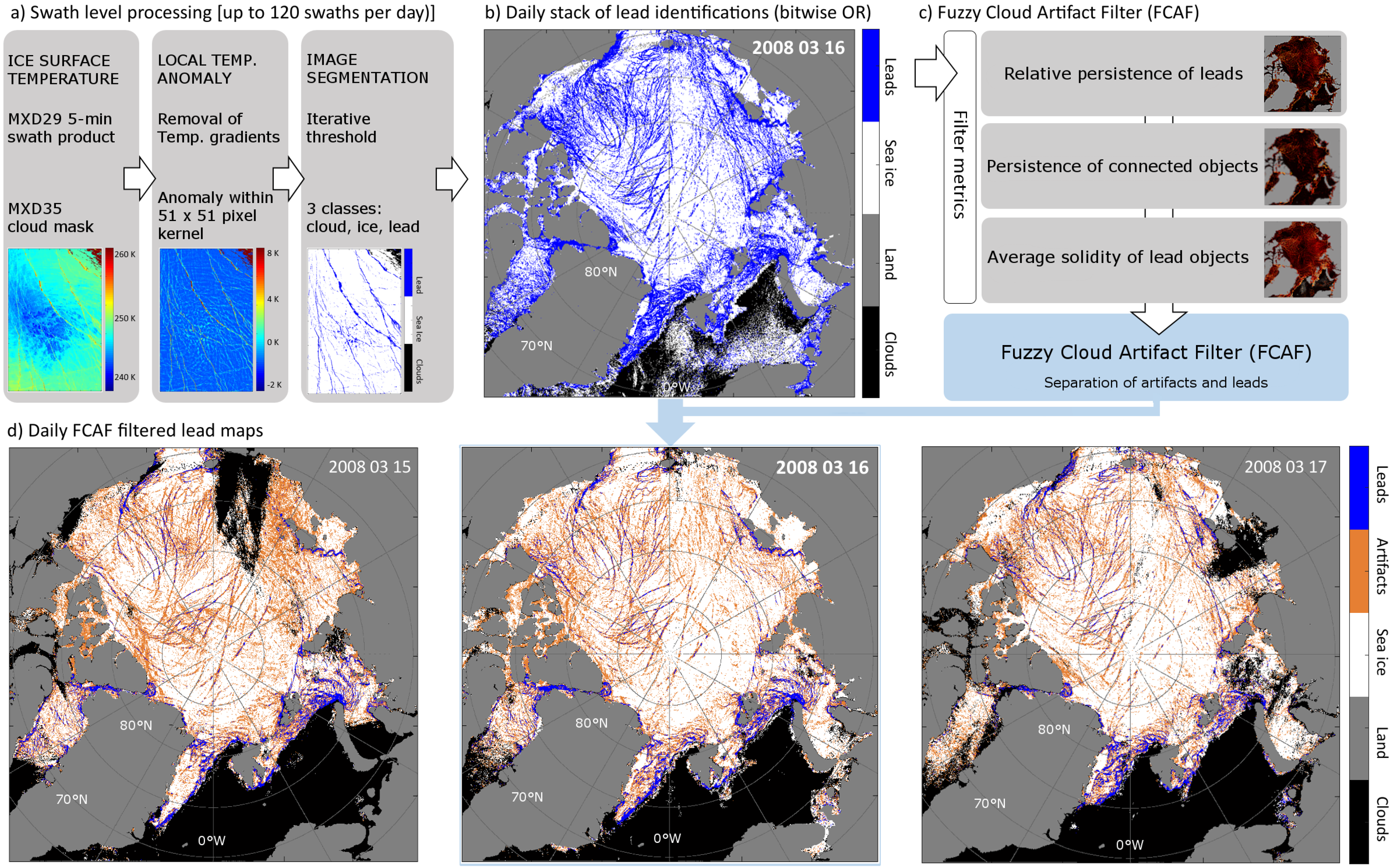
2.2. Sea-Ice Lead Detection

Our lead retrieval method is based on the detection of significant positive surface temperature anomalies. Assuming that the presence of a lead exhibits a warm signal with respect to its surrounding region, we use the MODIS surface temperature product (e.g., Figure 1a, left box) and in a first step remove swath-level temperature gradients by deriving the local temperature anomalies based on the surface temperature distribution in a 51 × 51 pixel kernel (Figure 1a, middle box). Subsequently, the temperature anomaly map is segmented into sea-ice and lead categories applying an iterative threshold procedure that separates the “warm tail” of the obtained temperature anomalies from the given range of values. Since we apply a swath-wise segmentation without an across-swath normalization of surface-temperature anomalies by fixed tie points (e.g., freezing temperature of sea water), the segmentation shows only a small sensitivity to weather-induced changes in the background (thick-ice) surface temperature. Our study is limited to the months of January to April because our segmentation relies on a pronounced thermal contrast between leads (thin ice or open water) and the surrounding thick ice, which requires excluding the potential influence of warm surface signatures in the freeze-up and early melt seasons. As a result, we obtain a three-category map with sea ice, lead and cloud pixels from each surface temperature tile image while the cloud class is taken over from the cloud mask that is integrated in the MOD/MYD29 product (Figure 1a, right box). The method and applied threshold techniques are described in detail in Willmes and Heinemann [28].

2.3. Aggregation of Daily Maps

The obtained three-class images are projected to a polar stereographic pan-Arctic grid with a spatial resolution of 1.5 km. A nearest-neighbor interpolation is performed to account for the categorical character of the segmented images. A daily aggregate is obtained applying a logical disjunction (bitwise OR) operation on the lead class such that every identified lead in a segmented swath image is marked as a potential lead pixel in the pan-Arctic binary daily aggregate (Figure 1b). Additionally, a second aggregate is produced that accumulates the lead identifications for each pixel and thereby provides a persistence indicator for the subsequent filtering procedure. Pixels that are not subject to a sea ice or lead detection are assigned to the cloud category. Due to the convergence of satellite ground tracks in high latitudes and the associated increased probability of a clear-sky view within 24 h, the cloud category can often be replaced by either sea-ice or lead detections (see also Section 2.3).
Figure 1. Retrieval of quasi-daily lead maps. (a) MODIS tile processing for 16 March 2008. After segmentation, the tile is projected to a common polar stereographic grid; (b) the resulting stack of daily potential lead identifications, resulting from a bitwise OR operation where leads from all tiles are combined; (c) Retrieval of temporal (lead pixel persistence, object persistence) and spatial (average solidity per lead pixel) metrics that are used in the Fuzzy Cloud Artifact Filter (FCAF) filter system [28] ); (d) FCAF filtered daily lead aggregate with categories cloud, land mask, sea ice, artifacts and true leads, three consecutive days 15 to 17 March 2008.
Remotesensing 08 00004 g001

2.4. Cloud Artifact Filtering

Unidentified clouds with a warm signature eventually cause erroneous lead detections in the daily binary aggregate which are often characterized by a low temporal persistence (cloud moves faster than leads drift) and low eccentricity. We therefore apply what we refer to as a Fuzzy Cloud Artifact Filter (FCAF) making use of the daily binary lead aggregate in terms of (1) the daily persistence of lead identifications per pixel; (2) the connectivity of lead objects and their persistence and (3) characteristic spatial features, i.e., solidity, which represents a measure of the eccentricity of lead objects from the daily binary aggregate. The parameters (1) to (3) are used as input to the FCAF (Figure 1c) to distinguish between true leads and artifacts that arise from warm surface features caused by unidentified clouds. The separation is based on the definition of rules with associated weights that assign characteristic values of the parameters (1) to (3) and their combination to one of either class, lead or artifact. The rule weights were tuned based on a set of manually classified images. The entire filter process is thoroughly described in Willmes and Heinemann [28]. They optimize the FCAF performance such that the lead class error is reduced to 5% while the error in the artifact class remains at roughly 50%. This means that leads are identified in the lead class with high confidence (95%), which comes at the cost of a conservative artifact class that still contains 50% of true leads that cannot be properly separated from artifacts with the current filter design. The resulting map thus divides the lead class from the daily binary aggregate (Figure 1b, blue regions) into artifacts and true leads (Figure 1d, orange and blue, respectively). A sequence of three FCAF filtered daily lead maps for consecutive days from 15 to 17 March 2008 is shown in Figure 1d. Each map contains one of five categories: clouds, land mask, sea ice, artifacts and leads. These maps are provided daily for the months of January to April for the years from 2003 to 2015 and represent what we consider as quasi-daily pan-Arctic lead maps, while leads are provided in two uncertainty classes (5% and 50% for leads and artifacts, respectively). These maps are available at the PANGAEA Data Publisher for Earth and Environmental Science data (http://dx.doi.org/10.1594/PANGAEA.854411).

3. Results

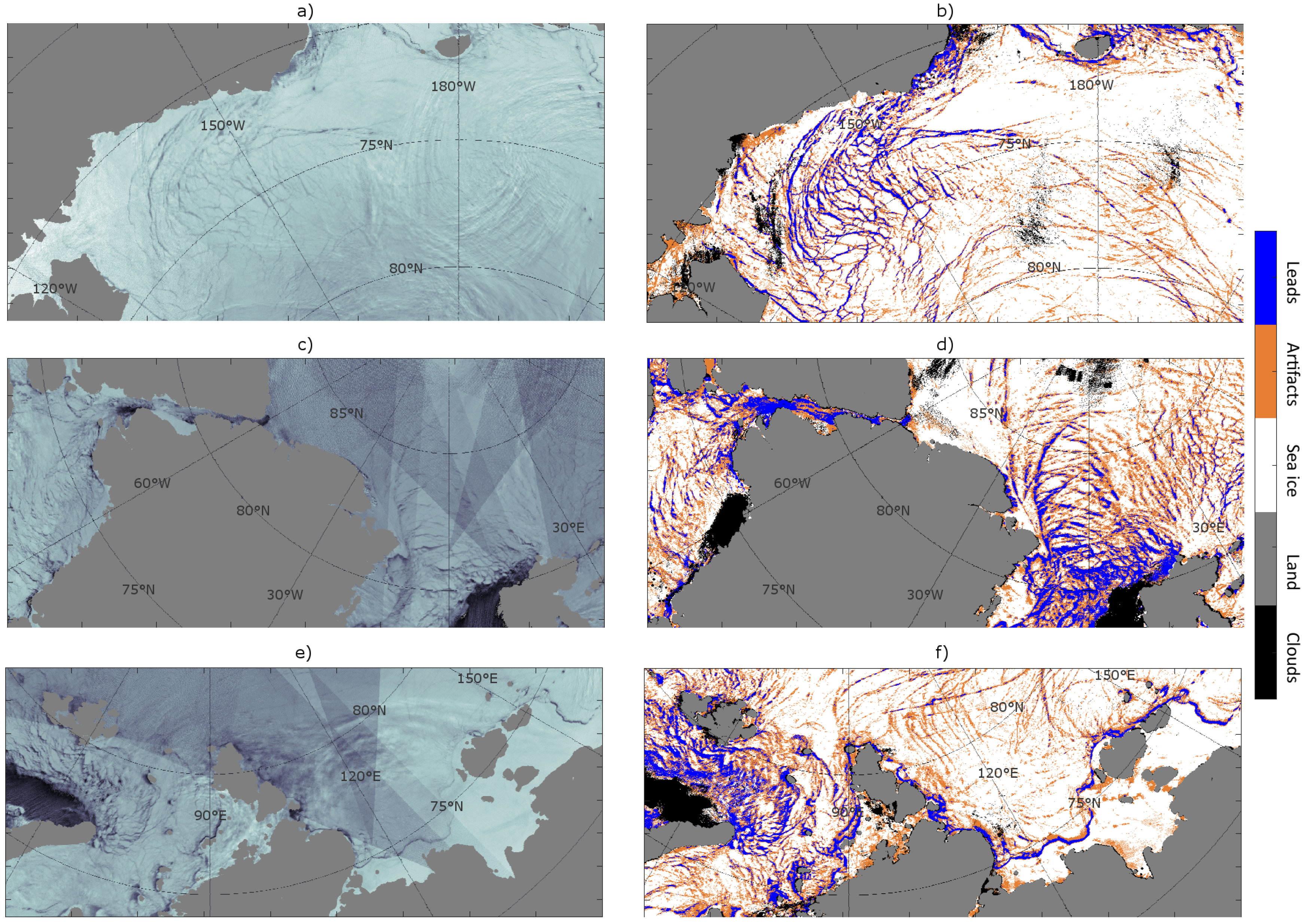
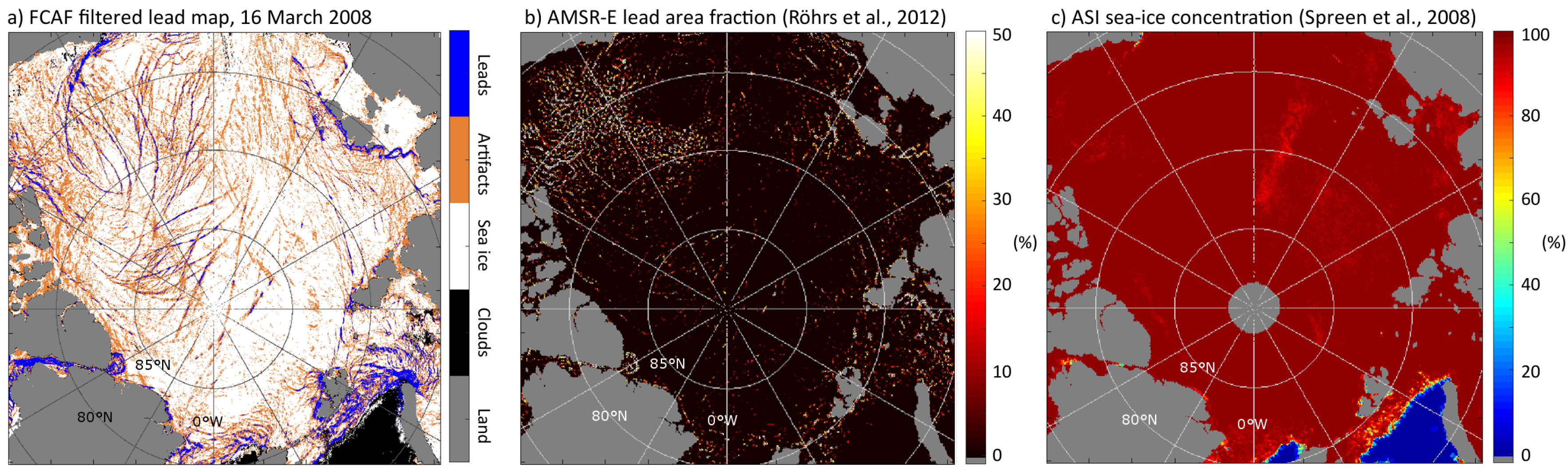
3.1. Segmentation and Filter Performance

Some examples of the segmentation and filter results are shown in Figure 2, comprising daily aggregated MOD/MYD09 normalized reflectance as a qualitative lead occurrence reference in the left column and FCAF filtered daily lead maps for the same subset and day in the right column. The comparison is meant to provide only a qualitative measure since changes in the reflective signature of leads do not necessarily need to be congruent with changes in their thermal signature, i.e., a lead covered with thin ice and snow can still exhibit a substantial warm temperature anomaly while its reflectance may already approach a characteristic value for thick sea ice. Nevertheless, all three subsets indicate that the FCAF captures the most significant leads (blue), i.e., dark regions in left column, very well and achieves a reasonable separation from warm surface features that are not associated with real leads (orange). While the lead class confidently represents what can be recognized as leads also in the reflectance data, the artifact class comprises both, erroneous lead and also some apparently true leads, which aligns with the 50% uncertainty of the artifact class mentioned before.
Figure 2. Comparison of swath-normalized and daily averaged reflectance (left column, MODIS channel 2) and FCAF output data (right column), 4 April 2009, for (a,b) the Beaufort and Chukchi Seas; (c,d) the Greenland Sea, northern Baffin Bay and northern Fram Strait; (e,f) in the Kara and Laptev Seas.
Remotesensing 08 00004 g002

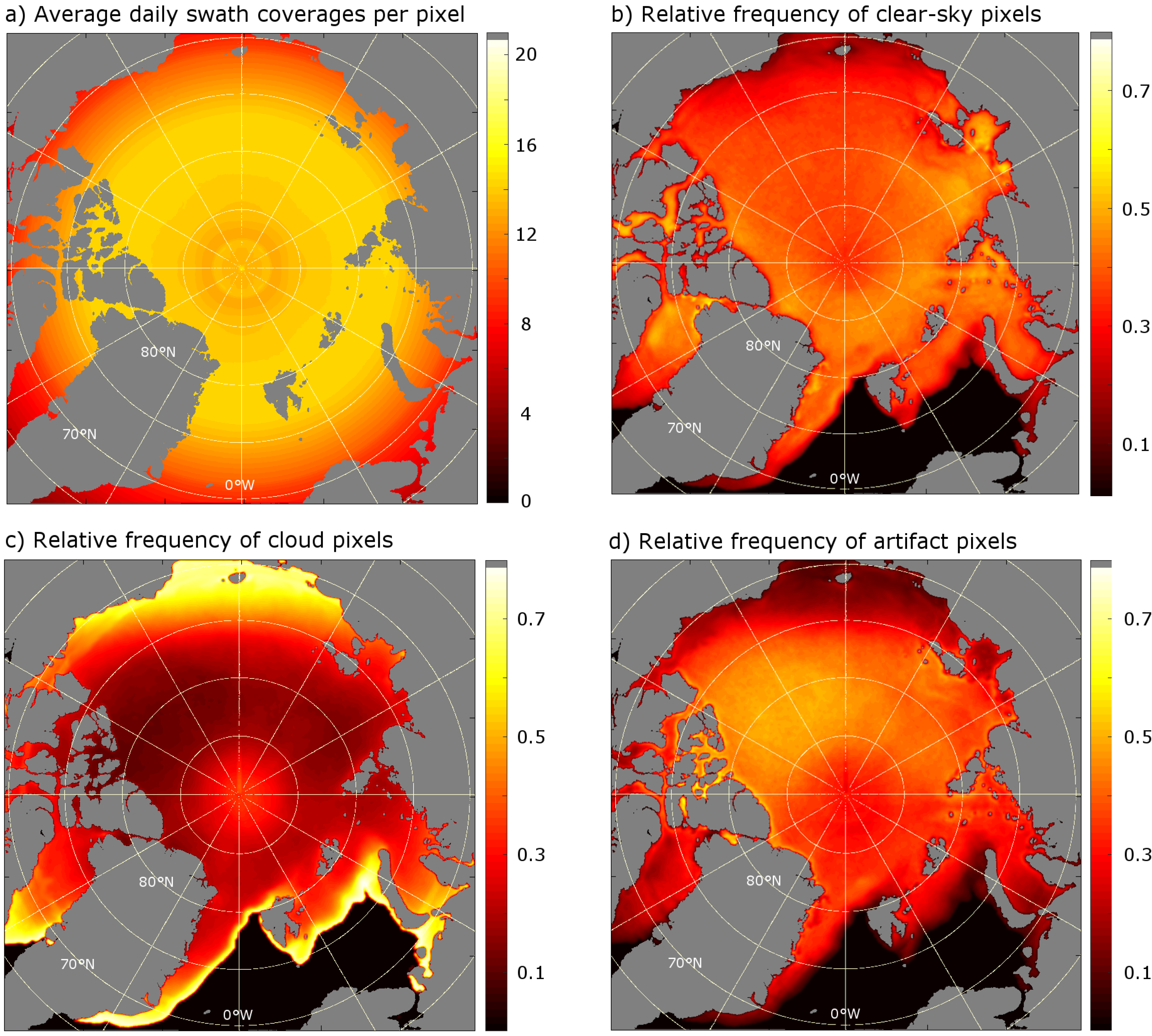
3.2. Data Availability

Figure 3a shows that, due to the convergence of satellite tracks towards higher latitudes, multiple overpasses are available during the course of one day in the region of interest. The average number of ice surface temperature data per pixel and day reaches up to 20 values with a mean of approximately 16 values in the main region of interest. The lowest coverage with only six surface temperature data per pixel and day within the sea-ice covered region is found in the Chukchi Sea, which reaches down to latitudes of 65 N. The probability of occurrence of clouds increased towards lower latitudes which is why we limit our study region here to 65 N. A total of 1560 FCAF filtered daily lead maps (discarding leap year days) is available for the months of January to April in the years from 2003 to 2015. The spatial distribution of the relative frequency of the different categories is highlighted in Figure 3c–e for clear-sky (lead or sea ice), cloud and artifact detections, respectively. One can see that the region of interest provides on average a clear-sky frequency of 30%–60% in the daily aggregates. The lowest availability of clear-sky data is again found in the Chukchi Sea, where the daily number of swath data is also lowest. This results in a lower probability for a given cloud pixel to be replaced by a clear-sky view and, hence, the highest cloud pixel frequency in the same region (Figure 3c). It has to be noted that the cloud pixel frequency provided here does not represent the spatial distribution of cloud occurrences in the Arctic, but rather a measure for the probability that a cloud pixel could be replaced by a clear-sky view using the entire stack of swath data for one day. The cloud pixel frequency is hence, at least in parts, a function of the data provided in Figure 3a. A comparison between clear-sky and artifact frequencies reveals that artifacts are slightly more frequently found in the Northern Beaufort and Laptev Seas, while clear-sky pixels are more abundant in the Atlantic and southern Siberian sectors of the Arctic.

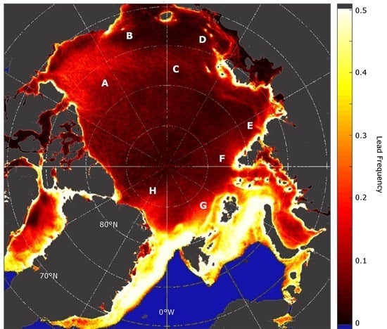
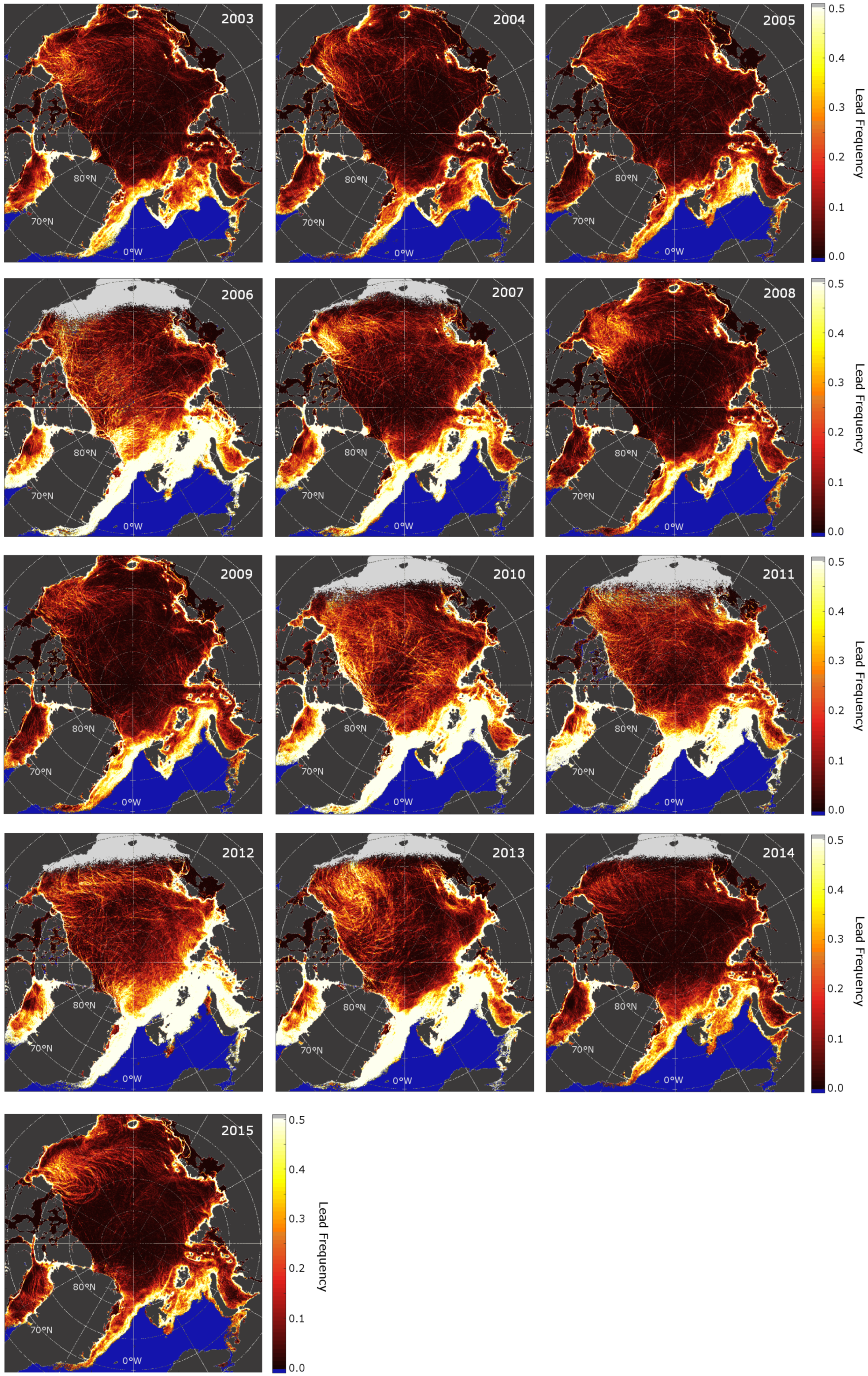
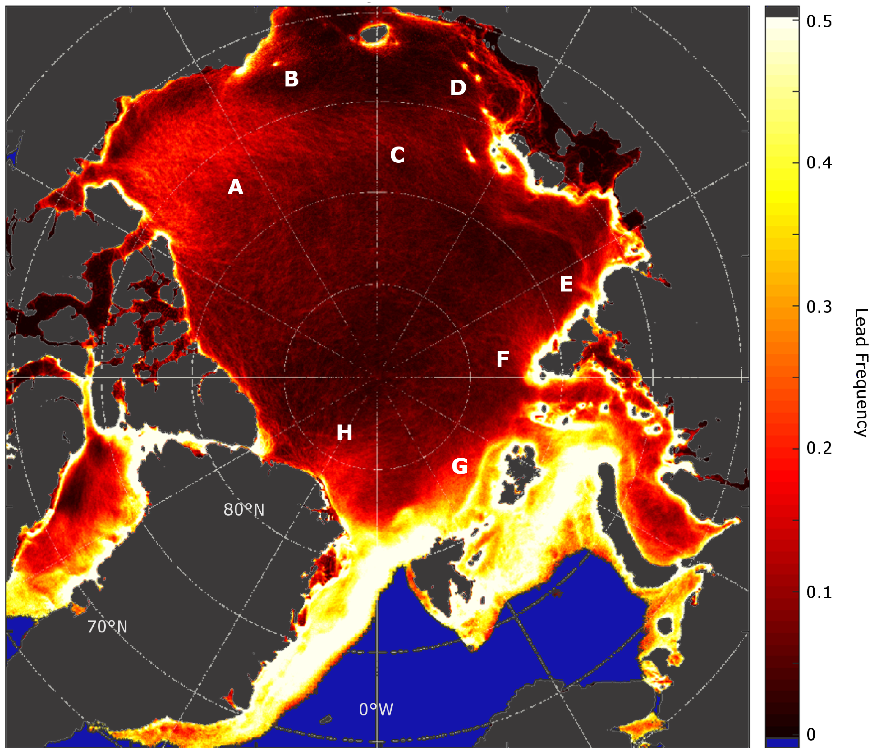
3.3. Sea-Ice Lead Frequencies and Distribution

The quasi-daily lead maps (e.g., Figure 1d) can be used to monitor daily changes in the pan-Arctic distribution of leads. We here derive monthly and annual aggregates for the months of January to April to give insight into the seasonal and inter-annual dynamics of lead occurrences in the Arctic. The aggregation is performed by building the ratio of lead counts per pixel and month (or year) over the total number of clear-sky counts in the same period. As shown in Figure 3b, the clear-sky period that can be used to calculate this ratio covers on average 30% to 60% of the entire period of interest. In doing so, we assume the derived lead frequency to be representative also for the period when clouds or artifacts were present. The artifact class can be included in the lead frequency retrieval when its 50% uncertainty is accounted for. This alternative calculation extends the period for which the representative ratio is derived (clear-sky + artifact occurrences), however, at the cost of an increased uncertainty from the artifact class. In the end, the monthly and annual aggregate maps do not change notably when the alternative calculation is performed, which is why the maps shown here were derived from clear-sky pixels only (no artifacts considered). In cases when the clear-sky frequency is very low, it is questionable whether the assumption that the derived lead frequency also holds for days with clouds or artifacts still holds. Therefore, we define a minimum clear-sky frequency of 0.15 for the aggregation period (month or year) that must be met for a lead frequency to be calculated. The spatial distribution of the annual wintertime (January to April) lead frequencies for the years of 2003 to 2015 is shown in Figure 4. Regions where the 0.15 clear-sky frequency criterion is not met are masked by gray color. These regions obviously occur exclusively in the area of the Chukchi Sea and slightly northwards (compare Figure 3) in the years of 2006, 2007 and 2010 to 2014. As for the remaining years and regions, the given wintertime lead frequencies reveal a substantial spatial and temporal variability. In all of the presented years, the marginal ice zone (MIZ) can be clearly identified as a region with the highest lead frequencies (>0.5). Nevertheless, the strength of this signal shows also a substantial inter-annual variability, which is indicative of the variability in the divergence characteristics of the MIZ. The years of 2006, 2007 and 2010 to 2013 show a pronounced lead signal in the MIZ, whereas this is obviously weaker in the remaining years. Another obvious feature in the lead aggregates is the representation of polynyas and fast ice [37]. Especially the extended fast-ice regions in the Siberian Arctic, but also the Norske Øer Ice Barrier at the Northeast coast of Greenland [38] can be easily identified by their very low lead frequencies. In contrast, the characteristic Siberian flaw polynyas in the Kara, Laptev and East Siberian Seas as well as the North Water polynya between Greenland and Ellesmere Island are pinpointed by high lead frequency values. However, also in the other sea-ice areas, a substantial variability of lead occurrences can be found. Noteworthy is mainly a recurring significant lead pattern in the Beaufort Sea, potentially indicative of the shear that is induced by the Beaufort Gyre. Inter-annual changes in this lead pattern are clearly present. Monthly (January to April) maps of average lead frequencies for the years of 2003 to 2015 are provided as a supplement to this paper.
Figure 3. (a) average number of swath coverages per day; (b) relative frequency of clear-sky pixels (lead or sea ice detections); (c) relative frequency of cloud pixels remaining in the daily aggregate and (d) relative frequency of artifact detections; (b) to (d) relative to the total number of days, January to April, 2003–2015 (n = 1560 days). Values in (b–d) add up to 1.
Remotesensing 08 00004 g003
Figure 4. Annual lead frequencies, January to April, 2003–2015, frequency values are cut off at 0.5 to better highlight the variability at lower values. Grey areas denote regions with a clear-sky frequency less then 15%. (In supplement: Monthly lead frequencies, 2003–2015).
Remotesensing 08 00004 g004

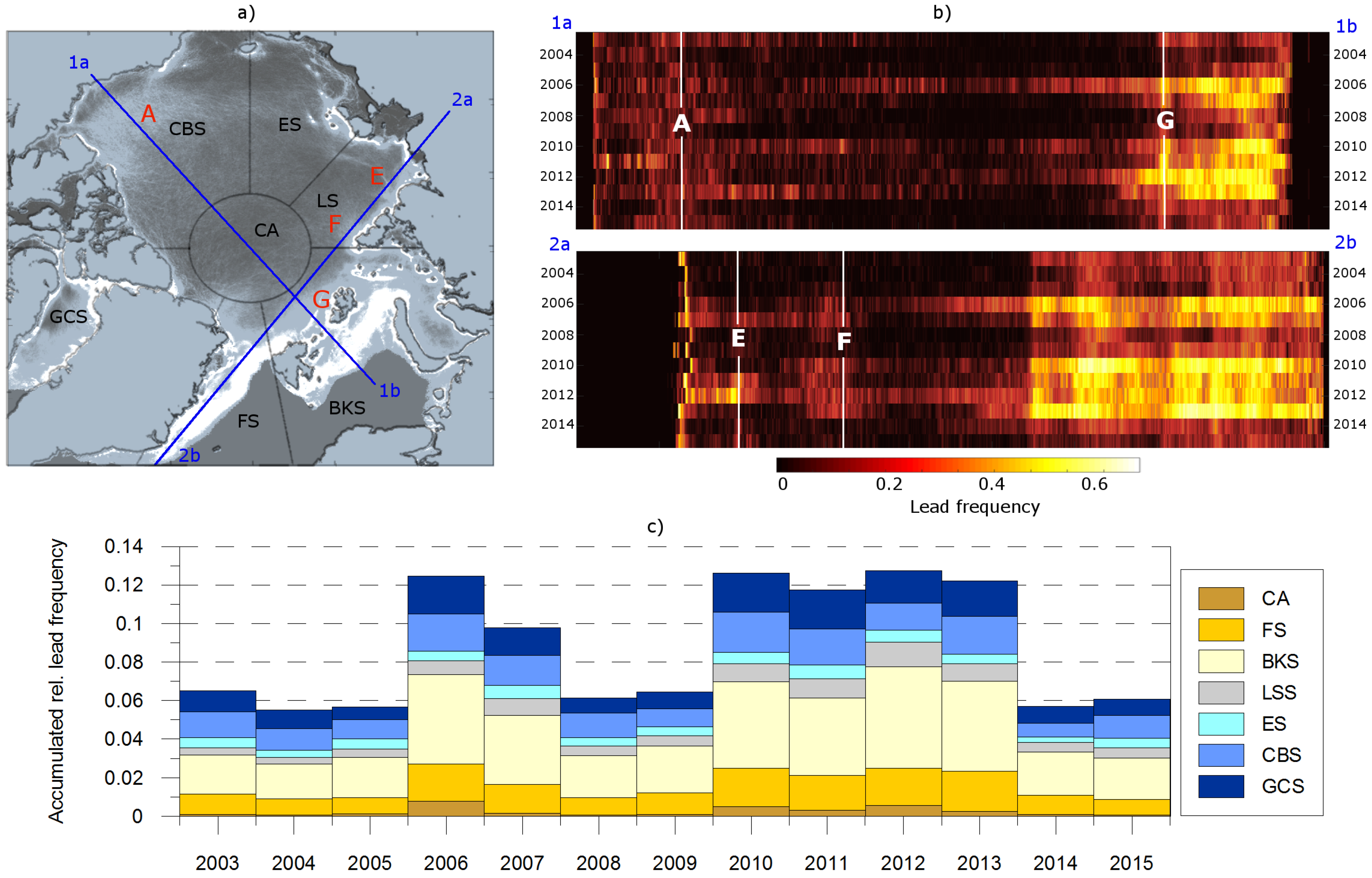
3.4. Spatial and Temporal Lead Dynamics

If the lead aggregation is performed for the entire period of investigation from 2003 to 2015, we obtain valuable insight in the general pattern of lead occurrences in the entire Arctic (Figure 5). As in the annual maps, the MIZ as well as the characteristic polynya regions are well represented by high lead frequencies, whereas the opposite is again found for fast-ice regions. The position of the fast-ice edge in the East Siberian Sea is characterized by higher variability than e.g., in the Laptev Sea. Again, the Beaufort Sea is revealed as an area of major lead activity within the pack ice zone (A). Major shear zones and the associated higher frequency of leads are generally found in the proximity of islands and continental coasts. In addition, smaller characteristic features are highlighted in the presented map, e.g., Hanna Shoal, in the Northern Chukchi Sea (B, [23,37]), is clearly revealed as a significant hot spot of high lead frequencies in the presented map. A band of slightly enhanced lead activity that reaches from the central Beaufort Sea to the new Siberian Islands is visible (C) and in the East Siberian Sea, some less known features exhibiting high lead frequencies are indicated north of the Kolyma Gulf (D). They seem to stem from the presence of several small shoals in this region. An enhanced lead activity is also found in the outflow of the Vilkitzky canyon in the western Laptev Sea (E) and in the shear zone east of Severnaya Zemlya (F). In the northwest of Franz-Josef Land, an elongated region of high lead frequencies (G) is also revealed. As the features shown in E and G are probably not connected shear zones, we speculate that they might be promoted by bathymetric effects (see discussion). The region North of Greenland, at the western edge of the Transpolar Drift stream (H) is also characterized by a higher frequency of leads as compared to the surrounding region.
Figure 5. Average pan-Arctic lead frequencies from daily FCAF filtered lead maps, January to April, 2003–2015. A cut-off value of 0.5 is applied to highlight patterns in the value range 0 to 0.5. Highlighted regions: A = Beaufort Sea, B = Hanna Shoal, C = Band between the Beaufort Sea and New Siberian Islands, D = two unknown lead hot spots in the East Siberian Sea, E = Vilkitsky canyon outflow region, F = fracture zone east of Severnaya Semlya, G = Elongated region with high lead frequency northwest of Franz Josef Land and H = enhanced lead activity north of Greenland.)
Remotesensing 08 00004 g005
We here define two transects crossing the Arctic Ocean to provide insight into the spatial-temporal variability of leads dynamics from 2003 to 2015 (Figure 6a). Transect 1 goes from the coast of the Beaufort Sea, crossing the North Pole, to the Barents Sea. Transect 2 starts in Siberia, and from there crosses the western Laptev Sea, the Transpolar Drift and Fram Strait through the entire MIZ. Hovmoeller plots for the two transects and the years from 2003 to 2015 are shown in Figure 6b with interesting regions (compare Figure 5) highlighted by A (Beaufort Sea), G (a characteristic lead hot spot northwest of Franz-Josef Land), E (the Vilkitzky canyon outflow) and F (the shear zone northeast of Severnaya Zemlya. A substantial inter-annual variability (change along columns) is apparent in all regions, with the coastal polynyas representing the most stable feature. In addition, the Beaufort Sea (A) is characterized by pronounced lead activities in all the years observed with the meridional extension of the main lead activity showing an intense variability. The significant lead region northwest of Franz-Josef Land (G) exhibits a clear signal in almost all of the presented years, which is even similar to the lead frequencies that are found in MIZ (right of number 2 in Figure 6b). The same holds for the region where the Vilkitsky Strait Current [39] enters the Laptev Sea (E) and the shear zone east of Severnaya Zemlya (F).
From the daily FCAF filtered lead maps, we derive the inter-annual variability of pan-Arctic lead dynamics by calculating the accumulated per-region lead frequency (Figure 6c). One can see that especially the years of 2006, 2007 and 2010 to 2013 exhibit a positive anomaly in the pan-Arctic lead activity, which is caused by high lead frequencies in almost all of the presented sub-regions. As far as regional differences are concerned, the largest number of leads occurs in the Fram Strait (FS) and Barents/Kara Sea (BKS) regions, where the marginal ice zone is located, while the central Arctic (CA) is characterized by low lead frequencies throughout the entire investigation period with some exceptions in 2006, 2010 and 2012.
Figure 6. (a) Sub-regions Central Arctic (CA), Fram Strait (FS), Barents and Kara Seas (BKS), Laptev Sea (LS), East Siberian Sea (ES), Chukchi and Beaufort Seas (CBS) and Greenland and Canadian Seas (GCS) and transects used for the retrieval of lead dynamics; (b) Hovmoeller diagrams for transects 1 and 2 with start and endpoints indicated and positions of highlighted regions (compare Figure 5) indicated; (c) bar chart of the annually accumulated relative lead frequency per region.)
Remotesensing 08 00004 g006

4. Discussion

In the sense of our retrieval approach, a lead is represented by a significant positive temperature anomaly compared to its surrounding. As such, a narrow region of open water can cause the same temperature signal within a MODIS pixel as a broader region covered with thin ice. However, the significance of the bulk temperature anomaly can be expected to promote the ocean-atmosphere fluxes of sensible and latent heat (e.g., [40,41]) within a pixel where a lead is recognized in the presented product. This feature makes the quasi-daily lead maps a valuable source for a verification of ice-ocean models, heat-flux parametrization and an indicator for sea-ice divergence. Marcq and Weiss [13] argue that lead widths are power law distributed, and they furthermore state that small leads with a width of several meters are more than twice as efficient at transmitting turbulent heat as those with an extent in the range of several hundreds of meters. Since the very narrow leads cannot be resolved with the lead maps introduced here, more research is necessary to link different spatial scales and thereby provide a consistent view of lead dynamics in the entire range of their width distribution. The presented lead maps nevertheless yield a valuable data set to support sub-grid scale parametrization of the spatial distribution of heat fluxes in ocean/sea ice models. As clouds and artifacts cause data gaps in the daily maps, there could be potential to combine the data set presented here with passive microwave lead retrievals as introduced by Röhrs et al. [26] (Figure 7a,b). A preliminary comparison between daily maps of their lead area fraction and the binary lead maps presented here revealed similarity in the most prominent lead structures and polynyas, while at the finer spatial scales, substantial differences in regional lead occurrences are exhibited that need to be addressed before a merging of these data sets could become applicable (Figure 7b). In comparison to widely used sea-ice concentration data (e.g., Spreen et al. [42], Figure 7c), the daily lead maps presented here reveal additional details about small-scale structures within the ice, as they are also found where passive-microwave data indicate nearly 100% ice cover.
Figure 7. (a) FCAF filtered daily lead map for 16 March 2008 (compare Figure 1d); (b) AMSR-E lead area fraction ([26]), acquired from Integrated Climate Date Center (ICDC, http://icdc.zmaw.de/), University of Hamburg, Germany; (c) ASI sea-ice concentration ([42]), data from the Institute for Environmental Physics, University of Bremen (http://www.iup.uni-bremen.de), Germany. Data in (b) and (c) were projected to the pan-Arctic grid used for (a), keeping their original resolution.
Remotesensing 08 00004 g007
A tentative qualitative comparison of our data with the main lead patterns described by Bröhan and Kaleschke [27] reveals congruence in the general probability of occurrence of leads throughout the entire basin while no information on lead orientation is provided in our study. Mahoney et al. [23] investigate lead patterns in the Chukchi and Beaufort Seas based on a series of AVHRR data. Although no quantitative comparison is conducted here, it becomes apparent the main lead patterns identified by their analysis is also found in our aggregated lead maps, i.e., the general distribution and direction of polynyas and lead systems associated with shoals (especially Hanna Shoal, indicated by B in Figure 5). Mahoney et al. [23] describe moreover an increase in lead frequency in the Beaufort Sea in the period of 2004–2010 in comparison to 1993–2004 which they put into context with less multi-year ice and increased divergence ([5,29]). From the data we present for 2003 to 2015, an increase of lead frequencies in the CBS region is not apparent. Since our data set does not include lead maps prior to 2003, no approval of the increased lead frequencies can be provided here. However, our time series does not indicate a continued increase of lead frequencies within the period from 2003 to 2015, but rather a pronounced inter-annual variability, as in all of the sub-regions shown (Figure 6c). Kwok et al. [4] report a net strengthening of the Beaufort Gyre and the Transpolar Drift in the period from 1982 to 2009. They describe moreover a general increase in Arctic sea-ice drift speed and put it in context with negative trends in the fraction of multi-year ice and conclude that a weaker seasonal ice cover is to be expected from this finding. The lead statistics we present here would thus be rather representative of a weaker ice cover in comparison to the period before 2003. An increase of lead frequencies from the Central Arctic towards Fram Strait is congruent with an increasing drift speed of the Transpolar Drift in this region [43]. Beyond the mentioned studies, no long-term and large-scale lead product is available with which our data could be compared.
Several features in the average pan-Arctic lead frequency map (Figure 5) indicate a substantial influence of bathymetry and associated ocean currents on the spatial distribution of lead occurrences. As stated above, the region where a surface-intensified current enters the Laptev Sea through Vilkitsky Strait (E in Figure 5), is clearly characterized by an increased lead frequency compared to its surrounding. This finding feeds the assumption that changing water masses and strong surface gradients in this region [39] could represent favorable conditions for the formation of leads. In addition, at least the region of slightly enhanced lead activity in a band between the Beaufort Sea and the New Siberian Islands (C in Figure 5) and an elongated region of strong lead frequencies northwest of Franz-Josef Land (G in Figure 5) reveal a potential influence of the Arctic circumpolar boundary current [44] on the spatial distribution of leads within the Arctic basin. From the obtained spatial distribution of predominant lead patterns, precisely speaking their alignment with isobaths, we also want to put forward the idea of tides, that potentially favor divergent motion over the shelf break and thereby influence ice break-up [39,45].

5. Conclusions and Outlook

Sea-ice leads are segmented from regional surface-temperature anomalies and binary swath images are computed that distinguish between sea ice and leads. The swaths are aggregated into daily composites and subsequently filtered to remove cloud artifacts that arise from shortcomings in the MODIS cloud mask. As a result, we obtain daily pan-Arctic lead maps for the months of January to April in the period of 2003 to 2015. We use the daily maps to compute monthly and wintertime (January to April) aggregated maps of lead frequencies, where the local lead frequency during clear-sky periods is considered representative for the entire period of observations. The results show a pronounced spatial and inter-annual variability of lead occurrences with a clear discrimination of polynyas, fast ice, the marginal ice zone and several other regions with strong lead recurrences. Within the 13-year period presented here, the years of 2006, 2007 and 2010 to 2013 are characterized by a significantly higher frequency of leads throughout the entire Arctic, apart from the Central Arctic. Moreover, a signal of ocean boundary currents seems to clearly imprint on the spatial distribution of leads. The quasi-daily lead maps lend themselves for a comparison with e.g., sea-ice concentrations, sea-ice drift, passive microwave lead products and atmospheric data sets as well as for a verification of and possible assimilation into sea-ice ocean models.
In a follow-up version of the daily lead product, we plan to assign a more detailed uncertainty flag to each image point within the artifact class. We see some potential for improvements in this regard by exploiting the daily stack of lead identifications within the artifact class in more detail. Additionally, the MODIS data archive could potentially be extended through the use of thermal-infrared data from the AVHRR. An elaborated and adapted version of the retrieval method, specifically the cloud artifact filtering, could eventually be supported by cloud information from atmospheric reanalysis data.

Acknowledgments

The authors want to thank the U.S. NSIDC for providing the MODIS Sea Ice product and the NASA/Goddard Space Flight Institute (GSFC) for providing MODIS surface reflectances. This study was funded by the German Ministry for Education and Research (Bundesministerium für Bildung und Forschung, BMBF) under grant 03G0833D, and is part of the German-Russian TRANSDRIFT project. Discussions with Andreas Preusser, Hajo Eicken, Markus Janout and Jens Hölemann were highly appreciated. We also acknowledge the very valuable comments that we obtained from four anonymous reviewers.

Author Contributions

Sascha Willmes processed the satellite data and developed the Fuzzy Cloud Artifact Filter. Günther Heinemann supported the algorithm refinements and provided substantial input for the discussion.

Conflicts of Interest

The authors declare no conflict of interest.

References

  1. Maykut, G.A. Large-scale heat exchange and ice production. J. Geophys. Res. Oceans 1982, 87, 7971–7984. [Google Scholar] [CrossRef]
  2. Perovich, D.; Jones, K.; Light, B.; Eicken, H.; Markus, T.; Stroeve, J.; Lindsay, R. Solar partitioning in a changing Arctic sea-ice cover. Ann. Glaciol. 2011, 52, 192–196. [Google Scholar] [CrossRef]
  3. Kort, E.; Wofsy, S.; Daube, B.; Diao, M.; Elkins, J.; Gao, R.; Hintsa, E.; Hurst, D.; Jimenez, R.; Moore, F.; et al. Atmospheric observations of Arctic Ocean methane emissions up to 82° north. Nat. Geosci. 2012, 5, 318–321. [Google Scholar] [CrossRef]
  4. Kwok, R.; Spreen, G.; Pang, S. Arctic sea ice circulation and drift speed: Decadal trends and ocean currents. J. Geophys. Res. Oceans 2013, 118, 2408–2425. [Google Scholar] [CrossRef]
  5. Hutchings, J.K.; Hibler, W.D. Small-scale sea ice deformation in the Beaufort Sea seasonal ice zone. J. Geophys. Res. Oceans 2008, 113. [Google Scholar] [CrossRef]
  6. Stirling, I. The importance of polynyas, ice edges, and leads to marine mammals and birds. J. Mar. Syst. 1997, 10, 9–21. [Google Scholar] [CrossRef]
  7. Serreze, M.C.; Stroeve, J. Arctic sea ice trends, variability and implications for seasonal ice forecasting. Philos. Trans. R. Soc. A 2015, 373, 20140159. [Google Scholar] [CrossRef]
  8. Vihma, T. Effects of Arctic sea ice decline on weather and climate: A review. Surv. Geophys. 2014, 35, 1175–1214. [Google Scholar] [CrossRef]
  9. Stroeve, J.C.; Serreze, M.C.; Holland, M.M.; Kay, J.E.; Malanik, J.; Barrett, A.P. The Arctic’s rapidly shrinking sea ice cover: A research synthesis. Clim. ChangãĂĆ 2012, 110, 1005–1027. [Google Scholar] [CrossRef]
  10. Koenigk, T.; Brodeau, L.; Graversen, R.G.; Karlsson, J.; Svensson, G.; Tjernström, M.; Willén, U.; Wyser, K. Arctic climate change in 21st century CMIP5 simulations with EC-Earth. Clim. Dyn. 2013, 40, 2719–2743. [Google Scholar] [CrossRef]
  11. Timmermann, R.; Danilov, S.; Schröter, J.; Böning, C.; Sidorenko, D.; Rollenhagen, K. Ocean circulation and sea ice distribution in a finite element global sea ice–ocean model. Ocean Model. 2009, 27, 114–129. [Google Scholar] [CrossRef]
  12. Lüpkes, C.; Vihma, T.; Birnbaum, G.; Wacker, U. Influence of leads in sea ice on the temperature of the atmospheric boundary layer during polar night. Geophys. Res. Lett. 2008, 35. [Google Scholar] [CrossRef] [Green Version]
  13. Marcq, S.; Weiss, J. Influence of sea ice lead-width distribution on turbulent heat transfer between the ocean and the atmosphere. Cryosphere 2012, 6, 143–156. [Google Scholar] [CrossRef] [Green Version]
  14. Barber, D.G.; Hop, H.; Mundy, C.J.; Else, B.; Dmitrenko, I.A.; Tremblay, J.E.; Ehn, J.K.; Assmy, P.; Daase, M.; Candlish, L.M.; et al. Selected physical, biological and biogeochemical implications of a rapidly changing Arctic Marginal Ice Zone. Prog. Oceanogr. 2015, in press. [Google Scholar] [CrossRef]
  15. Fily, M.; Rothrock, D. Opening and closing of sea ice leads: Digital measurements from synthetic aperture radar. J. Geophys. Res. Oceans 1990, 95, 789–796. [Google Scholar] [CrossRef]
  16. Key, J.; Stone, R.; Maslanik, J.; Ellefsen, E. The detectability of sea-ice leads in satellite data as a function of atmospheric conditions and measurement scale. Ann. Glaciol. 1993, 17, 227–232. [Google Scholar]
  17. Lindsay, R.; Rothrock, D. Arctic sea ice leads from advanced very high resolution radiometer images. J. Geophys. Res. Oceans 1995, 100, 4533–4544. [Google Scholar] [CrossRef]
  18. Drüe, C.; Heinemann, G. High-resolution maps of the sea-ice concentration from MODIS satellite data. Geophys. Res. Lett. 2004, 31. [Google Scholar] [CrossRef]
  19. Drüe, C.; Heinemann, G. Accuracy assessment of sea-ice concentrations from MODIS using in-situ measurements. Remote. Sens. Environ. 2005, 95, 139–149. [Google Scholar] [CrossRef]
  20. Miles, M.W.; Barry, R.G. A 5-year satellite climatology of winter sea ice leads in the western Arctic. J. Geophys. Res. Oceans 1998, 103, 21723–21734. [Google Scholar] [CrossRef]
  21. Tarabalka, Y.; Brucker, L.; Ivanoff, A.; Tilton, J.C. Shape-constrained segmentation approach for Arctic multiyear sea ice floe analysis. In Proceedings of the IEEE International Geoscience and Remote Sensing Symposium (IGARSS), Munich, Germany, 22–27 July 2012; pp. 4958–4961.
  22. Onana, V.; Kurtz, N.T.; Farrell, S.L.; Koenig, L.S.; Studinger, M.; Harbeck, J.P. A sea-ice lead detection algorithm for use with high-resolution airborne visible imagery. IEEE Trans. Geosci. Remote Sens. 2013, 51, 38–56. [Google Scholar] [CrossRef]
  23. Mahoney, A.; Eicken, H.; Shapiro, L.; Gens, R.; Heinrichs, T.; Meyer, F.; Gaylord, A. Mapping and Characterization of Recurring Spring Leads and Landfast Ice in the Beaufort and Chukchi Seas; Final Report; Ocs Study Boem 2012-067; University Fairbanks: Fairbanks, AK, USA, 2012. [Google Scholar]
  24. Wernecke, A.; Kaleschke, L. Lead detection in Arctic sea ice from CryoSat-2: Quality assessment, lead area fraction and width distribution. Cryosphere 2015, 9, 1955–1968. [Google Scholar] [CrossRef]
  25. Zakharova, E.A.; Fleury, S.; Guerreiro, K.; Willmes, S.; Rémy, F.; Kouraev, A.V.; Heinemann, G. Sea ice leads detection using SARAL/AltiKa altimeter. Mar. Geod. 2015, 38. [Google Scholar] [CrossRef]
  26. Röhrs, J.; Kaleschke, L. An algorithm to detect sea ice leads by using AMSR-E passive microwave imagery. Cryosphere 2012, 6, 343–352. [Google Scholar] [CrossRef]
  27. Bröhan, D.; Kaleschke, L. A nine-year climatology of Arctic sea ice lead orientation and frequency from AMSR-E. Remote Sens. 2014, 6, 1451–1475. [Google Scholar] [CrossRef]
  28. Willmes, S.; Heinemann, G. Pan-Arctic lead detection from MODIS thermal infrared imagery. Ann. Glaciol. 2015, 56, 29–37. [Google Scholar] [CrossRef]
  29. Spreen, G.; Kwok, R.; Menemenlis, D. Trends in Arctic sea ice drift and role of wind forcing: 1992–2009. Geophys. Res. Lett. 2011, 38. [Google Scholar] [CrossRef]
  30. Riggs, G.A.; Hall, D.K.; Salomonson, V.V. MODIS Sea Ice Products User Guide to Collection 5; Technical Report; National Snow and Ice Data Center, University of Colorado: Boulder, CO, USA, 2006. [Google Scholar]
  31. Hall, D.K.; Nghiem, S.V.; Rigor, I.G.; Miller, J.A. Uncertainties of temperature measurements on snow-covered land and sea ice from in situ and MODIS data during BROMEX. J. Appl. Meteorol. Clim. 2015, 54, 966–978. [Google Scholar] [CrossRef]
  32. Frey, R.A.; Ackerman, S.A.; Liu, Y.; Strabala, K.I.; Zhang, H.; Key, J.R.; Wang, X. Cloud detection with MODIS. Part I: Improvements in the MODIS cloud mask for collection 5. J. Atmos. Ocean. Technol. 2008, 25, 1057–1072. [Google Scholar] [CrossRef]
  33. Ackerman, S.; Frey, R.; Strabala, K.; Liu, Y.; Gumley, L.; Baum, B.; Menzel, P. Discriminating Clear-Sky from Cloud with MODIS Algorithm Theoretical Basis Document (MOD35); Version 6.1; Technical Report for MODIS Cloud Mask Team, Cooperative Institute for Meteorological Satellite Studies, University of Wisconsin: Wisconsin, WI, USA, 2010. [Google Scholar]
  34. Liu, Y.; Key, J.R.; Frey, R.A.; Ackerman, S.A.; Menzel, W.P. Nighttime polar cloud detection with MODIS. Remote Sens. Environ. 2004, 92, 181–194. [Google Scholar] [CrossRef]
  35. Liu, Y.; Key, J.R. Less winter cloud aids summer 2013 Arctic sea ice return from 2012 minimum. Environ. Res. Lett. 2014, 9. [Google Scholar] [CrossRef]
  36. Vermote, E.; Kotchenova, S.; Ray, J. MODIS Surface Reflectance Users Guide. Version 1.3; MODIS Land Surface Reflectance Science Computing Facility: Greenbelt, MD, USA, 2011. [Google Scholar]
  37. Barber, D.; Massom, R. The role of sea ice in Arctic and Antarctic polynyas. In Polynyas, Windows to the World; Elsevier: Amsterdam, The Netherland, 2007; Volume 74, pp. 1–54. [Google Scholar]
  38. Hughes, N.E.; Wilkinson, J.P.; Wadhams, P. Multi-satellite sensor analysis of fast-ice development in the Norske Øer Ice Barrier, northeast Greenland. Ann. Glaciol. 2011, 52, 151–160. [Google Scholar] [CrossRef]
  39. Janout, M.A.; Aksenov, Y.; Hölemann, J.A.; Rabe, B.; Schauer, U.; Polyakov, I.V.; Bacon, S.; Coward, A.C.; Karcher, M.; Lenn, Y.D.; et al. Kara Sea freshwater transport through Vilkitsky Strait: Variability, forcing, and further pathways toward the western Arctic Ocean from a model and observations. J. Geophys. Res. Oceans 2015, 120, 4925–4944. [Google Scholar] [CrossRef] [Green Version]
  40. Pinto, J.O.; Alam, A.; Maslanik, J.; Curry, J.; Stone, R.S. Surface characteristics and atmospheric footprint of springtime Arctic leads at SHEBA. J. Geophys. Res. Oceans 2003, 108. [Google Scholar] [CrossRef]
  41. Tetzlaff, A.; Kaleschke, L.; Lüpkes, C.; Ament, F.; Vihma, T. The impact of heterogeneous surface temperatures on the 2-m air temperature over the Arctic Ocean under clear skies in spring. Cryosphere 2013, 7, 153–166. [Google Scholar] [CrossRef] [Green Version]
  42. Spreen, G.; Kaleschke, L.; Heygster, G. Sea ice remote sensing using AMSR-E 89-GHz channels. J. Geophys. Res. Oceans 2008, 113, C02S03. [Google Scholar] [CrossRef]
  43. Haller, M.; Brümmer, B.; Müller, G. Atmosphere—Ice forcing in the transpolar drift stream: Results from the DAMOCLES ice-buoy campaigns 2007–2009. Cryosphere 2014, 8, 275–288. [Google Scholar] [CrossRef]
  44. Aksenov, Y.; Ivanov, V.; Nurser, A.; Bacon, S.; Polyakov, I.; Coward, A.; Naveira-Garabato, A.; Beszczynska-Moeller, A. The Arctic circumpolar boundary current. J. Geophys. Res. Oceans 2011, 116. [Google Scholar] [CrossRef]
  45. Luneva, M.V.; Aksenov, Y.; Harle, J.D.; Holt, J.T. The effects of tides on the water mass mixing and sea ice in the Arctic Ocean. J. Geophys. Res. Oceans 2015, 120, 6669–6699. [Google Scholar] [CrossRef]

