Article

Developing Theoretical Marine Habitat Suitability Models from Remotely-Sensed Data and Traditional Ecological Knowledge

1
Department of Geography, University of Idaho, 875 Perimeter Drive, MS 3021, Moscow, ID 83844, USA
2
Kawerak, Inc., P.O. Box 948, Nome, AK 99708, USA
*
Author to whom correspondence should be addressed.
Remote Sens. 2015, 7(9), 11863-11886; https://doi.org/10.3390/rs70911863
Submission received: 21 June 2015 / Revised: 25 August 2015 / Accepted: 6 September 2015 / Published: 16 September 2015

Abstract

:
There is a lack of information regarding critical habitats for many marine species, including the bearded seal, an important subsistence species for the indigenous residents of Arctic regions. A systematic approach to modeling marine mammal habitat in arctic regions using the lifetime and multi-generational Traditional Ecological Knowledge (TEK) of Alaska Native hunters is developed to address this gap. The approach uses lifetime and cross-generational knowledge of subsistence hunters and their harvest data in the place of observational knowledge gained from Western scientific field surveys of marine mammal sightings. TEK information for mid-June to October was transformed to seal presence/pseudo-absence and used to train Classification Tree Analyses of environmental predictor variables to predict suitable habitat for bearded seals in the Bering Strait region. Predictor variables were derived from a suite of terrestrial, oceanic, and atmospheric remote sensing products, transformed using trend analysis techniques, and aggregated. A Kappa of 0.883 was achieved for habitat classifications. The TEK information used is spatially restricted, but provides a viable, replicable data source that can replace or complement Western scientific observational data.

Graphical Abstract

1. Introduction

The Bering Strait region has been occupied for at least 4000 years [1]. The cultural traditions of the Inupiat, Yupik, and St. Lawrence Island Yupik people who live here are still practiced in contemporary times, such as hunting various marine mammals for meat, oil, and other subsistence foods and materials. An estimated 2700 pounds of marine mammals are consumed annually as food by the Inupiat, Yupik and St. Lawrence Island Yupik households in the Bering Strait region, and sea mammal foods have tremendous cultural importance [2,3]. Long-term climatic change may result in a shift or loss of habitat, which could influence marine mammal population distributions and affect the communities that depend upon them [4,5], even though there is no documentation of climate-change related shifts in migration patterns of marine mammals in the existing scientific record [6]. Marine mammal populations in the Bering Strait may experience a variety of stressors related to health impacts of climate change [7], increasing resource exploration, underwater seismic testing, increasing surface vessel traffic [8,9], and commercial fishing activities [10].
Global climate model projections call for a warming Arctic and declining sea ice throughout the 21st century [11]. Arctic sea ice is a dynamic polar phenomenon, covering approximately 15 million km2 at its March maximum each year, and shrinking to approximately 7 million km2 by September [12]. The September minimum sea ice extent decreased by an average linear rate of 79,000 km2/yr between 1979 and 2009, and the March maximum extent is projected to be 25% less by 2050 and 60% less by 2100, with the ice-free period, which currently consists of 5.5 months on average, projected to increase to a median of 8.5 months [13]. Arctic temperatures up to 2.9 °C warmer when comparing the 2001–2009 mean to the 1951–2000 mean [14] accompany an overall loss of 1.59 m of September sea ice thickness when comparing 2003–2007 to 1958–1976 [15]. The majority of sea ice loss occurred on the Pacific side of the Arctic [16], thus increasing the strategic importance of the Bering Strait.
Commercial interests identify the Bering Strait as an important route for trade and for exploration and development of natural resources [17,18,19,20]; the oil reserves of the Outer Continental Shelf in the Beaufort and Chukchi Seas are estimated to be worth $193–312 billion, and the Bering Strait is the passageway to markets in Asia, North America, and Europe [21]. The United States Coast Guard has estimated that the number of transits through the Bering Strait increased from 245 in 2008 to more than 400 in 2011 [21]. This substantial increase in ship traffic and general utilization of Bering Strait has considerable ramifications, and the economic interests of outsiders may conflict with the subsistence practices of the indigenous residents who live and hunt there. This subsistence economy revolves around the abundant and diverse marine mammals that inhabit the Bering Strait [3,22,23,24].
To help guide complex, multinational policy discussions that will shape the future of the Bering Strait, a need exists for enhanced knowledge and characterization of marine mammal habitats in order to help plan for the conservation of these animals as climate- and human-induced changes occur across the area. Marine spatial planning efforts incorporate physical information about habitats within the marine environment, characteristics of marine species found within those habitats, and humans who interact with the marine environment and its resources [25,26]. Geospatial analysis and mapping techniques have been used for various threatened and endangered marine species such as mussels [27], turtles [28], and monk seals [29] to aid in understanding environmental conditions within habitats and to help guide policy decisions for managing environmental and human pressures upon habitats. In the Arctic, however, these analyses have been fairly limited.
The increasing availability of remotely sensed and other environmental data has allowed ecologists to develop spatially explicit maps of habitat suitability and species distributions using only a limited number of field observations. This is accomplished by modeling relationships between species observations and predictor variables measured from remote sensing [30,31,32,33,34]. Habitat classification at a variety of spatial scales using multiple sources of spatial data is a common application of remote sensing analysis in both terrestrial [35,36,37] and marine [38,39,40,41,42] environments; however, the majority of habitat classification research has focused on tropical and temperate latitudes, with relatively few studies at high latitudes. One challenge to developing these models for non-stationary, migratory species in remote, high latitude regions (like the Bering Strait) is the lack of training and validation data derived from Western science field observations of animal numbers, locations, and movement patterns [43]. Here, we use the term ‘Western science’ to refer to research conducted by individuals trained in the Western scientific method, with roots in European philosophy and a focus on reductionist and standardized experimental design and academy-based knowledge.
The bearded seal (Erignathus barbatus) is a marine mammal inhabiting the Bering Strait that is highly dependent on sea ice and is an important subsistence resource for Alaska Native hunters with a wide range of traditional uses [44,45]. The bearded seal is a protected species under the Marine Mammal Protection Act and has recently been listed as threatened under the Endangered Species Act [46]. Bearded seals are found throughout the Arctic region and prefer to remain in close proximity to broken sea ice, preferentially hauling out onto ice rather than the shore, and they tend to avoid massive shore-fast ice packs [47]. Adult bearded seals are primarily benthic feeders; they consume fish, invertebrates, and other bottom-dwelling prey items found at depths of 500 m or less, but more typically at depths of 200 m or less [48,49]. Adult bearded seals associated with the Bering Strait tend to migrate north as the pack ice shrinks northward in warmer months and south as the pack ice expands southward in colder months, moving with the active ice edge that produces fractures, areas of thin ice, and other features that provide haul-out surfaces and protection from predators [49]. Published maps of bearded seal range or habitat typically encompass the majority of the Bering and Chukchi Seas, and the entirety of the Bering Strait [47,49,50]. Bering Strait region indigenous hunters and elders have explained that while bearded seals are found throughout the region, they are more concentrated in desirable feeding areas [45]. Identifying seal concentration areas not located near human communities can be difficult, as much of the region is remote with both environmental conditions that make obtaining observations difficult, as well as international boundaries between nations with a history of poor cooperation in scientific ventures [49].
As of 2015, the most systematic experimental data on bearded seals has been gathered through two very recent campaigns: (1) aerial surveys conducted when the seals are hauled out on the sea ice in springtime [51]; and (2) Global Positioning System (GPS)-enabled tags affixed to a small number (n = 4) of bearded seals to track their movements in the Bering Sea [43]. These data are recently acquired (and, thus, have not been subject to quality control or further analysis) and limited in scope for a migratory species. Bearded seals are more difficult to observe in summer and fall, when those remaining in the region are in the water or hauled out on shore, and much of the population has traveled north with the sea ice. Summer and fall bearded seal habitat is typically driven by fish and coastal features, rather than ice [45]. As sea ice is projected to retreat rapidly in the coming decades, understanding and delineating critical bearded seal habitat in the absence of sea ice will become increasingly important. At this time, however, little Western science data has been collected on bearded seals during ice-free periods.
An alternative source of information on bearded seals during summer and fall seasons is indigenous hunters and community elders, who have detailed multi-generational knowledge and observations of seals and their hunting areas; this is more frequently termed Traditional Ecological Knowledge (TEK). TEK has been defined as “a cumulative body of knowledge, practice, and belief, evolving by adaptive processes and handed down through generations by cultural transmission, about the relationship of living beings (including humans) with one another and with their environment” [52]. The TEK of Alaska Native subsistence hunters includes information from those who have observed, tracked, and harvested seals in the Bering Strait region, and who have passed down that knowledge over successive generations [1,53,54]. While there is increasing interest in integrating TEK and Western scientific approaches, it has proved difficult for a variety of reasons, including different contexts, values, goals, and approaches [24].
From 2010 to 2013, Kawerak, Inc., the Alaska Native non-profit entity for the Bering Strait region, worked closely with 82 local experts, defined as hunters and elders with extensive marine mammal hunting experience, to map the TEK of seal harvest and habitat areas near nine communities in the region [45]. Local experts repeatedly noted that there were many important habitat areas that were beyond their harvest and travel areas, and several encouraged collaboration with scientists in order to incorporate advanced technology. Additionally, local experts were frustrated when Western scientific studies conducted in the region neglected TEK and produced conclusions that were easily invalidated by local observations (Gadamus, personal observation). As such, Kawerak shared the traditional knowledge data for this study in the hopes of (a) supporting a novel method for better integration of TEK and Western science; and (b) producing region-wide maps of summer/fall bearded seal habitat.
This study focuses on developing and proofing a method to utilize remotely sensed environmental data and geospatial training data derived from the Kawerak TEK data to create habitat suitability maps for marine mammals in Arctic environments. Specifically, the objectives include: (1) identifying an approach for converting TEK data to training and validation points for classification processes; (2) determining which predictor variables contribute the most information to the classification process; (3) ascertaining whether time series analysis outputs improve the accuracy of the classification process; and (4) developing habitat suitability maps that can inform policy discussion in the Bering Strait.

2. Methods

2.1. Study Area

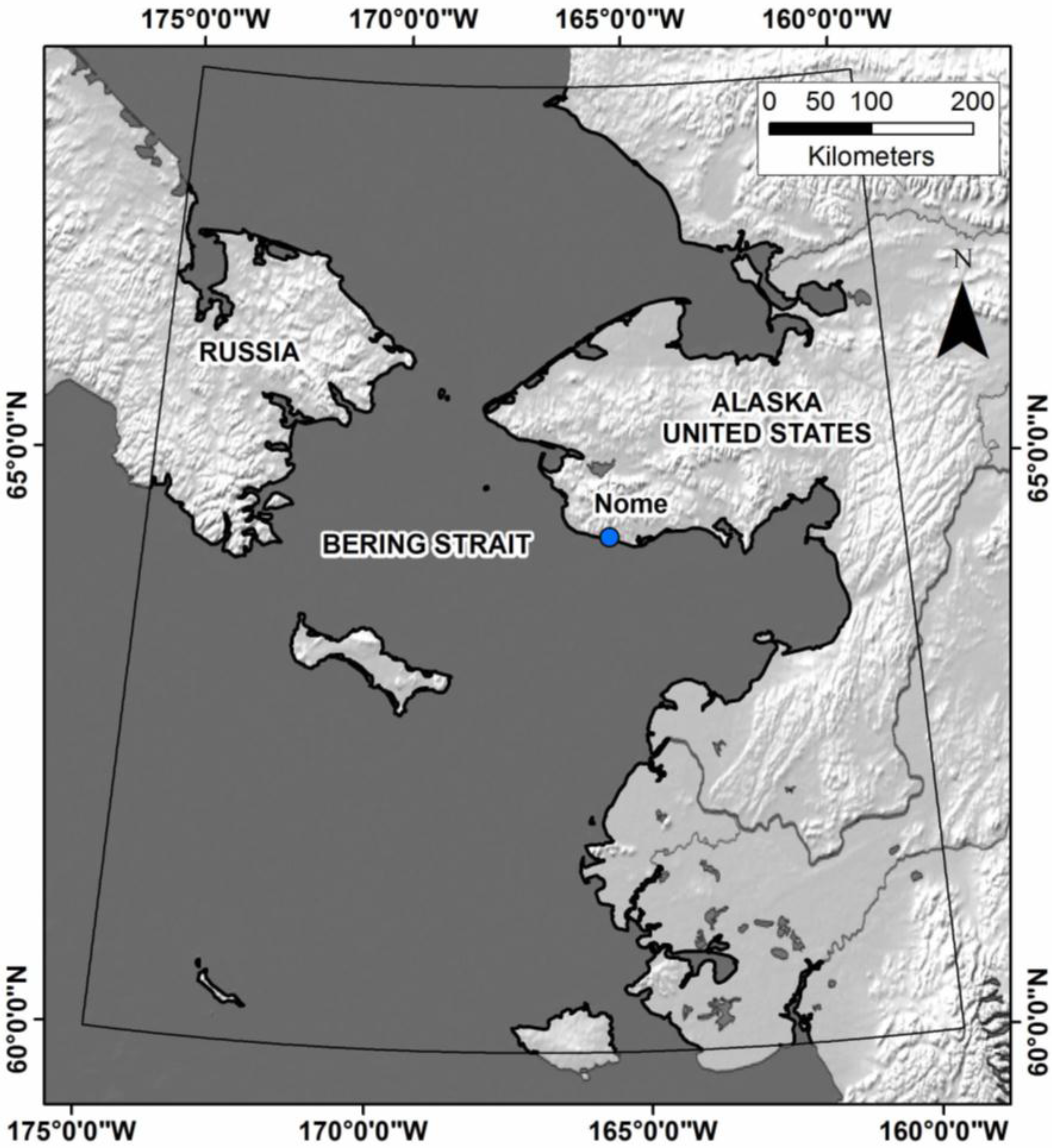
Establishing a scene model describing the study area is important in geospatial research applications [55,56]. The area of the current study encompasses the Bering Strait region and areas to its north and south between 159 and 175 degrees West longitude and between 60 and 68.5 degrees North latitude (Figure 1). The area typically experiences the formation and growth of sea ice beginning in October, generally centered along the coast, with ice thickening and expanding as temperatures drop and prevailing winds advect sea ice southward; the sea ice expands to maximum coverage by late March and begins a process of melting and retreating until the ocean is again exposed by late June [57]. Three major rivers (Yukon, Kobuk, and Noatak) and numerous smaller rivers and streams drain much of Interior Alaska into the Bering coastal zone. With northward ocean currents mixing Pacific Ocean-derived water with freshwater and nutrient runoff along the coast, combined with prevailing offshore winds of the Polar Easterlies, coastal upwelling processes help contribute to a bloom of plankton productivity during ice-diminished and ice-free months [58].
Figure 1. Map of Bering Strait study area.
Remotesensing 07 11863 g001

2.2. Predictor Variables

For an initial, exploratory study, spatial data were obtained for a collection of environmental variables in the Bering Strait. Some of the variables are associated with bearded seals in the literature (e.g., bathymetry, sea ice), others are recommended by indigenous hunters (e.g., bathymetry, distances from shore or anadromous fish streams [45]), while others are assumed to be of relative importance (e.g., bathymetric slope, sea surface temperature, chlorophyll concentration, etc.) for characterizing the habitat of bearded seals [59]. Environmental predictor variables used in this study are listed in Table 1.
Table 1. Environmental predictor variables used for bearded seal habitat suitability modeling, including data characteristics.
Environmental Data (Predictor Variables)Temporal RangeNative Spatial ResolutionData Source
Bathymetry (m)N/A0.833 kmSRTM30_Plus
Bathymetric slope (degrees)N/A4.167 kmSRTM30_Plus
Distance from coast (km)N/AN/AAlaska Geospatial Clearinghouse
Distance from anadromous streams (km)N/AN/AAlaska Geospatial Clearinghouse
Chlorophyll-a concentration (mg∙m3)2003–20124.167 kmNASA Ocean Biology Processing Group
Instantaneous Photosynthetically Available Radiation (Einstein m2∙sec)2003–20124.167 kmNASA Ocean Biology Processing Group
Photosynthetically Available Radiation (Einstein m2∙Day)2003–20124.167 kmNASA Ocean Biology Processing Group
Suspended solids (mol∙M3)2003–20124.167 kmNASA Ocean Biology Processing Group
Sea surface temperature (degrees Celsius)2003–20124.167 kmNASA Ocean Biology Processing Group
Sea ice (presence)2003–20123.607 kmNASA National Snow and Ice Data Center
Reflectance: Band 1 (R)2003–20120.986 kmNASA Land Products Group
Reflectance: Band 3 (B)2003–20120.986 kmNASA Land Products Group
Reflectance: Band 4 (G)2003–20120.986 kmNASA Land Products Group

2.3. Remotely-Sensed Data

Given such a large study area and the maritime environmental focus, selecting a sensor that provides the best compromise between temporal and spatial resolution and variety of data products is critical [60,61]. The Moderate-resolution Imaging Spectroradiometer (MODIS) instrument on board the NASA Terra and Aqua satellites provides near-daily global imaging data at resolutions ranging from 250 m to 1 km, using 36 spectral bands, resulting in many different raster products output by four major NASA research groups [62]. The data products selected from NASA research groups were eight-day composites produced natively at, or resampled to, a spatial resolution of 4 km where each grid cell value represents the maximum value observed for the cell over each eight-day time period, for the mid-June through October study period from 2003 to 2012. The mid-year window corresponds to the generally ice-free (or broken ice floes) period from Julian Day 137 to Julian Day 280. From the Land Products group (https://lpdaac.usgs.gov/), surface reflectance (SRF; MOD09) data for the visible wavelengths in Bands 4 (green), 3 (blue), and 1 (red) were acquired for tiles 9,2; 10,2; 11,2; and 12,2. Sea ice extent data for the Northern Hemisphere (SI; MOD29) was provided by the National Snow and Ice Data Center (http://nsidc.org/). The Ocean Color group (http://oceancolor.gsfc.nasa.gov) provided global scale data for chlorophyll-a concentration (CHL; MOD21), which has been found to predict habitat in other marine mammal studies [59], photosynthetically active and instantaneous photosynthetically active radiation (PAR, IPAR; MOD22), suspended solids as a measure of turbidity (PIC; MOD23), and sea surface temperature (SST; MOD28). Data voids in the Ocean Color products were in-filled using the Ocean Color group’s decadal climatology layers.

2.4. Other Spatial Data

The Alaska Geospatial Clearinghouse [63] provided vector data for the coastline at mean sea level (MSL) and hydrography for major rivers and river mouth locations. Distance grids with 4 km cell sizes were generated using Euclidean distances from the coastline vectors. A digital elevation model (DEM) containing terrestrial elevations above MSL and bathymetry below MSL was obtained from the SRTM 30 Plus repository [64]; the values of the layer “slope degrees” were generated from the DEM.

2.5. Response Variables

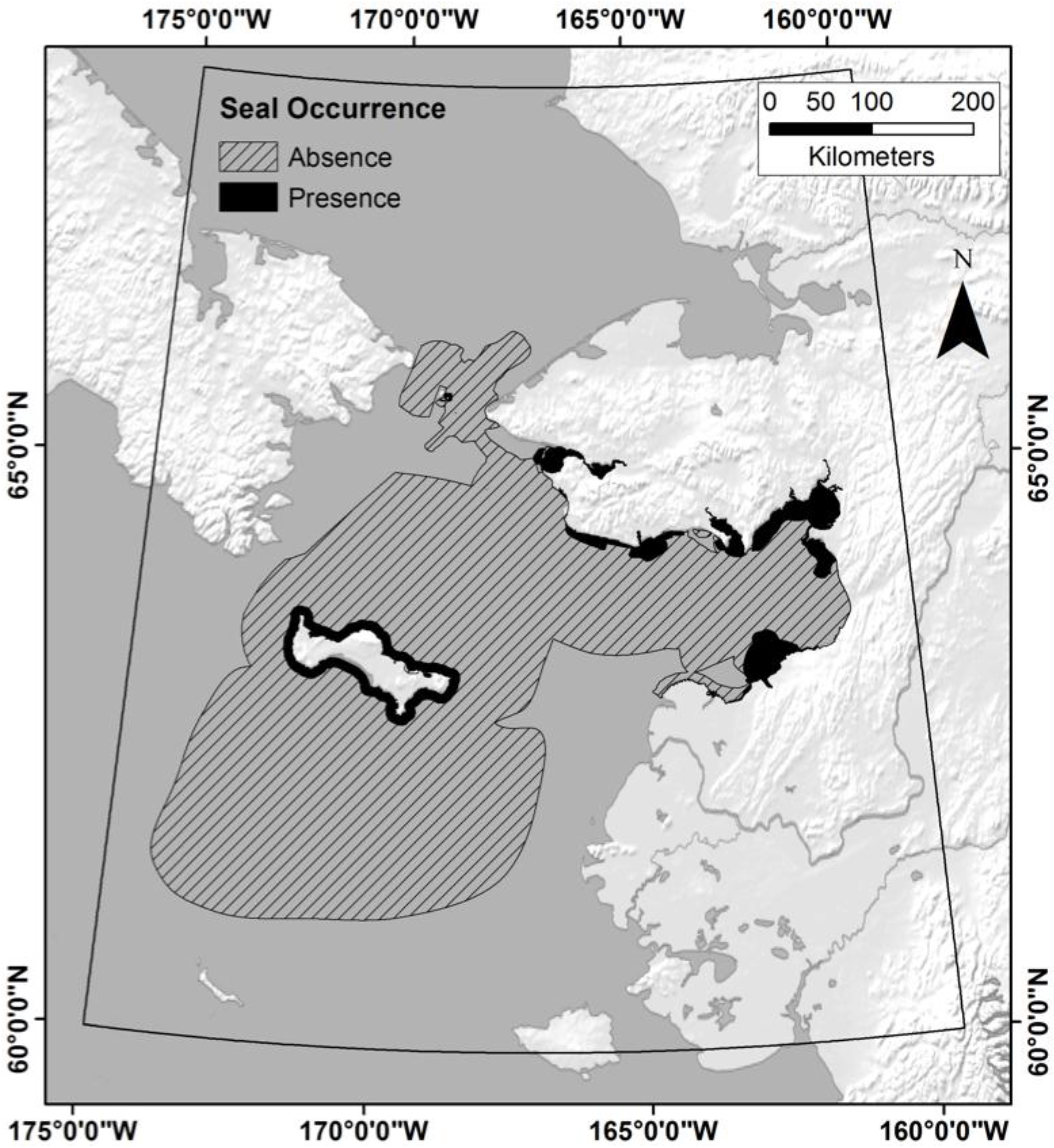
Although presence/absence data are preferred for species distribution and habitat suitability modeling, presence-only data has been successfully utilized [65,66,67]. TEK data was acquired by Kawerak from expert hunters and elders living in Bering Strait villages and includes seasonal maps of important hunting and search areas, areas where bearded seals concentrate, and the static and dynamic environmental characteristics of those areas that were considered important for hunting success [45]; areas that were no longer considered productive were excluded from final maps. TEK information was collected from indigenous hunters through interviews and focus groups, recorded in qualitative verbal responses and as locations marked on nautical charts, topographic maps, and other map products. Although all seasons were mapped, summer and fall habitat and harvest areas were extracted for this analysis. TEK polygons that indicated high concentrations of bearded seals for the summer or fall seasons were categorized as Good Habitat or Presence. The TEK data was presence-only data, but areas outside of those marked by hunters as good hunting or habitat area were categorized and treated as a type of pseudo-absence data for the purpose of this study (Figure 2).
Figure 2. TEK presence and pseudo-absence. Presence (black areas) includes some land surfaces where seals were present in rivers. Pseudo-absence is indicated by hatching and extends throughout Norton Sound and Bering Strait.
Remotesensing 07 11863 g002
Pseudo-absence data can be used in ecological studies when there is no data for true absences within a study area [67,68]. Including absence (or pseudo-absence) data has been found to increase the accuracy of species’ predictions compared to presence-only data [65]. Given that the entire study area is within the diving range of bearded seal and potentially habitat, a simple random point selection process was used within the TEK polygons that were categorized as pseudo-absence [69]. This differs somewhat from applications in terrestrial environments where habitat edges or ecotones are more well-known and can be more readily defined; for bearded seals, known edges are drop-offs such as the continental shelf where depths exceed their diving range, and such depths do not exist within the Bering Strait region.
Training and validation points were randomly generated within the presence and pseudo-absence polygons at a minimum distance of 4 km from each other to match the predictor variable cell size. One of the challenges of random point generation methods is identifying the optimal number of training and validation points and the minimum distance between points. To find the optimal number, we conducted multiple classifications using increasingly dense networks of points in order to examine the sensitivity of classification processes to the TEK data. The lowest-density trial data set generated included 30 training and 30 validation points (60 points total at the first level), and each subsequent trial data set progressed in size at 60-point increments for each new classification until reaching the final trial at 450 points for both training and validation (900 points total at the final level). Each trial evenly split the training and validation points between the two classes; e.g., the 60-point level included 15 random, independent training points representing the presence polygons, 15 training points representing pseudo-absence, 15 random, independent validation points for presence, and 15 validation points for pseudo-absence, for a total of 60 points. The sampling universe was 1222 potential cells for presence and 16,287 for pseudo-absence.

2.6. Data Extent and Pre-Processing

The greatest number of variables sharing a common projection, datum, and coarsest resolution came from the Ocean Color group; the Plate Caree [70,71] became the target projection for all other geospatial data. Data layers not already in the Plate Caree (an equidistant rectangular or geographic projection) were reprojected to that coordinate system, and all finer-scaled data were resampled to a common 4.1666667 km cell size. All data layers were subset to the study area’s latitude and longitude window.
Seasonal trend analyses (STA) were conducted on the time series MODIS products using Theil–Sen’s Estimator, a non-parametric approach that fits lines between all possible pairs of geographically coincident points in a time series for any given variable, and indicates whether the variable is increasing or decreasing in value and strength over time. Theil–Sen’s Estimator is a robust analysis technique, able to withstand up to 29% missing data and still produce reliable outputs [72,73,74,75]. Among its outputs are the mean of the data array, the median of all the slopes between pairwise coincident points throughout the time series, and the median for all of the intercepts in each time series. Prior to conducting Theil–Sen, the time series data were inspected, and although missing data were detected in the non-SST data across the study area, only in smaller, nearshore locations did they approach the 29% threshold. In order to be consistent with the SST data, which has no data voids [76], missing values in other time series data were infilled using Ocean Color decadal climatologies. Theil–Sen slope and intercept values for each time series predictor variable were calculated and used as input layers during the classification process; these are dynamic indicators of environmental processes that increase predictive and explanatory power of habitat modeling [77].
The time series predictor data was selected to match the TEK data seasonality of summer and fall (late June through October). The imagery and products represented a time span from May to October (Julian Day 137–280) with eight-day composite images and products.
Table 2. Environmental predictor variables by inclusion (+) or exclusion (−) from each analysis group, and the input band to the classification tree. Groupings include Theil–Sen (TS), Non-Theil–Sen (NTS), Sans Distance (−SD), and Sans Bathymetry (−SB) groups.
Raster Layer NameTSTS-SDTS-SD-SBNTSNTS-SDNTS-SD-SBInput Band
B01 TS Intercept+++1
B01 TS Slope+++2
B03 TS Intercept+++3
B03 TS Slope+++4
B04 TS Intercept+++5
B04 TS Slope+++6
Chlorophyll-a TS Intercept+++9
Chlorophyll-a TS Slope+++10
IPAR TS Intercept+++14
IPAR TS Slope+++15
PAR TS Intercept+++17
PAR TS Slope+++18
Sea Ice TS Intercept+++20
Sea Ice TS Slope+++21
Suspended Solids TS Intercept+++22
Suspended Solids TS Slope+++23
Sea Surface Temperature TS Intercept+++25
Sea Surface Temperature TS Slope+++26
Bathymetry Depth++++7
Bathymetry Slope++++8
Distance from Stream Outlets++12
Distance from Coast++13
Chlorophyll OC Climatology++++++11
IPAR OC Climatology++++++16
PAR OC Climatology++++++19
Suspended Solids OC Climatology++++++24
Sea Surface Temperature OC Climatology++++++27

2.7. Analysis

To develop a habitat suitability map, Classification Tree Analysis (CTA) was conducted [78,79,80] using GINI splitting rules with 10% pruning [81]. The major benefit of employing CTA, besides being non-parametric, is its transparent, “open box” approach that explicitly identifies which input layers (predictor variables) contribute to any particular classification output, and to which degree each input layer influenced the classification output [82]. In an exploratory study, it is important that the contributing variables are identified and known, as opposed to “black box” approaches that enshroud contributing variables (such as “hidden layers” in artificial neural networks) and only reveal the classification output [83]. Two major groupings of predictor variables were processed with CTA analyses and are presented in Table 2; the Theil–Sen (TS) group included the distance, bathymetry, OC climatologies, and STA input layers, while the non-Theil–Sen (NTS) omitted the STA input layers. For each CTA, a single tree was produced. Kappa statistics [84] were calculated for each CTA classification. The Theil–Sen and CTA analyses were conducted utilizing IDRISI software from Clark Labs.

3. Results

Test classifications indicated that the distance layers were a major driver of the classification results, constricting the output classification within the zones covered by TEK polygons. This was due to the TEK data being concentrated near coastal areas and mouths of rivers joining the waters of the Bering Strait and in areas closer to the settlements where hunters engage in subsistence hunting activities. This constriction was addressed by establishing a second CTA batch for each group that removed the distance layers (sans distance−SD). The secondary batch indicated that bathymetry was the next important environmental factor; however, bathymetry often reflects distance from shoreline. Thus, a third CTA batch (−SD−SB) removed the bathymetry layers and only used satellite-derived data products. Output layers from each individual CTA run classified bearded seal habitat as 1 and non-habitat as 0; each batch’s output layers were additively combined to construct model agreement map visualizations.

3.1. What Is the Optimal Number of Training and Validation Points to Use in a Classification?

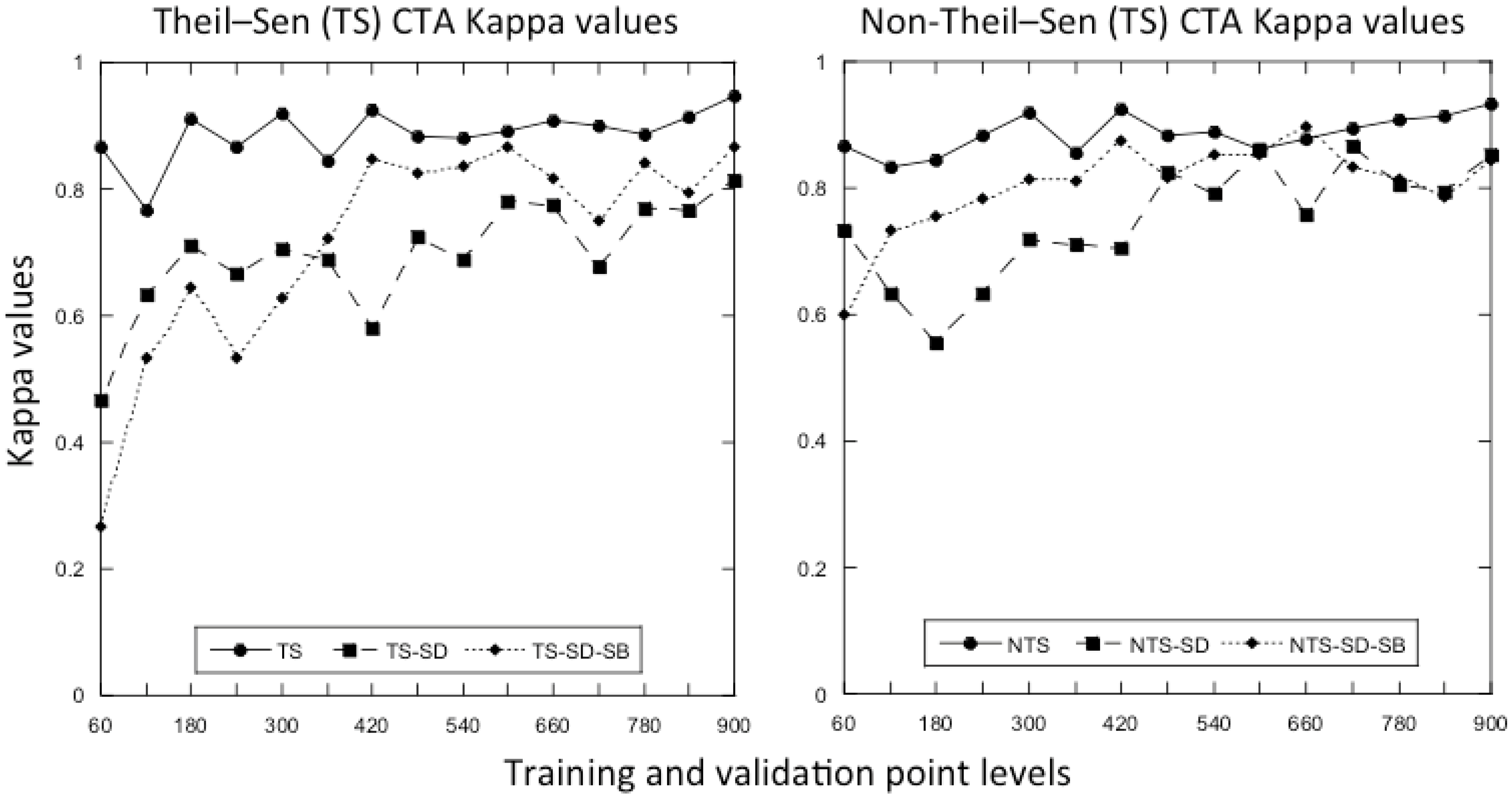
Kappa values for each classification run are presented in Figure 3. The CTA Kappas from TS and NTS series converge at the 480-point level (240 training and 240 validation), which may indicate the optimal point selection set for this study area and pixel size. The highest kappa value for both TS and NTS (0.883) was achieved for the runs that included all of the predictor variables for each series.

3.2. Which Predictor Variables Provide the Most Useful Information for Classification?
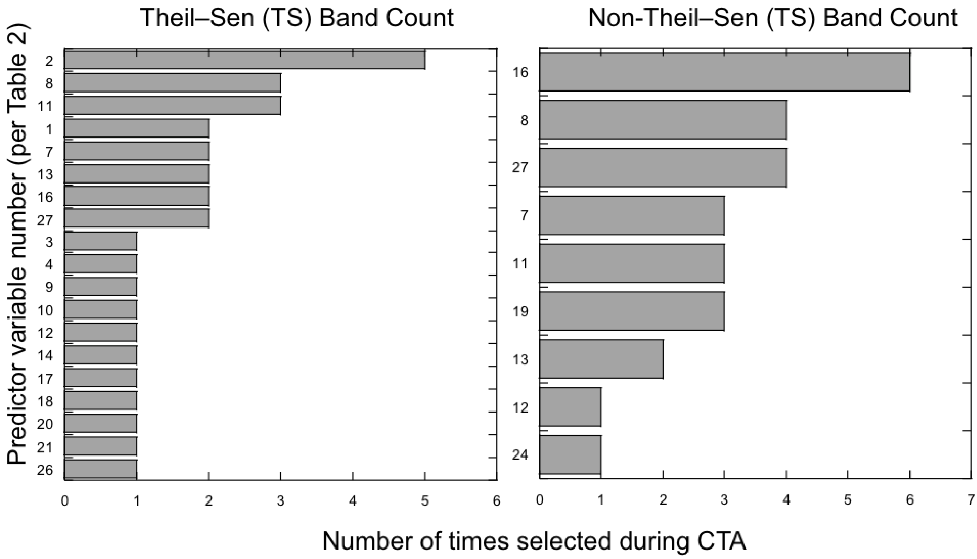
The frequency of input layer selection was summed from CTA output trees for each of the classification runs at the 480-point level, and is presented in Figure 4. For the Theil–Sen series of predictors, the TS Slope of MODIS B01 was selected five times, Bathymetric Slope was selected three times, Chlorophyll OC Climatology was selected three times, and 11 predictors from the array were each selected once (Sea Ice TS Intercept and Sea Ice TS Slope were among the predictors selected once each). For the non-Theil–Sen predictors, IPAR OC Climatology was selected six times, Bathymetric Slope and SST OC Climatology were selected four times each, and Distance from Stream Outlets and Suspended Solids were each selected once.
Figure 3. CTA Kappa values for Thiel–Sen (TS; left) and non-Thiel–Sen (NTS; right) analyses at the 480-point level, including iteration sans distance (SD) and sans bathymetry (SB). Kappa statistic values are plotted on the Y-axis, and the number of training and validation points for each trial is plotted on the X-axis by increments of 60.
Remotesensing 07 11863 g003
Figure 4. Band count histogram indicating how many times a particular band was selected within each of the six CTA batches conducted with 240 Training and 240 Validation points (480-point level). Bands are identified in Table 2.
Remotesensing 07 11863 g004

3.3. Does the Theil–Sen Time Series Data Improve the Accuracy of the Classification?
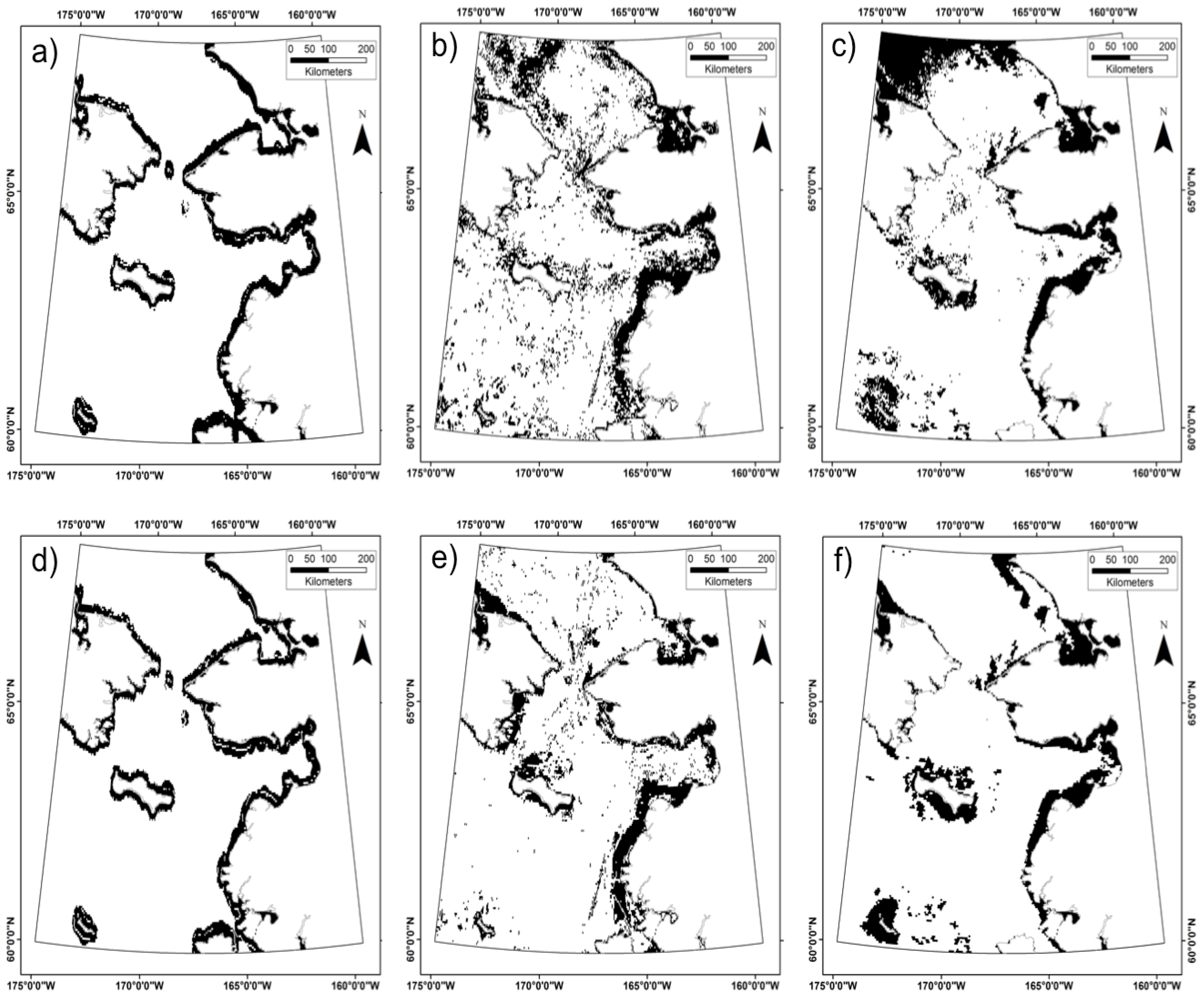
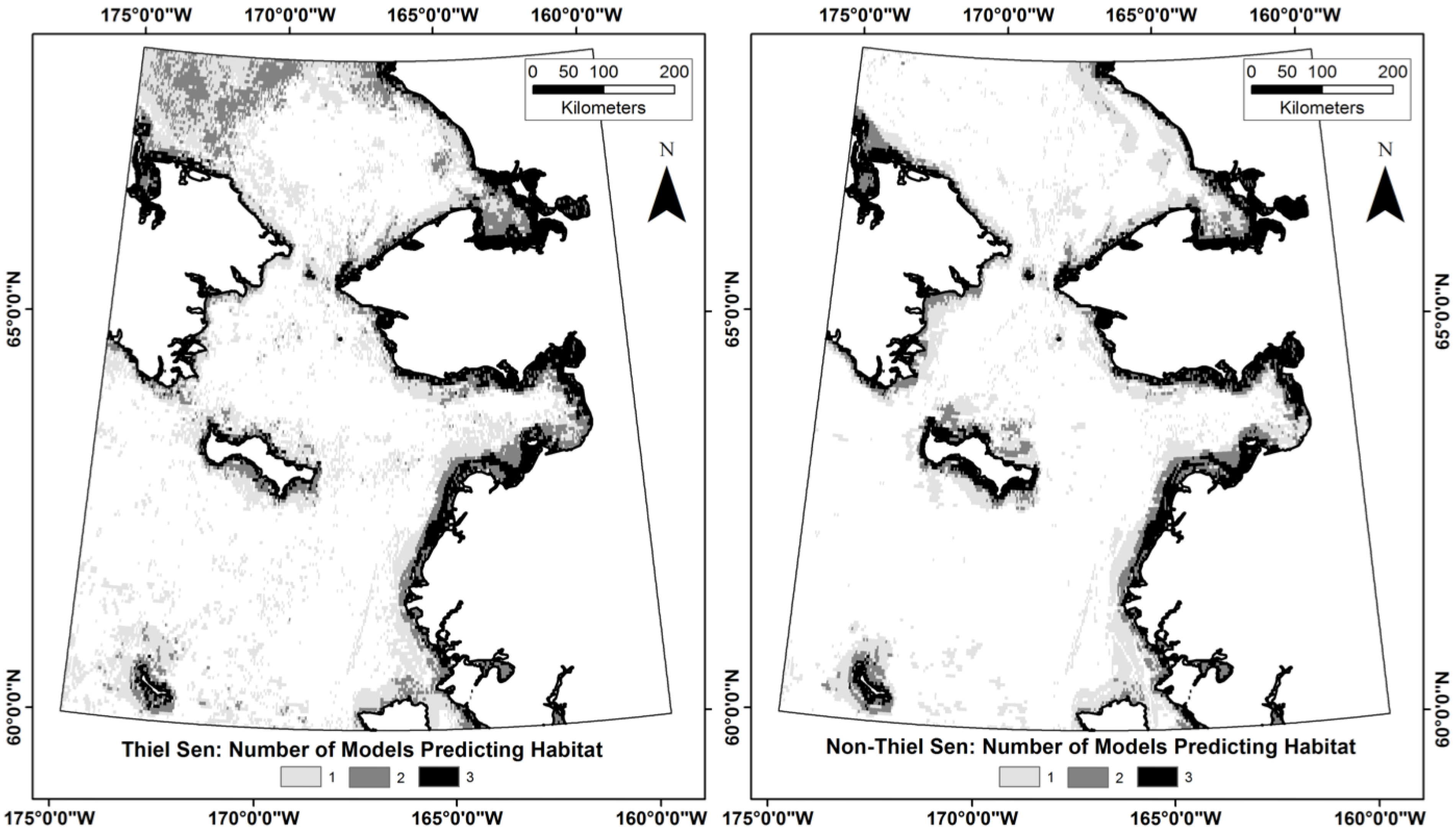
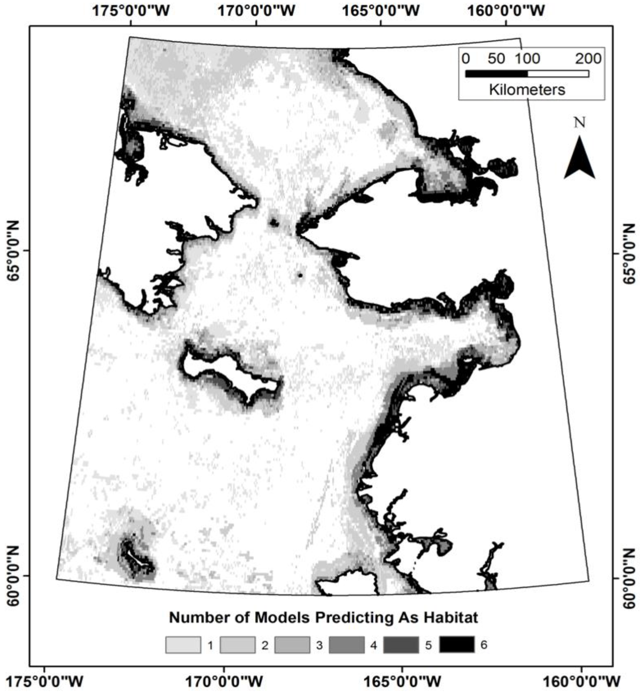
The frequency count data alone would seem to indicate that the Theil–Sen time series predictors are quite useful, perhaps to the point of excluding the non-Theil–Sen predictors. However, upon examining the output rasters for the two main CTA series, it appears that the NTS series produces similar results in areas that are nearer to the TEK presence training polygons. Figure 5 shows the individual habitat cell selections for each of the predictor variable sets, while Figure 6 shows composites of the TS and NTS series. Figure 7 is a composite of both TS and NTS series; all of these figures draw from the 480-point CTA analyses.
Figure 5. Initial habitat suitability maps. Theil–Sen (TS) maps: (a) all available inputs; (b) sans distance (SD); (c) sans distance, sans bathymetry (SD-SB). Non-Theil–Sen (NTS) maps: (d) all inputs except for Theil–Sen time series layers; (e) sans distance; (f) sans distance, sans bathymetry. All dark values are selected as bearded seal habitat for each classification.
Remotesensing 07 11863 g005
Figure 6. Composite habitat suitability maps for the Thiel–Sen (TS; left) and non-Thiel–Sen (NTS; right) analyses. The numbers 1, 2, and 3 indicate how many models within either the TS or NTS series selected a given pixel location as suitable habitat.
Remotesensing 07 11863 g006
Figure 7. Composite map showing the agreement between the six habitat suitability output maps at the 480-point modeling level.
Remotesensing 07 11863 g007
At the 480-point level where Kappa converges for both experimental series, there is variation in the number of predictor variables (bands) selected, the number of cells selected as suitable habitat, and the Kappa values for each CTA run. Table 3 shows that the TS series selects more cells as suitable habitat than NTS, and both TS and NTS series have maximum Kappa values of 0.883 when using the full set of environmental predictors assigned to each series. The −SD run for each series results in the greatest area selected as habitat combined with the highest number of bands selected during CTA analysis, but for the TS−SD run, it is also the lowest Kappa value. The −SD−SB run for each series selects less area as suitable habitat than −SD, and the TS series has a higher Kappa value than the NTS series. Overall, using the TS series of environmental predictors appears to improve classification accuracy and the TS predictors also result in larger areas being selected as suitable habitat.
Table 3. Number of bands included in the Classification Tree, number of cells classified as Presence (i.e., suitable habitat), and the Kappa value for the optimum classification produced for each variable group. Groups include Theil–Sen (TS) and non-Theil–Sen (NTS) variables, sans distance variables (−SD), and sans bathymetry variables (−SB) as defined in Table 2. Classifications produced at the 480-point (240 training and 240 validation) level.
TSTS-SDTS-SD-SBNTSNTS-SDNTS-SD-SB
Band Count715106129
Cells Selected817611,93911,525790984218403
Kappa0.8830.7250.8250.8830.8250.817

4. Discussion

4.1. Does TEK Function as a Reasonable Proxy for Western Scientific Data?

Western scientific observation is limited in remote areas such as the Bering Strait, especially when observations are also constrained by short seasonal opportunities to establish research posts and collect information. Existing maps of bearded seal habitat [47,49,50] essentially describe the spatial extent of depths within the bearded seal’s documented diving capacity, which includes the entirety of the Bering Strait and adjacent areas within the Bering and Chukchi Seas.
This study applies terrestrial habitat classification techniques to marine environments, building on the foundation of TEK data provided by Alaska Native hunters. The analyses selected subsets of the study area which are in turn subsets of established habitat maps for bearded seal in Bering Strait; these subset areas have similar characteristics to locations where bearded seal are known to have been harvested in subsistence hunts or locations where they were physically sighted (if not actually pursued by hunters). Using a more expansive selection of environmental predictor variables has provided insight into which portions of the Bering Sea might be more important or critical habitat zones for bearded seal populations within the more general habitat characteristic of maximum diving depth.

4.2. What Is the Optimal Number of Training and Validation Points to Use in a Classification?

The sensitivity analysis conducted in parallel with the CTA analysis showed that convergence occurred at 480 points, split into 240 for training and 240 for validation. For the area encompassed by the study, and the pixel resolution used for the input predictor variables, 480 points appears to be an optimal number for classification. The areal extent of the classifications also expanded at all sensitivity levels when the restrictive distance environmental variables were removed from the input set.
A potentially confounding factor with this study is that the training (1222) and validation (16,287) cell sets account for nearly half of the marine study area (45,694) prior to sampling. The Kappa statistic naturally improves and approaches 1.0 as the number of training and validation points increases at each experimental CTA level as shown in Figure 4. Directly related to this factor is that the 4-km pixel size aggregates and smooths environmental information in each data layer for both temporal and non-temporal geospatial data. Predictor variables at finer spatial resolutions, such as 250 m pixels, could provide more insight into the importance of the various predictors within the complex environment of Bering Strait.
The TEK information is also somewhat limited in its spatial extent (see Figure 2). Although the TEK polygons used to generate training and validation points for presence cover 19,552 km2 of area in the Bering Strait, those locations are still relatively close to the shorelines of the mainland and larger islands, and only on the U.S. side of the international border with Russia that bisect the Strait. The TEK information itself acts as a constraint on the habitat mapping since the nearshore environmental conditions are overrepresented compared to offshore environmental conditions as a function of where hunters preferentially seek their prey. However, interviews conducted with hunters and elders suggest that the nearshore environment is the preferred habitat of the seal during the summer and fall, as juveniles stay close to the easy feeding grounds afforded by river mouths, and adults conserve energy by staying close to the shore at a time when pack ice has receded far to the north [45].
As noted earlier, there are not clear demarcations for what constitutes habitat vs. non-habitat for bearded seals in the Bering Strait within the existing literature, except that the seals will not travel very far inland on dry land and have a maximum diving depth. The TEK observations of presence during the summer and fall seasons, which are limited to areas near participating communities, do not capture all the locations within Bering Strait where bearded seals exist and forage; using non-selected cells for pseudo-absence data does not mean that bearded seals are truly absent from those cells [65]. Rather, because the input TEK data were transformed as such, the subsequent classification of presence should be interpreted as the areas most favorable for higher concentrations of seals, while pseudo-absence includes less favorable habitat. These errors of omission [85], or false negatives, within the habitat classification analyses result in conservative predictions of bearded seal habitat in this study. However, the areas conservatively predicted as bearded seal habitat are the areas where the population is most concentrated during summer and fall seasons, and most critical to sustaining the population under a rapidly changing climate where sea ice continues to decrease.

4.3. Which Predictor Variables Provide the Most Information for Classification?

The initial test classifications revealed distance and bathymetry (a distance proxy) to wield the greatest predictive power. Once these were removed, using the remaining array of predictor variables for CTA analyses resulted in the Theil–Sen slope and intercept variables dominating when producing habitat maps, although it is notable that classifications from these variables still highlighted areas close to shore as being the most critical. Removing the Thiel–Sen variables and using only the NASA-produced Ocean Color climatologies produced habitat maps that were very similar to the Theil–Sen-based maps within the core of the study area (i.e., the region encompassing Norton Sound and St. Lawrence Island); both the TS and NTS environmental predictor series produced maps that matched the TEK data within the study area core. If an analyst has access to software that can produce the Theil–Sen predictor layers, the prediction results cover a broader geographic range; if the Theil–Sen layers are not producible, however, the reduced set of predictor layers appears to give comparable results near the core of the study area. No matter what input set of predictors was utilized, distance from shore and anadromous fish streams dominated the outcome classifications. This is both a product of the TEK input data, which highlighted the nearshore environment as being the most favorable hunting grounds, and it is consistent with observations about seal behavior from the Alaska Native contributors, who noted that seals favor the shoreline in summer and fall [45]. Subsistence hunters would travel further to more productive hunting grounds if necessary, but in summer and fall seasons find seals closer to the shore and bountiful runs of anadromous fish entering river mouths to spawn.
While ice is the focus of much climate change research in the Arctic, our focus here was on the summer and fall periods when the Bering Strait is ice-free. Thus, it is no surprise that the TS Sea Ice environmental layers were not important predictors for summer and fall seal habitat. Bearded seals are most highly associated with sea ice during the winter and spring seasons. However, since climate projections include longer ice-free periods in the Arctic [13], including the Bering Strait, it is particularly important to identify critical habitat areas during ice-free periods, and understand what ecological mechanisms drive preference of this habitat. As such, we were surprised that chlorophyll-a was not a strong predictor of habitat, as it has been found in other studies to predict suitable habitat for marine mammals because of its association with high plankton levels and the schools of fish that feed on plankton and serve as easy prey [59]. We posit that both the coarse spatial resolution of the data and the non-stationary nature of plankton (particularly relative to the stationary seal presence polygons) likely contributed to low selection of chlorophyll-a by the model. We also note that iPAR climatology was a strong predictor of seal habitat, and is also an indicator of phytoplankton [62]. By contrast, preference of nearshore habitat near anadromous fish streams highlights the importance of protecting these areas as commercialization of the region increases.

4.4. Is the Time Series Data Useful for the Classification Analysis?

The TS predictor set provides greater predicted habitat than the NTS predictor set at each of the three levels of analysis; the TS base level results in 3.4% more predicted habitat, the SD level results in 41.8% more, and the SD-SB level results in 37.2% more. The increased predicted habitat tends to occur further from the study area core, where the TEK presence polygons are located; the TS series appears to select more pixels in locations farther north in the Chukchi Sea and farther south in the Bering Sea. The NTS approach provides habitat selections similar to the TS selections in areas with closer proximity to the TEK polygons. Theil–Sen may be indicating areas of interest that could be more fully investigated at a later date with expanded predictor variable sets. A tradeoff may exist in terms of resources required for TS and NTS data; preparing NTS data may take a few days and select smaller areas as habitat, whereas TS data may take several weeks or months to pre-process prior to conducting analysis but select larger areas as habitat.

4.5. What Are the Utilities, Applications, and Limitations of the Model?
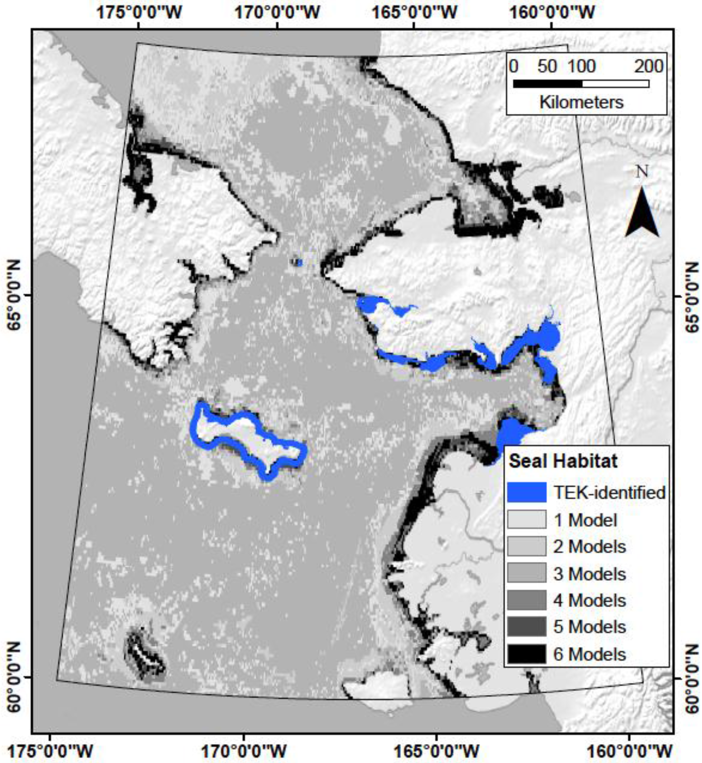
As with most modeling exercises, there are limitations to our conceptual approach. The low spatial resolution of remote sensing data available in the Arctic produces a loss in information that will hopefully be improved as new sensors are launched and multiscalar studies are undertaken. All remotely sensed data also inherently have error associated with atmospheric scattering, sensor sensitivity, and data post-processing (e.g., reprojection of data). There are currently no geospatially located Western scientific data on bearded seals in the region that would allow us to further validate the TEK-driven model, which may bring its utility into question. However, that is the exact reason for such a study as this—to utilize non-traditional information in a modern modeling framework when Western scientific data don’t yet exist.
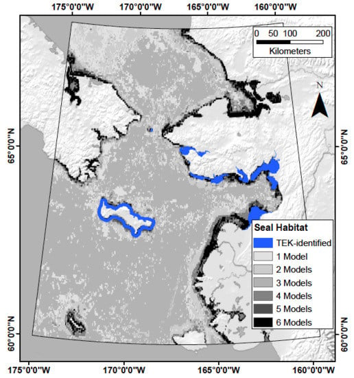
Figure 8. Composite map showing the agreement between the six habitat suitability output maps at the 480-point modeling level and the training polygons of known seal presence derived from Traditional Ecological Knowledge (TEK).
Remotesensing 07 11863 g008
This synthesis of indigenous knowledge and published Western science demonstrates that the TEK of Alaska Native hunters can be transformed into digital training and validation information and effectively used in geospatial modeling of marine mammal habitat. In a remote region where Western science data are difficult to acquire, the TEK of indigenous people who subsist on the marine mammals provided a source of environmental information on bearded seal habitat. A limitation of this information was that the spatial extent of the documented seal presence was limited to hunting grounds near villages. By using TEK data in a CTA framework, however, we were able to highlight which predictors were most critical for seal habitat and map additional likely habitat around the region. Because we suggest our map was likely a conservative estimate of habitat, areas identified by multiple models that are outside of the TEK presence polygon should be considered to have high potential as bearded seal habitat. These include the shorelines outside of the TEK presence areas near Nome, Alaska, and the open ocean areas outside of the near-island buffers (Figure 8). The extended offshore areas around St. Lawrence Island in particular point to the value of the MODIS-derived predictor variables, as these pixels would not be selected from bathymetry and shoreline alone. Since these areas exhibit a high likelihood of being habitat, they could be prioritized for observation during future data collection surveys, and would potentially be a top priority for protection measures as policy negotiations ensue.

5. Conclusions

This study presented a novel framework for integrating Traditional Ecological Knowledge (TEK) with existing, published modeling approaches that usually utilize Western science observations, and applied existing habitat classification and analysis techniques to an Arctic marine environment; the Bering Strait. It transformed TEK acquired from interviews and focus groups with Alaska Native hunters and elders into spatial representations of bearded seal presence and pseudo-absence, and then utilized a classification tree methodology for classifying additional potential seal habitat. Results showed that Kappa values were highest (κ = 0.883) when using 480 randomly-selected training and validation points, and distance from shore and bathymetry were the dominant drivers of the initial seal habitat models. A third model excluding these two predictor variables selected higher phytoplankton concentrations as the best predictor. The resulting seal habitat suitability map highlighted regions outside of the TEK-identified seal presence areas that are likely key areas for bearded seals.
This study introduces a novel approach for incorporating a non-Western science source of training and validation data to habitat classification. Future research in this arena should seek both finer scale remotely sensed data and more observations of bearded seal habitat use, from both Western scientific studies and communities that did not participate in the TEK project. This study provides an objective, replicable methodological framework that can be applied in conjunction with or in the absence of Western science data, particularly when time and resources are limited and policy decisions rely on the best available science.

Acknowledgments

We thank Kawerak, Inc. for sharing data from their Ice Seal and Walrus project, and the 82 local experts who contributed their knowledge, and the nine participating tribes from the Bering Strait region who contributed their knowledge to that project. Julie Raymond-Yakoubian obtained grant funding for the Ice Seal and Walrus Project, provided expert consultation and collaboration throughout the project, and reviewed this manuscript. Funding support for Olsen and Kolden came from NASA Award NNX10AT77A. Funding support for Kawerak, Inc. data collection and Gadamus came from the Oak Foundation award No. 2010-OUSA-073, the National Science Foundation award No. ARC-1023686, and the National Fish and Wildlife Foundation award No. 2010-0061-004. Any opinions, findings, conclusions, or recommendations expressed in this publication are those of the authors and do not necessarily reflect the views of the funders or project partners.

Author Contributions

All authors designed the research, interpreted results, and contributed to manuscript writing. Patrick Olsen acquired and processed satellite and ancillary data, conducted data analysis, and developed figures and tables. Crystal Kolden supervised the analysis, and conducted revisions. Lily Gadamus led the Kawerak Ice Seal and Walrus TEK project (which included research design, data collection, and analysis), and supervised the integration of TEK data into the analysis.

Conflicts of Interest

The authors declare no conflict of interest.

References

  1. Ackerman, R.E. Early maritime traditions in the Bering, Chukchi, and east Siberian seas. Arct. Anthropol. 1998, 35, 247–262. [Google Scholar]
  2. Gadamus, L. Linkages between human health and ocean health: A participatory climate change vulnerability assessment for marine mammal harvesters. Int. J. Circumpolar Health 2013, 72, 20715. [Google Scholar] [CrossRef] [PubMed] [Green Version]
  3. Ahmasuk, A.; Trigg, E.; Magdanz, J.; Robbins, B. A Comprehensive Subsistence Use Study of the Bering Strait Region; Kawerak, Inc.: Nome, AK, USA, 2008. [Google Scholar]
  4. Moore, S.E.; Huntington, H.P. Arctic marine mammals and climate change: Impacts and resilience. Ecol. Appl. 2008, 18, S157–S165. [Google Scholar] [CrossRef] [PubMed]
  5. Grebmeier, J.M. Shifting patterns of life in the pacific arctic and sub-arctic seas. Annu. Rev. Mar. Sci. 2012, 4, 63–78. [Google Scholar] [CrossRef] [PubMed]
  6. Laidre, K.L.; Stirling, I.; Lowry, L.F.; Wiig, O.; Heide-Jorgensen, M.P.; Ferguson, S.H. Quantifying the sensitivity of arctic marine mammals to climate-induced habitat change. Ecol. Appl. 2008, 18, S97–S125. [Google Scholar] [CrossRef] [PubMed]
  7. Burek, A.; Gulland, F.M.D.; O’Hara, T.M. Effects of climate change on arctic marine mammal health. Ecol. Appl. 2008, 18, S126–S134. [Google Scholar] [CrossRef] [PubMed]
  8. Stafford, K. Anthropogenic Sound and Marine Mammals in the Arctic; The Pew Charitable Trusts: Seattle, WA, USA, 2013. [Google Scholar]
  9. Sackinger, W.M.; Jeffries, M.O. Symposium on noise and marine mammals. In Port and Ocean Engineering under Arctic Conditions; Sackinger, W.M., Jeffries, M.O., Eds.; The Geophysical Institute, University of Alaska Fairbanks: Anchorage, AK, USA, 1988; p. 131. [Google Scholar]
  10. Huntington, H.P. A preliminary assessment of threats to arctic marine mammals and their conservation in the coming decades. Mar. Policy 2009, 33, 77–82. [Google Scholar] [CrossRef]
  11. Maslowski, W.; Kinney, J.C.; Higgins, M.; Roberts, A. The future of arctic sea ice. Annu. Rev. Earth Planet. Sci. 2012, 40, 625–654. [Google Scholar] [CrossRef]
  12. Kwok, R.; Untersteiner, N. The thinning of arctic sea ice. Phys. Today 2011, 64, 36–41. [Google Scholar] [CrossRef]
  13. Douglas, D.C. Arctic Sea Ice Decline: Projected Changes in Timing and Extent of Sea Ice in the Bering and Chukchi Seas; U.S. Geological Survey: Reston, VA, USA, 2010. [Google Scholar]
  14. Walsh, J.E.; Overland, J.E.; Groisman, P.Y.; Rudolf, B. Ongoing climate change in the arctic. AMBIO 2011, 40, 6–16. [Google Scholar] [CrossRef]
  15. Kwok, R.; Rothrock, D.A. Decline in arctic sea ice thickness from submarine and icesat records: 1958–2008. Geophys. Res. Lett. 2009, 36, L15501. [Google Scholar] [CrossRef]
  16. Wang, M.; Overland, J.E.; Stabeno, P. Future climate of the Bering and Chukchi seas projected by global climate models. Deep Sea Res. II: Top. Stud. Oceanogr. 2012, 65–70, 46–57. [Google Scholar] [CrossRef]
  17. Arctic Council. Arctic Marine Shipping Assessment 2009 Report, 2nd ed.; Arctic Council: Tromsø, Norway, 2009. [Google Scholar]
  18. Brigham, L.; Smith, E. The Future of Arctic Marine Navigation in Mid-Century; Arctic Council: Tromsø, Norway, 2008. [Google Scholar]
  19. Kitagawa, H. Arctic routing: Challenges and opportunities. WMU J. Marit. Aff. 2008, 7, 485–503. [Google Scholar] [CrossRef]
  20. Stephenson, S.R.; Smith, L.C.; Brigham, L.W.; Agnew, J.A. Projected 21st-century changes to arctic marine access. Clim. Chang. 2013, 118, 885–899. [Google Scholar] [CrossRef]
  21. Conley, H.; Pumphrey, D.L. Arctic Economics in the 21st Century: The Benefits and Costs of Cold; Center for Strategic & International Studies: Washington, DC, USA, 2013. [Google Scholar]
  22. Wolfe, R.J.; Walker, R.J. Subsistence economies in Alaska: Productivity, geography, and development impacts. Arct. Anthropol. 1987, 24, 56–81. [Google Scholar]
  23. Ackerman, R.E. Settlements and sea mammal hunting in the Bering-Chukchi sea region. Arct. Anthropol. 1988, 25, 52–79. [Google Scholar]
  24. Huntington, H.P.; Sookiayak, C. Traditional Ecological Knowledge of Seals in Norton Bay, Alaska; Elim-Shaktoolik-Koyuk Marine Mammal Commission: Eagle River, AK, USA, 2000. [Google Scholar]
  25. Katsanevakis, S.; Stelzenmuller, V.; South, A.; Sorensen, T.K.; Jones, P.J.S.; Kerr, S.; Badalamenti, F.; Anagnostou, C.; Breen, P.; Chust, G.; et al. Ecosystem-based marine spatial management: Review of concepts, policies, tools, and critical issues. Ocean. Coast. Manag. 2011, 54, 807–820. [Google Scholar] [CrossRef]
  26. Kaplan, D.M.; Planes, S.; Fauvelot, C.; Brochier, T.; Lett, C.; Bodin, N.; Le Loc’h, F.; Tremblay, Y.; Georges, J.-Y. New tools for the spatial management of living marine resources. Curr. Opin. Environ. Sustain. 2010, 2, 88–93. [Google Scholar] [CrossRef]
  27. Wilson, C.D.; Roberts, D.; Reid, N. Applying species distribution modelling to identify areas of high conservation value for endangered species: A case study using Margaritifera margaritifera (L.). Biol. Conserv. 2011, 144, 821–829. [Google Scholar] [CrossRef]
  28. Schofield, G.; Scott, R.; Dimadi, A.; Fossette, S.; Katselidis, K.A.; Koutsoubas, D.; Lilley, M.K.S.; Pantis, J.D.; Karagouni, A.D.; Hays, G.C. Evidence-based marine protected area planning for a highly mobile endangered marine vertebrate. Biol. Conserv. 2013, 161, 101–109. [Google Scholar] [CrossRef]
  29. Schmelzer, I. Seals and seascapes: Covariation in Hawaiian monk seal subpopulations and the oceanic landscape of the Hawaiian archipelago. J. Biogeogr. 2000, 27, 901–914. [Google Scholar] [CrossRef]
  30. Boyd, D.S.; Foody, G.M. An overview of recent remote sensing and GIS-based research in ecological informatics. Ecol. Inform. 2011, 6, 25–36. [Google Scholar] [CrossRef]
  31. Guisan, A.; Zimmermann, N. Predictive habitat distribution models in ecology. Ecol. Model. 2000, 135, 147–186. [Google Scholar] [CrossRef]
  32. Elith, J.; Leathwick, J.R. Species distribution models: Ecological explanation and prediction across space and time. Annu. Rev. Ecol. Evol. Syst. 2009, 40, 677–697. [Google Scholar] [CrossRef]
  33. Guisan, A.; Thuiller, W. Predicting species distribution: Offering more than simple habitat models. Ecol. Lett. 2005, 8, 993–1009. [Google Scholar] [CrossRef]
  34. Miller, J. Species distribution modeling. Geogr. Compass 2010, 4, 490–509. [Google Scholar] [CrossRef]
  35. Dobrowski, S.Z.; Safford, H.D.; Cheng, Y.B.; Ustin, S.L. Mapping mountain vegetation using species distribution modeling, image-based texture analysis, and object-based classification. Appl. Veg. Sci. 2008, 11, 499–508. [Google Scholar] [CrossRef]
  36. Treitz, P.; Howarth, P. Integrating spectral, spatial, and terrain variables for forest ecosystem classification. Photogramm. Eng. Remote Sens. 2000, 66, 305–317. [Google Scholar]
  37. Vogelmann, J.E.; Sohl, T.; Howard, S.M. Regional characterization of land cover using multiple sources of data. Photogramm. Eng. Remote Sens. 1998, 64, 45–57. [Google Scholar]
  38. Mumby, P.; Green, E.; Edwards, A.; Clark, C. Coral reef habitat mapping: How much detail can remote sensing provide? Mar. Biol. 1997, 130, 193–202. [Google Scholar] [CrossRef]
  39. Kachelriess, D.; Wegmann, M.; Gollock, M.; Pettorelli, N. The application of remote sensing for marine protected area management. Ecol. Indic. 2014, 36, 169–177. [Google Scholar] [CrossRef]
  40. Azzellino, A.; Panigada, S.; Landredi, C.; Zanardelli, M.; Airoldi, S.; Notarbartolo di Sciara, G. Predictive habitat models for managing marine areas: Spatial and temporal distribution of marine mammals within the Pelagos sanctuary (northwestern Mediterranean sea). Ocean. Coast. Manag. 2012, 67, 63–74. [Google Scholar] [CrossRef]
  41. Polovina, J.; Howell, E.; Kobayashi, D.; Seki, M. The transition zone chlorophyll front, a dynamic global feature defining migration and forage habitat for marine resources. Prog. Oceanogr. 2001, 49, 461–483. [Google Scholar] [CrossRef]
  42. Mishra, D.; Narumalani, S.; Rundquist, D.; Lawson, M. Benthic habitat mapping in tropical marine environments using Quickbird multispectral data. Photogramm. Eng. Remote Sens. 2006, 72, 1037–1048. [Google Scholar] [CrossRef]
  43. Alaska Department of Fish and Game. Ice Seal Movement and Habitat Use Study. Available online: http://www.adfg.alaska.gov/index.cfm?adfg=marinemammalprogram.icesealmovements (accessed on 10 August 2015).
  44. Kawerak Inc. Traditions of Respect: Traditional Knowledge from Kawerak’s Ice Seal and Walrus Project; Kawerak Social Science Program: Nome, AK, USA, 2013. [Google Scholar]
  45. Kawerak Inc. Seal and Walrus Harvest and Habitat Areas for Nine Bering Strait Region Communities; Kawerak Social Science Program: Nome, AK, USA, 2013. [Google Scholar]
  46. National Marine Fisheries Service (NMFS). Endangered and Threatened Species; Threatened Status for the Beringia and Okhotsk Distinct Population Segments of the Erignathus Barbatus Nauticus Subspecies of the Bearded Seal; NMFS: Washington, DC, USA, 2012; Volume 77, pp. 76740–76768. [Google Scholar]
  47. Burns, J.J. Bearded sealErignathus barbatus. In Handbook of Marine Mammals; Ridgway, S.H., Harrison, R.J., Eds.; Academic Press, Inc.: New York, NY, USA, 1981; Volume 2, pp. 145–170. [Google Scholar]
  48. Quakenbush, L.; Citta, J.; Crawford, J. Biology of the Bearded Seal (Erignathus barbatus) in Alaska, 1961–2009; Arctic Marine Mammal Program: Fairbanks, AK, USA, 2011; p. 71. [Google Scholar]
  49. Cameron, M.F.; Bengston, J.L.; Boveng, P.L.; Jansen, J.K.; Kelly, B.P.; Dahle, S.P.; Logerwell, E.A.; Overland, J.E.; Sabine, C.L.; Waring, G.T.; et al. Status Review of the Bearded Seal (Erignathus barbatus); U.S. Department of Commerce: Washington, DC, USA, 2010. [Google Scholar]
  50. National Marine Fisheries Service (NMFS). Bearded Seal Range; Office of Protected Resources-NMFS: Silver Spring, MD, USA, 2009. [Google Scholar]
  51. Ver Hoef, J.M.; Cameron, M.F.; Boveng, P.L.; London, J.M.; Moreland, E.E. A spatial hierarchical model for abundance of three ice-associated seal species in the eastern Bering sea. Stat. Methodol. 2014, 17, 46–66. [Google Scholar] [CrossRef]
  52. Berkes, F.; Colding, J.; Folke, C. Rediscovery of traditional ecological knowledge as adaptive management. Ecol. Appl. 2000, 10, 1251–1262. [Google Scholar] [CrossRef]
  53. Giddings, J.L. Cultural continuities of Eskimos. Am. Antiq. 1961, 27, 155–173. [Google Scholar] [CrossRef]
  54. Dumond, D.E. The norton tradition. Arct. Anthropol. 2000, 37, 1–22. [Google Scholar]
  55. Strahler, A.H.; Woodcock, C.E.; Smith, J.A. On the nature of models in remote sensing. Remote Sens. Environ. 1986, 20, 121–139. [Google Scholar] [CrossRef]
  56. Woodcock, C.E.; Strahler, A.H. The factor of scale in remote sensing. Remote Sens. Environ. 1987, 21, 311–332. [Google Scholar] [CrossRef]
  57. Pease, C.H.; Schoenberg, S.A.; Overland, J.E. A Climatology of the Bering Sea and Its Relation to the Sea Ice Extent; Pacific Marine Environmental Laboratory: Seattle, WA, USA, 1982. [Google Scholar]
  58. Loughlin, T.R.; Sukhanova, I.N.; Sinclair, E.H.; Ferrero, R.C. Summary of biology and ecosystem dynamics in the Bering sea. In Ak-sg-99–03: Dynamics of the Bering Sea; Loughlin, T.R., Ohtani, K., Eds.; University of Alaska Sea Grant, North Pacific Marine Science Organization (PICES): Fairbanks, AK, USA, 1999; pp. 387–407. [Google Scholar]
  59. Pittman, S.J.; Costa, B. Linking cetaceans to their environment: Spatial data acquisition, digital processing and predictive modeling for marine spatial planning in the Northwest Atlantic. In Spatial Complexity, Informatics, and Wildlife Conservation; Cushman, S.A., Huettmann, F., Eds.; Springer: New York, NY, USA, 2010; pp. 387–408. [Google Scholar]
  60. Phinn, S.R. A framework for selecting appropriate remotely sensed data dimensions for environmental monitoring and management. Int. J. Remote Sens. 1998, 19, 3457–3463. [Google Scholar] [CrossRef]
  61. Phinn, S.R.; Stow, D.A.; Franklin, J.; Mertes, L.A.K.; Michaelsen, J. Remotely sensed data for ecosystem analyses: Combining hierarchy theory and scene models. Environ. Manag. 2003, 31, 429–441. [Google Scholar] [CrossRef] [PubMed]
  62. NASA. MODIS Overview. Available online: https://lpdaac.usgs.gov/products/modis_overview (accessed on 15 August 2015).
  63. State of Alaska. Alaska State Geo-Spatial Data Clearinghouse. Available online: http://www.asgdc.state.ak.us/ (accessed on 12 April 2013).
  64. Becker, J.J.; Sandwell, D.T.; Smith, W.H.F.; Braud, J.; Binder, B.; Depner, J.; Fabre, D.; Factor, J.; Ingalls, S.; Kim, S.-H.; et al. Global bathymetry and elevation data at 30 arc seconds resolution: Srtm30_plus. Mar. Geod. 2009, 32, 355–371. [Google Scholar] [CrossRef]
  65. Brotons, L.; Thuiller, W.; Araujo, M.B.; Hirzel, A.H. Presence-absence versus presence-only modelling methods for predicting bird habitat suitability. Ecography 2004, 27, 437–448. [Google Scholar] [CrossRef]
  66. Hirzel, A.H.; Le Lay, G.; Helfer, V.; Randin, C.; Guisan, A. Evaluating the ability of habitat suitability models to predict species presences. Ecol. Modell. 2006, 199, 142–152. [Google Scholar] [CrossRef]
  67. Sequeira, A.; Mellin, C.; Rowat, D.; Meekan, M.G.; Bradshaw, C.J.A. Ocean-scale prediction of whale shark distribution. Divers. Distrib. 2012, 18, 504–518. [Google Scholar] [CrossRef]
  68. Wisz, M.S.; Guisan, A. Do pseudo-absence selection strategies influence species distribution models and their predictions? An information-theoretic approach based on simulated data. BMC Ecol. 2009, 9, 8. [Google Scholar] [CrossRef] [PubMed]
  69. Stokland, J.N.; Halvorsen, R.; Stoa, B. Species distribution modelling—Effect of design and sample size of pseudo-absence observations. Ecol. Modell. 2011, 222, 1800–1809. [Google Scholar] [CrossRef]
  70. Fenna, D. Cartographic Science: A Compendium of Map Projections, with Derivations; CRC Press: Boca Raton, FL, USA, 2007. [Google Scholar]
  71. Snyder, J.P. Flattening the Earth: Two Thousand Years of Map Projections; The University of Chicago Press: Chicago, IL, USA, 1993. [Google Scholar]
  72. Eastman, J.R.; Sangermano, F.; Ghimire, B.; Zhu, H.; Chen, H.; Neeti, N.; Cai, Y.; Machado, E.A.; Crema, S.C. Seasonal trend analysis of image time series. Int. J. Remote Sens. 2009, 30, 2721–2726. [Google Scholar] [CrossRef]
  73. Neeti, N.; Eastman, J.R. A contextual Mann-Kendall approach for the assessment of trend significance in image time series. Trans. GIS 2011, 15, 599–611. [Google Scholar] [CrossRef]
  74. Fernandes, R.; Leblanc, S.G. Parametric (modified least squares) and non-parametric (Theil–Sen) linear regressions for predicting biophysical parameters in the presence of measurement errors. Remote Sens. Environ. 2005, 95, 303–316. [Google Scholar] [CrossRef]
  75. Eastman, J.R.; Sangermano, F.; Machado, E.A.; Rogan, J.; Anyamba, A. Global trends in seasonality of normalized difference vegetation index (NDVI), 1982–2011. Remote Sens. 2013, 5, 4799–4818. [Google Scholar] [CrossRef]
  76. Campbell, J.W.; Blaisdell, J.M.; Darzi, M. SeaWiFS Data Products: Spatial and Temporal Binning Algorithms; SeaWiFS Technical Report Series; Goddard Space Flight Center: Greenbelt, MD, USA, 1995. [Google Scholar]
  77. Austin, M.P. Spatial prediction of species distribution: An interface between ecological theory and statistical modelling. Ecol. Modell. 2002, 157, 101–118. [Google Scholar] [CrossRef]
  78. Miller, J.; Franklin, J. Modeling the distribution of four vegetation alliances using generalized linear models and classification trees with spatial dependence. Ecol. Modell. 2002, 157, 227–247. [Google Scholar] [CrossRef]
  79. De’Ath, G.; Fabribius, K.E. Classification and regression trees: A powerful yet simple technique for ecological data analysis. Ecology 2000, 81, 3178–3192. [Google Scholar] [CrossRef]
  80. Loh, W.-Y. Classification and regression trees. WIREs Data Min. Knowl. Discov. 2011, 1, 14–23. [Google Scholar] [CrossRef]
  81. Zambon, M.; Lawrence, R.; Bunn, A.; Powell, S. Effect of alternative splitting rules on image processing using classification tree analysis. Photogramm. Eng. Remote Sens. 2006, 72, 25–30. [Google Scholar] [CrossRef]
  82. Lawrence, R.L.; Wright, A. Rule-based classification systems using classification and regression tree (CART) analysis. Photogramm. Eng. Remote Sens. 2001, 67, 1137–1142. [Google Scholar]
  83. Qiu, F.; Jensen, J.R. Opening the black box of neural networks for remote sensing image classification. Int. J. Remote Sens. 2004, 25, 1749–1768. [Google Scholar] [CrossRef]
  84. Congalton, R.G. Accuracy assessment and validation of remotely sensed and other spatial information. Int. J. Wildland Fire 2001, 10, 321–328. [Google Scholar] [CrossRef]
  85. Congalton, R.G.; Green, K. Assessing the Accuracy of Remotely Sensed Data: Principles and Practices, 2nd ed.; CRC Press: Boca Raton, FL, USA, 2009. [Google Scholar]