Article

Dual-Antenna Terrestrial Laser Scanner Georeferencing Using Auxiliary Photogrammetric Observations

Geomatics Program, School of Forest Resources & Conservation, University of Florida, 304 Reed Lab, Gainesville, FL 32611-0565, USA
*
Author to whom correspondence should be addressed.
Remote Sens. 2015, 7(9), 11621-11638; https://doi.org/10.3390/rs70911621
Submission received: 19 June 2015 / Revised: 10 August 2015 / Accepted: 2 September 2015 / Published: 11 September 2015

Abstract

:
Terrestrial laser scanning typically requires the use of artificial targets for registration and georeferencing the data. This equipment can be burdensome to transport and set up, representing expense in both time and labor. Environmental factors such as terrain can sometimes make target placement dangerous or impossible, or lead to weak network geometry and therefore degraded product accuracy. The use of additional sensors can help reduce the required number of artificial targets and, in some cases, eliminate the need for them altogether. The research presented here extends methods for direct georeferencing of terrestrial laser scanner data using a dual GNSS antenna apparatus with additional photogrammetric observations from a scanner-mounted camera. Novel combinations of observations and processing methods were tested on data collected at two disparate sites in order to find the best method in terms of processing efficiency and product quality. In addition, a general model for the scanner and auxiliary data is given which can be used for least-squares adjustment and uncertainty estimation in similar systems with varied and diverse configurations. We found that the dual-antenna system resulted in cm-level accuracy practical for many applications and superior to conventional one-antenna systems, and that auxiliary photogrammetric observation significantly increased accuracy of the dual-antenna solution.

Graphical Abstract

1. Introduction

Terrestrial laser scanning (TLS) is used in a wide range of applications including forestry, engineering, and cultural heritage documentation [1]. The fundamental product of TLS are point clouds created using distances calculated by the lidar sensor, and measured horizontal and vertical angles of the beams at the instants of ranging [2]. Initially, TLS point cloud coordinates are relative to the scanner. That is, the instrument itself defines the origin and basis for point coordinates. Although size and shapes of objects can be calculated directly from these initial point clouds, in many cases several point clouds from different scan stations, and therefore in different coordinate systems, must be combined via registration in order to exploit data collected from multiple vantages simultaneously. Determination of point cloud coordinates in a reference/mapping system, or georeferencing, is often required to enable feature location and data fusion. Precisely, registration is the process of determining the elements of relative orientation of one point cloud with respect to another. This requires the determination of six parameters for each station, elements of three-dimensional translation and rotation that align separate datasets. Georeferencing is a similar process in that six elements of three-dimensional orientation are determined, however, it requires external association with the reference coordinate system to which the data are transformed.
The most common methods for TLS registration and georeferencing require reflective targets. Artificial targets allow for precise determination of discrete locations in object space since they are easily identified and modelled from the point cloud [3]. Among methods using targets, the most widespread involves the solution of a six-parameter transformation (or Helmert transformation with constrained scale = 1) using three or more targets. These parameters transform point coordinates from the initial scanner system into a reference coordinate system.
The fundamental condition equation in both registration and georeferencing is shown in Equation (1), where: R i S is the three-dimensional rotation matrix from the reference system to some scanner system i ; t i G = ( t x i t y i t z i ) T are the coordinates of the origin of scanner system i in the reference coordinate system; x   j G = ( x j G y j G z j G ) T are the coordinates of location j in the reference coordinate system; and x   i , j S = ( x i , j S y i , j S z i , j S ) T are the coordinates of target j in the scanner coordinate system i , typically associated with an artificial target in practice.
x i ,   j S = R i S ( x   j G t i G ) .
In the case of georeferencing, x j G is comprised of surveyed reference coordinates found independently of TLS observations (e.g., from a total-station or GNSS survey). As for registration, typically a single scanner system k is chosen as the reference coordinate system such that: t k G = ( 0 0 0 ) T ; R k = I ; and all x   j G = x   k , j S . Thus, when building observation equations, these values are constant when   i = k . For both georeferencing and registration, the six parameters associated with each unknown scanner system are resolved using least squares adjustment. Since the observation equations are nonlinear, the least squares solution is found iteratively using first-order Taylor series expansion [4]. Requisite initial approximations for the unknown transformation parameters can be calculated using the method described in [5]. The traditional method is sensitive to the geometry/placement of targets. They should be located within the area of interest to avoid magnified error propagation, and should be well distributed (e.g., noncollinear). Although three points are sufficient for a technically complete solution of the transformation parameters, there is no redundancy in the direction normal to the plane formed by them. This can be ameliorated by including additional targets with sufficient diversity in the direction normal to this plane (non-coplanar), although this may be difficult to achieve in practice.
Another method using targets is backsighting. In backsighting, the instrument is precisely leveled, or tilt components are resolved via tilt-compensator, at an initial station with known coordinates either from a previous survey or from a scanner-mounted GNSS antenna (e.g., [6]). Since the position of the scanner t i G   is known, and the tilt components are eliminated by leveling the instrument, only the azimuth component of R i S must be found. This is accomplished by observing a distant target, having known coordinates, x   j G   with the scanner. This method can be used to traverse a set of stations in a fashion similar to that performed with a total station, carrying out scans at each. Following an initial occupation on and backsighting of points with known reference coordinates, thus providing the initial station’s azimuth, the scanner can be set up on the foresighted point. The point associated with the previous station can then be backsighted, providing the current station’s azimuth, and the process continued so that each station has known position and azimuth. Note that this method can be used for registration by, for example, using the first occupied station as the origin and observing the coordinates of the next station via an artificial target in the first station’s scanner system coordinates. The azimuth of the next station can be found by occupying it and backsighting the previous station. This process is then repeated for subsequent stations. This and other similar methods rely on precise leveling or direct observation of the tilt components of the scan station   R i S . The study presented in [7] demonstrates that tilt compensators can eliminate the need for precise leveling of the scanner, although leveling is still encouraged when possible in case of compensator failure.
Another solution using artificial targets is the multiple station/multiple target method. Here, the reference system coordinates t G   of at least three scanner stations are observed using either a single scanner-mounted GNSS antenna or by occupying surveyed control points. The stations are registered to a common scanner system k using three or more intervisible targets, and each t G is transformed to this system. The reference system coordinates and common-system coordinates of each scanner station can then be used to solve for a transformation which is applied to the combined point cloud. This method can be performed sequentially, although a simultaneous solution is preferred.
Techniques using artificial targets rely on extra and often cumbersome equipment. The additional set-up of targets also requires significant time expense. Furthermore, target placements are sometimes dangerous or simply not feasible due to terrain or safety considerations, and extreme terrains tend to be prominent subjects for TLS (e.g., landslides: [8,9,10], and volcanos: [11]). Methods that do not use artificial targets can circumvent some of these pitfalls while retaining analogous overall approaches to the registration/georeferencing problem. For example, in [12] and [13], a method for acquisition in coastal areas that employs a scanner-mounted GPS antenna along with a tilt compensator is reported. Since backsighting previously-occupied stations on the beach is problematic, backsight estimates are made in the field at each scan station and refined via subsequent, simultaneous adjustment of each station’s azimuth component after the collection using point cloud matching techniques. Perhaps the most common non-target methods are variants of the Iterative Closest Point algorithm (ICP), where the mean square positional error of pairwise “closest” points in two point clouds is iteratively minimized to find the registration transformation parameters [14]. Some reported results of ICP methods are excellent, however they are generally time-consuming, require precise initial approximations, and can potentially converge to local minima [15]. Furthermore, ICP operation on TLS datasets can be challenging due to perspective differences in scattered scenes (e.g., those containing vegetation) and varying point densities, both of which can lead to incorrect point correspondences and therefore poor registration.
Another targetless registration option that has been explored is the use of close range photogrammetry, advantageous due to its use of a few precise conjugate points in contrast with ICP, and potential for automation. For example, [16] developed a method for registering lidar point clouds using a scanner-mounted camera which yielded more precise results than ICP, albeit under purposefully ICP-unfavorable conditions. Further, [17] showed an improvement to laser-scan measurements when including image observations in a combined block adjustment, demonstrating the utility of imagery due to its high spatial quality even if the project does not require photography. In [18], a method using automated image feature matching via the Speeded-Up Robust Features (SURF) [19] technique to find conjugate points between scanner-fixed cameras and subsequently register scanner station data is presented with results comparable to ICP. Methods that use photogrammetry must, however, take into account the spatial relationship between the scanner and camera coordinate systems, adding to the complexity of the computations. These parameters can either be measured, or included as part of an integrated adjustment. Similarly, the intrinsic, or interior camera calibration parameters must also be modeled. The integrity of the physical components associated with these added parameters dictate how often they need to be re-computed. A potential method related to photogrammetric augmentation is the use of the intensity of the laser returns to form a two-dimensional map upon which photogrammetric methods can be applied to register scanner station data [20]. This method may be particularly useful in low-light conditions that render cameras ineffectual.
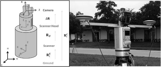
Sensor-side instrumentation is an approach to circumventing the need for artificial targets. Specifically, scanner-mounted GNSS antennas have been used to resolve position and angular orientation directly. These methods remove the necessity for external references altogether. The authors of [21] and [22] used up to two scanner-mounted GNSS antennas and an inclinometer to directly georeference the TLS data. The approach effectively resolved transformation parameters (per-profile heading and position) via an Extended Kalman Filter. The authors of [23] and [24] presented a method that uses two GNSS antennas mounted on the scanner to directly georeference lidar data by using the motion of the scanner head to derive the six transformation parameters. This paper is an extension of that research. It presents an augmentation of the previous method by incorporating close range photogrammetry enabled by a scanner-mounted camera, and test results of multiple “configurations” or combinations of sensor data and processing methods in terms of estimated uncertainty and check point-evaluated accuracy. A general model for georeferencing the TLS data through least-squares adjustment given the presented sensor configuration is provided.

2. Methods

This section describes the observations and mathematical model for a simultaneous least-squares adjustment of georeferencing parameters. Observations obtained from the dual antenna system, a scanner mounted camera, and the laser scanner itself are described in the following subsections.

2.1. The Dual-Antenna System

The dual antenna system (DAS) as presented in [23] and [24] consists of two scanner-mounted GNSS antennas as shown in Figure 1. The antennas are mounted on a stiff bar apparatus that is attached to and rotates with the scanner head about the z -axis of the scanner system. The essence of all DAS processing methods is that kinematic carrier phase methods are used to obtain vectors between the antennas, and absolute positioning using a nearby CORS as a base. When the head of the scanner is stationary the scanner coordinate system vector between antenna phase centers, Δ x S , is established from system calibration and rotation encoders in the scanner. The GNSS-observed vector is Δ x G . With a sufficient number of observations at diverse angular orientations of the scanner head, or “stops,” the relationship in Equation (2) can be used to solve for Euler angles associated with R S .
Δ x S = R S Δ x G .
The position component, t G , is found using the known position of the antennas with respect to the scanner system origin (leverarm). With a practical number of stops, the Euler angles can be resolved with a precision less than 1 mrad/σ. DAS methods can be divided into low-level, medium-level, and high-level integration with respect to how they included in a combined adjustment.

2.1.1. Low-Level DAS

Low-level DAS is the inclusion of all individually measured vectors for each GNSS epoch at each stop. This mode of integration is cumbersome due to the large number of observations produced and the need to model and include the correlation of errors between each epoch. It is thus not included in this study.

2.1.2. Medium-Level DAS

In medium-level DAS integration, there is no a priori solution. The weighted average of vectors, Δ x G , for each stop l at each station i serve as observations in subsequent adjustment and are contributed via Equation (2).

2.1.3. High-Level DAS

High-level DAS integration uses the a priori solution of Equation (2) for the georeferencing parameters, and includes the results as direct observations of the unknowns in a subsequent adjustment.
In general, the tilt components, rotation about the x and once-rotated y -axes ( ω and ϕ , respectively) are more weakly resolved than rotation about the twice-rotated z-axis ( κ ) due to the relative imprecision of the GNSS z component. This can be somewhat ameliorated by splitting the high-level DAS solution into two, one for tilt angles and one for κ . The tilt angles are resolved using the relationships shown in Equations (3)–(5).
R S Δ x G = Δ x S = [ r 11 r 12 r 13 r 21 r 22 r 23 r 31 r 23 r 33 ] [ Δ x Δ y Δ z ] G = [ Δ x Δ y Δ z ] S
[ r 31 r 23 r 33 ] [ Δ x Δ y Δ z ] G = Δ z S
Δ x G sin ϕ Δ y G sin ω cos ϕ + Δ z G cos ϕ cos ω Δ z S = 0.
Note in Equation (5) that the horizontal components in the scanner system Δ x S ,   Δ y S are not used, thus there is no need to observe the scanner head angle from which they are derived. This means that every GPS epoch can be used to develop an observation equation, and any errors in the encoder or horizontal leverarm do not contaminate the solution. Tests indicated that this method resulted in significantly more accurate tilt angles than by using solely using Equation (2). For further explanation and analysis of the DAS methods, please refer to [23] and [24].
Figure 1. The dual antenna system (DAS) mounted on a Riegl VZ400. Both the GNSS antennas and camera are fixed to the scanner head, which rotates during acquisition, and can rotate on-demand based on user input.
Remotesensing 07 11621 g001

2.2. Scanner Observations

2.2.1. Tie Points

Tie point observations consist of measured scanner-system coordinates, x i ,   j S , via artificial targets. They are introduced into the adjustment using Equation (1), where multiple x i ,   j S are associated with a single x   j G .

2.2.2. ICP

ICP contributions to the adjustment include observations of the relative angular orientation, Δ R i l , and translation,   Δ t i l , each from scanner system i   to scanner system l . The relationship between the observations and georeferencing parameters is shown in Equation (6).
R l S t l G Δ R i l R i S t i G Δ t i l = 0 ,

2.3. Image Observations

2.3.1. Camera Coordinate System

Image observations necessitate the definition of a camera coordinate system and its relationships to the scanner coordinate system. Figure 2 is a graphical depiction of these relationships. The rotation matrix from reference coordinates to the camera coordinate system is defined as: R i , θ C = Δ R R θ R i S . The matrix   R θ , shown in Figure 2, represents the angular orientation of the scanner head due to rotation about the scanner coordinate system z-axis by angle θ. Thus  Δ R , the boresight alignment also shown in Figure 2, is the rotation from the (rotated) scanner head system to the camera coordinate system. Similarly, the location of the camera perspective center in the reference coordinate system is t i , θ   C . The leverarm, Δ X = R i , θ C ( t i G t i , θ C ) , is the offset from the camera perspective center to the scanner-system origin in the camera coordinate system. Note that since the leveram is defined in terms of the camera system, it is independent from the rotation of the scanner head. This is assuming the rotation is about some vector passing through the scanner system origin (in our case the scanner system z axis).
Figure 2. Relationships among the camera, scanner and reference/ground coordinate systems. Each coordinate system is linked via the rotation matrices shown on the right-side of the figure.
Remotesensing 07 11621 g002

2.3.2. Collinearity Condition

Each imaged point (corrected for camera calibration parameters), k, measured at the i th setup in the camera coordinate system has the homogeneous form:
x i , k I =   ( x y f ) i , k I .
The collinearity condition is shown in homogeneous representation in Equation (7). Note, the scale factor, s , cancels when projecting from object space to image space.
x i , k I = s ( R i , θ C ( x k G t i G ) + Δ X ) .

2.3.3. Coplanarity Condition

The coplanarity condition may be used when object space coordinates of imaged points are not observed or to be resolved, and pair-wise image configuration is sufficient. In this case, the use of coplanarity over collinearity decreases the complexity of adjustment procedures since no a priori approximations of object space coordinates of points are necessary. The coplanarity condition equation for some pair of images i and l is shown in Equation (8). Note that in Equation (8) the angle θ associated with stations i and l may be different.
( t l , θ C t i , θ C ) · ( ( R i , θ C ) T x i , k I × ( R l , θ C ) T x l , k I ) = 0.

2.4. Solution

A simultaneous least-squares adjustment was used to solve for all transformation parameters via Equation (9), where: J is the Jacobian matrix containing partial derivatives of the observation equations with respect to the unknown transformation parameters; W is the weight matrix, the inverse of the full covariance matrix associated with the observations; k contains the measured minus computed values associated with observations; Δ contains corrections to the current-iteration approximations of the unknowns; superscript + indicates the pseudoinverse; and superscript 1 / 2 indicates the matrix square root. Note direct observations of unknowns were included via additional rows in J and diagonal blocks in W , similar to the method described for bundle adjustment solution in [25]. The eigen-decomposition matrix square root was used: M = Q Λ Q T M 1 / 2 = Q Λ 1 / 2 Q T . The singular value decomposition method of developing the pseudoinverse was used instead of the perhaps more-conventional method in order to mitigate ill-conditioning issues: M = U S V T M + = V Λ 1 U T .
Δ = ( W 1 / 2 J ) + W 1 / 2 k .
Estimated uncertainties of the resulting parameters were calculated via Equation (10) for the a posteriori parameter covariance matrix, where s 0 is the standard error of unit weight.
Σ ^ = s 0 2 ( J T W J ) 1 .

3. Experiments

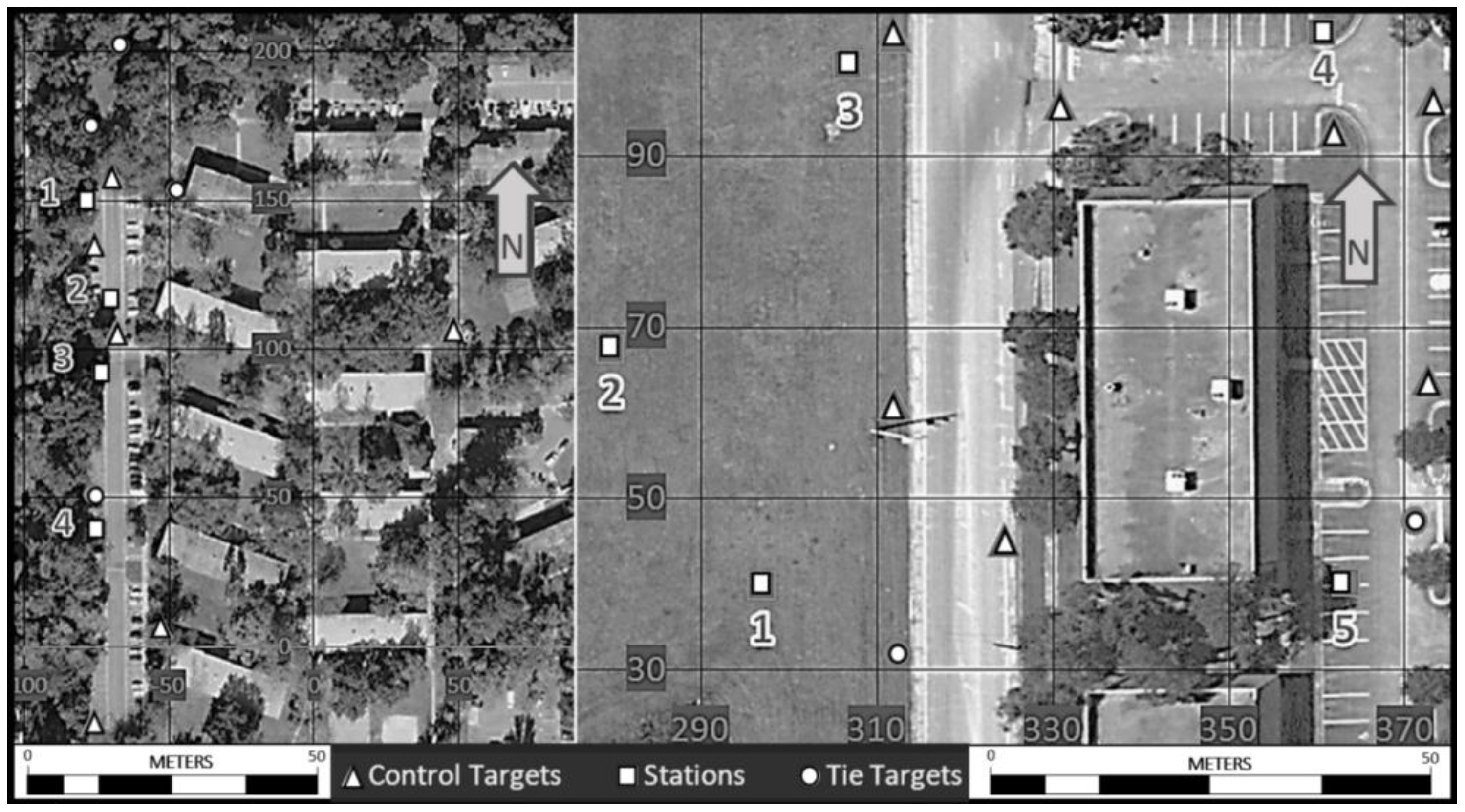
Two sites were chosen to compare various targetless adjustment configurations. The first was in Corry Village at the University of Florida campus in Gainesville, Florida (Site 1). The second was in Orlando, Florida near the Riegl USA offices (Site 2). The Site 1 data were characterized by poor geometry of scan stations target distribution. The Site 2 data had closer to optimal geometry with both stations and targets well-distributed throughout the site. Furthermore, Site 2 had fewer trees near scanner stations, and therefore satellite signals were less occluded. Figure 3 shows each site and associated scan stations and target locations. The Site 1 project had four stations and ten artificial targets, six of which had surveyed control coordinates. The Site 2 project had five stations and nine artificial targets, seven of which had surveyed control coordinates. Control coordinates were obtained using post-processed static GPS, and had estimated absolute horizontal and vertical uncertainties of about 1 cm/σ horizontal and < 2 cm/σ vertical for Site 1, and 1 cm/σ horizontal and < 1 cm/σ vertical for Site 2. 
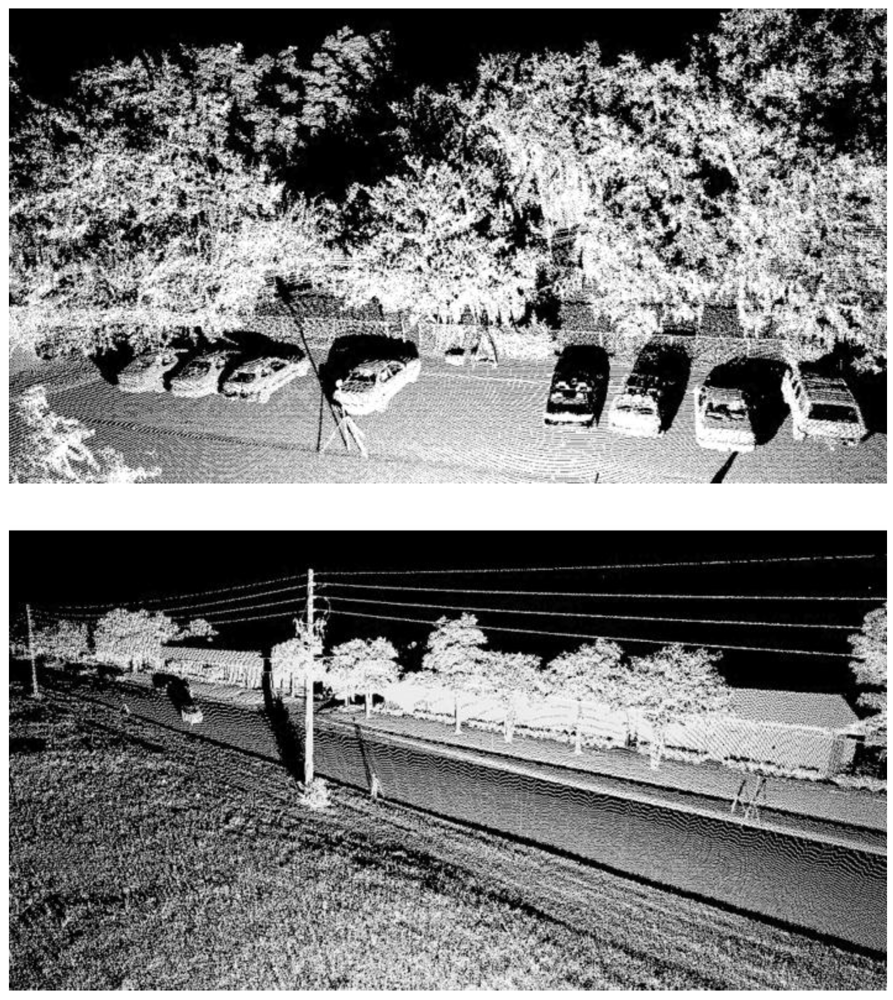
Figure 4 shows point clouds from both data acquisitions. Riegl cylindrical retroreflector targets with 10 cm height and 10 cm diameter were used at both sites, and were fine-scanned such that the target was covered with approximately 10,000 points for approximate location determination via the scanner software. Although some targets were located relatively close to the scanner, as illustrated in Figure 3, no substantial ill effects of this on positional accuracy were observed. DAS data was collected at each site with effective stops lasting 30–60 seconds at 15° increments of a full 360° rotation. ICP was implemented using a precursor to the variant described in [26].
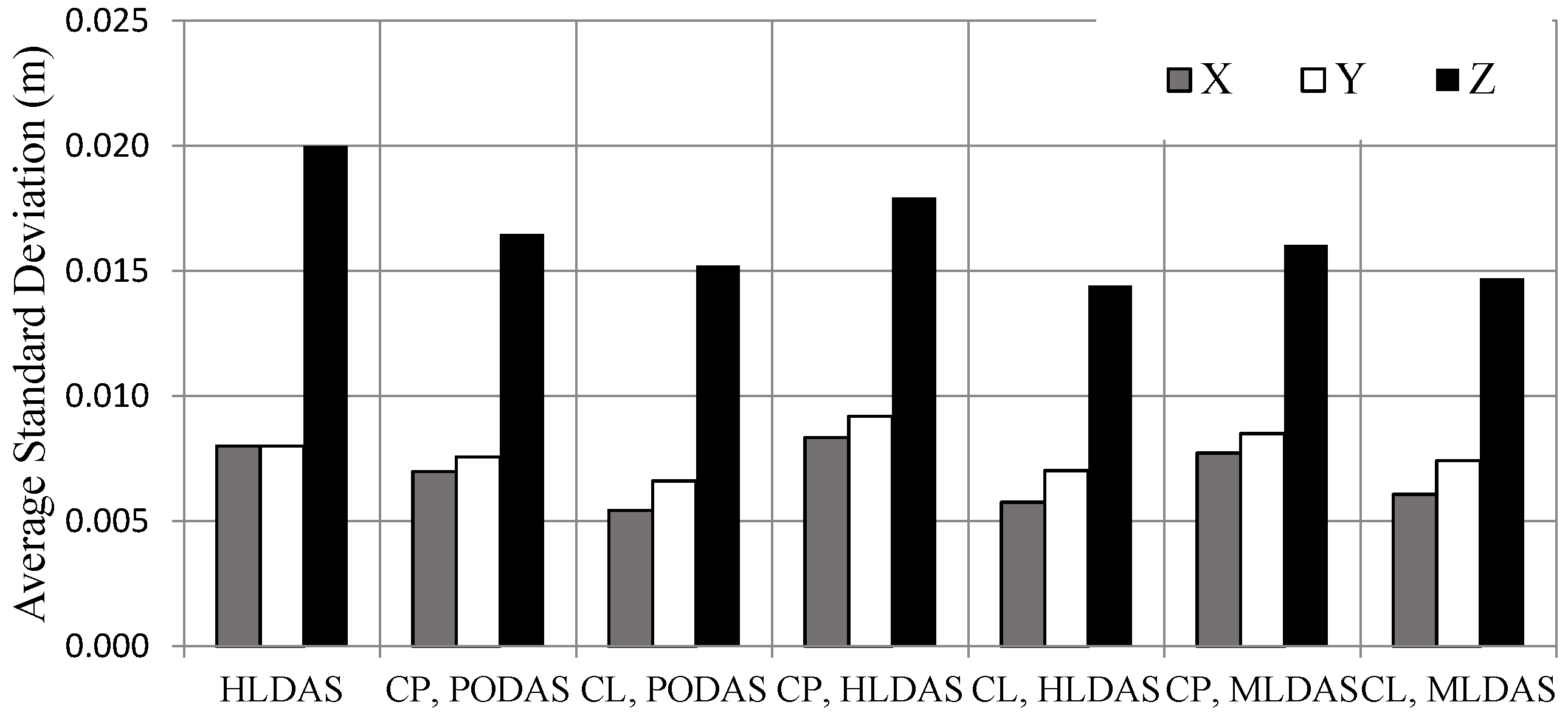
Multiple configurations, adjustments with different combinations of observations, were executed and the resulting estimated uncertainty and accuracy based on check points were recorded. The abbreviations in Table 1 are used to indicate which observations were used for each configuration. Nikon D300 and a Nikon D700 digital cameras fixed to the scanner were used at Site 1 and 2, respectively, to acquire imagery. Image observations included 308 individually measured image points (~1 pixel standard deviation) from 47 unique object space points in the Site 1 dataset, and 320 individually measured image points (~0.4 pixel standard deviation) from 73 unique object space points in the Site 2 dataset. Observations from ICP could only be made for three adjacent scans in the Site 2 dataset, due to presence of vegetation and occlusions illustrated in Figure 3 and Figure 4, exemplifying a fundamental problem with point cloud matching techniques in general.
Figure 3. Test locations at Site 1 in Corry Village (left) and Site 2 in Orlando (right). Site 1 is characterized by dense tree-cover and multiple buildings which constrained the distribution of targets. Site 2 allowed for a wider target distribution. Units of the arbitrary project coordinate system are in meters (Map data: © Google).
Remotesensing 07 11621 g003
Figure 4. Single-station point clouds at Site 1 from approximately the perspective of Station 3 looking northeast (top), and Site 2 from approximately the perspective of Station 1 looking northeast (bottom).
Remotesensing 07 11621 g004
Table 1. Observation Abbreviations.
AbbreviationObservationsDescription
CLCollinearityImage observations in the form of manually-mensurated conjugate points were included in the adjustment via the collinearity condition
CPCoplanarityImage observations in the form of manually-mensurated conjugate points were included in the adjustment via the coplanarity condition
PODASPosition Only DASOnly the position of the scanner derived from the DAS was used. This can be used to compare against more-conventional single-antenna systems, since the observations are similar (only position)
HLDASHigh Level DASHigh-level DAS observations were included
MLDASMedium Level DASMedium-level DAS observations were included
ICPIterative Closest PointIterative-closest-point observations were included
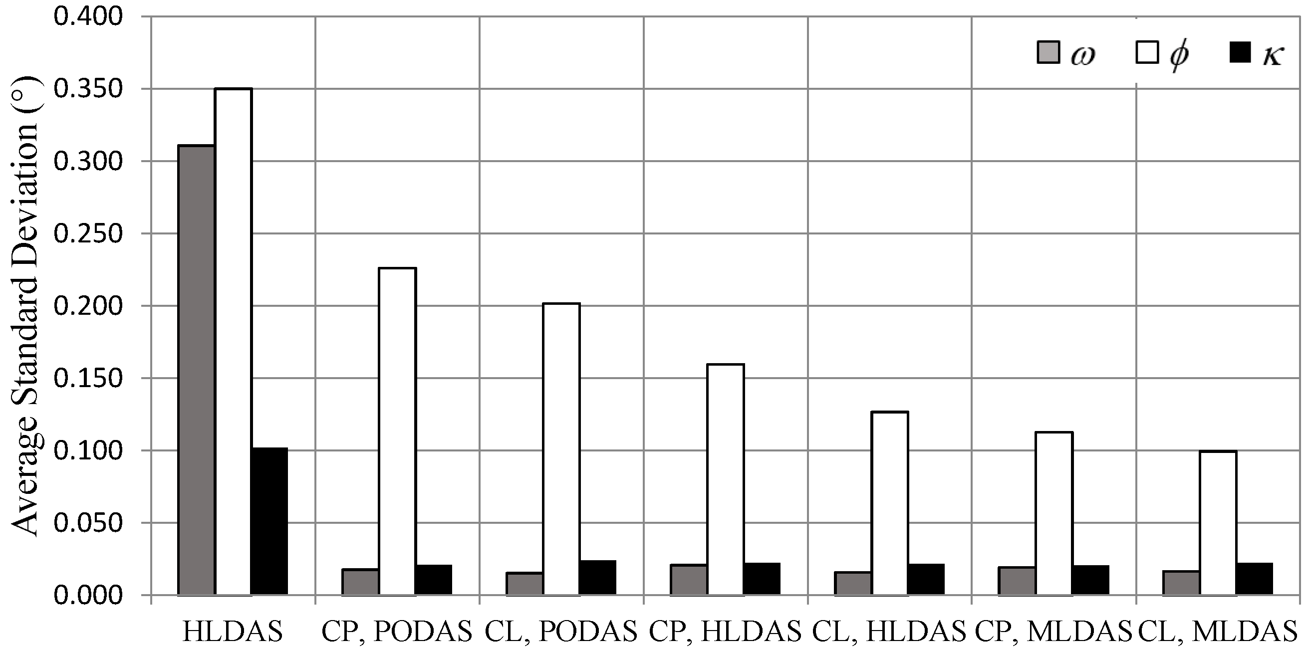
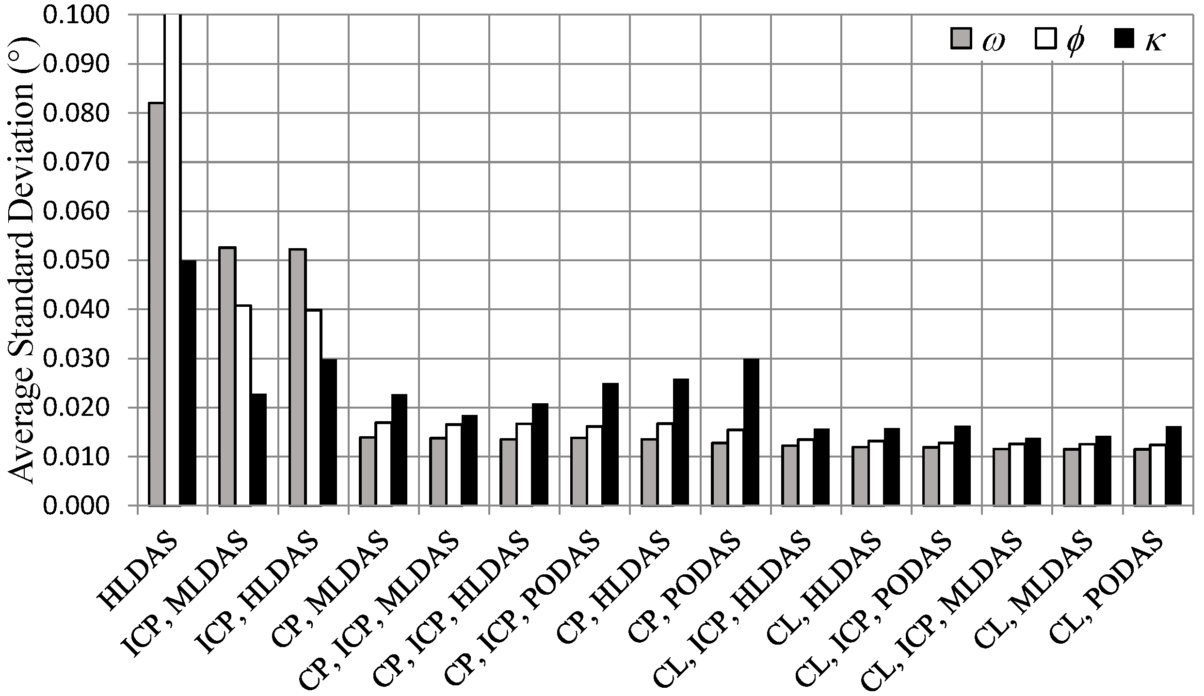
4. Results and Discussion

Results for estimated precision based on a posteriori standard deviations are shown in Figure 5, Figure 6, Figure 7 and Figure 8. RMSEs for each configuration are shown in Table 2 and Table 3. They are based on 18 check point coordinate sets for the Site 1 tests, and 24 for the Site 2 tests, where d h indicates horizontal RMSE. Only 14 checkpoints were used for ICP configurations that did not use image observations, due to not all stations being used. Estimated uncertainty for checkpoint targets were about 8.0 mm horizontal and 1.7 cm vertical ( 1   σ ) for the Site 1 data, where checkpoints had an average distance of 54 m from the scanner stations. The checkpoints used in the Site 2 data analysis had uncertainties of around 3 mm horizontal and 4 mm vertical ( 1   σ ) and were on average 40 m from the stations. Note that when only DAS observations are used (no image or scanner observations), MLDAS is the same as HLDAS, since they are both simply a direct solution of station transformation parameters. In this section, reported probabilities are based on F-tests of differences in variances. Analysis focuses on the most important results, although all configuration results are reported for completeness.

4.1. Site 1 Results

Table 2. Checkpoint RMSEs for Site 1.
MethodX (m)Y (m)Z (m)dh (m)
HLDAS0.0950.0211.4320.097
CP, PODAS0.0250.0060.0290.026
CL, PODAS0.0250.0060.0300.026
CP, HLDAS0.0200.0060.0230.021
CL, HLDAS0.0250.0050.0270.025
CP, MLDAS0.0200.0060.0240.021
CL, MLDAS0.0250.0050.0260.026
Figure 5. Average post-adjustment standard deviations for angular components of georeferencing parameters for the Site 1 dataset. Standard deviations were extracted from the a posteriori covariance matrix shown in Equation (10).
Remotesensing 07 11621 g005
Figure 6. Average post-adjustment standard deviations for positional components of georeferencing parameters for the Site 1 dataset. Standard deviations were extracted from the a posteriori covariance matrix shown in Equation (10).
Remotesensing 07 11621 g006

4.2. Site 2 Results

Inspection of Figure 5 shows that for Site 1, ϕ was generally the most weakly-resolved parameter due to the geometry of the project area. Image tie points were constrained to a north-south corridor due to occlusion by trees and buildings, which allowed substantial improvement of estimated ω and κ when using image points, but only a slight improvement in ϕ . The relatively low precision of ϕ is reflected in the Z component of the checkpoint RMSEs because error in tilt components is predominately propagated to the vertical component of point coordinates. This is also apparent in the DAS-only (HLDAS) case. Since the Δ z component of the DAS vectors is less precise than the horizontal components, ω and ϕ are more imprecisely resolved than κ as shown in Figure 5, leading to a large Z RMSE shown in Table 3. There was no significant difference in solutions for scanner positions, as illustrated in Figure 6.
In general, results for Site 2 were more accurate than those for Site 1. This was because of the stronger geometry and more accurate GPS observations since there were fewer occlusive trees in the area. Note that κ was the key parameter for differentiating Site 2 experiments, vs ϕ as in Site 1. Image observations substantially increased the precision of both ω and ϕ . This is also a byproduct of the well-distributed stations in Site 2 compared to Site 1. The RMSEs of check point coordinates ranged from 0.007 to 0.015 m, 0.005 to 0.019 m, and 0.011 to 0.146 m in X, Y and Z components, respectively. As with Site 1, the most accurate results came from configurations using image observations paired with MLDAS or HLDAS observations. This shows that the inclusion of photogrammetric observations can significantly increase the accuracy of the DAS solution when using multiple stations to capture a scene. When using images and including the DAS angular observations, either directly or indirectly, checkpoints points were calculated with significantly more accurate horizontal positions (p < 0.10) than when using position-only observations, PODAS. Note that the PODAS method contributes observations in a manner similar to conventional single-antenna systems: only the position of the scanner is observed, not the angular orientation. These results also agree with the estimated uncertainty of κ, which had smaller variances for HLDAS and MLDAS methods than for PODAS methods (p < 0.10). The same cannot be said, however, for Z RMSEs and the associated uncertainties of tilt components, for which there were no significant differences when using HLDAS and MLDAS methods versus using their PODAS counterparts. This is due to the weakness of tilt components, associated with the relatively inaccurate vertical components of GPS vector observations. The excellent precision of κ is noteworthy since modern systems with integrated digital compasses have a nominal azimuthal precision of only about 1° ( 1   σ ) , which can grow to as high as 6° due to environmental interference [27]. Even HLDAS without image observations resulted in much more precise resolution of κ with 1   σ values of 0.1° and 0.5° for Sites 1 and 2, respectively. It can also be observed in Table 3 that MLDAS solutions were more accurate than HLDAS solutions, indicating that deeper-integration via primitive observations led to better results. While the differences between the two are not always significant, it is recommended to use MLDAS since it does not significantly add to collection or computation time.
There were small, but mostly insignificant differences in the results when using coplanarity vs using collinearity as the model for image observations. As mentioned previously, coplanarity has the advantage that initial approximations for object space coordinates of imaged points are not needed, reducing the effort required to process the data. We also found that coplanarity, due to the significant reduction in unknown parameters, led to much faster adjustment computation times. For example, the (CL, PODAS) adjustment associated with Site 1 took about 5 s, whereas that for (CP, PODAS) took about 0.5 s. However, some instability of the adjustment was observed when using coplanarity, initially; we observed slight oscillation about the solution on convergence. This was remedied by using Levenburg-Marquardt Algorithm in a manner similar to that presented in [28], and although it tripled the solution time, coplanarity methods remained significantly faster than collinearity methods.
Figure 7. Average post-adjustment standard deviations for angular components of georeferencing parameters for the Site 2 dataset for configuration that do not use artificial targets. Note, σ ϕ = 0.18 ° for HLDAS is truncated. Standard deviations were extracted from the a posteriori covariance matrix shown in Equation (10).
Remotesensing 07 11621 g007
Figure 8. Average post-adjustment standard deviations for position components of georeferencing parameters for the Site 2 dataset for configurations that do not use artificial targets. Standard deviations were extracted from the a posteriori covariance matrix shown in Equation (10).
Remotesensing 07 11621 g008
Table 3. Checkpoint RMSEs for the Site 2 dataset.
MethodX (m)Y (m)Z (m)dh (m)
HLDAS0.0140.0090.1460.017
ICP, MLDAS0.0120.0090.0980.015
ICP, HLDAS0.0120.0090.0940.015
CP, MLDAS0.0070.0050.0150.009
CP, ICP, MLDAS0.0070.0050.0150.009
CP, ICP, HLDAS0.0100.0080.0160.013
CP, ICP, PODAS0.0170.0140.0180.022
CP, HLDAS0.0090.0080.0170.012
CP, PODAS0.0170.0190.0170.025
CL, ICP, HLDAS0.0120.0070.0130.014
CL, HLDAS0.0110.0060.0130.012
CL, ICP, PODAS0.0150.0090.0130.018
CL, ICP, MLDAS0.0100.0060.0110.011
CL, MLDAS0.0090.0050.0110.010
CL, PODAS0.0140.0080.0130.016
Effectively all presented methods of collection and processing are automatable. Although in this study image points were measured manually, it would be relatively simple to automate conjugation using one the many automatic algorithms available, such as that described in [19]. Similarly for the DAS collection routine, the method presented in Section 2.1.3 can potentially allow DAS observations to be collected during scanning, reducing the number of stops required.

5. Conclusions

Previous studies showed that using a dual GNSS antenna system (DAS) attached to a terrestrial laser scanner (TLS) can eliminate the need for artificial targets in georeferencing and registration since it provides both the position and angular orientation of the scanner directly. However these initial studies indicated that this was at the cost of accuracy especially in unfavorable GNSS conditions, provided only rudimentary methods for processing the data, and lacked guidance for simultaneous adjustment of scan data from multiple vantages. This paper extended that work by addressing these deficiencies. Specifically, new methods for rigorously registering and georeferencing TLS data using a DAS and photogrammetric data via a scanner-mounted camera were described, along with a model that accommodates these sensors that can serve as a general framework for error-propagation, uncertainty estimation, and adjustment of TLS data from similar systems.
Results from tests of multiple combinations of various techniques and observations were given, showing that including “lower-level” DAS observations (vectors between GNSS antennas as opposed to independently-determined angles) in comprehensive data adjustment results in higher accuracy, and that angular observations from the DAS significantly increased data accuracy compared to conventional single-antenna methods. Likewise, it was shown that the inclusion of photogrammetric observations in DAS-based adjustments can be used to effectively register and adjust data from multiple scan stations, and significantly improve TLS data accuracy. The inclusion of camera observations, which can easily be obtained from many contemporary TLS systems, in combination with DAS observations is a viable option for project areas where target placement is impeded and point cloud matching methods cannot be used due to lack of suitable features or complex scenes such as those that are highly-vegetated. These methods were shown to be feasible ways to reduce or eliminate the need for artificial targets in registering and georeferencing TLS data while maintaining useable accuracy.
Datasets from two study sites were used for testing. The first site was characterized by weak geometry of the scanner stations, which were constrained to being placed along a corridor, and poor GNSS signal reception. Using the DAS alone yielded horizontal and vertical accuracy of 0.10 m RMSE and 1.432 m RMSE for check points, respectively. Including photogrammetric observations in the adjustment significantly improved the accuracy, with best results of 0.021 m RMSE and 0.023 m RMSE for horizontal and vertical point coordinates, respectively. This showed that these observations can mitigate uncertainty, especially in tilt components of the scanner that manifest in the poor vertical accuracy of points.
The second site had much more favorable conditions and therefore stronger geometry, with scanner stations well-distributed around the project area. Results from using the DAS alone demonstrated higher accuracy than in the first site, with horizontal and vertical check-point RMSEs of 0.017 m and 0.146 m, respectively. Still, the inclusion of photogrammetric observations significantly increased the accuracy, with the best solution achieving 0.010 m RMSE and 0.011 m RMSE for the horizontal and vertical components, respectively. In one exemplary case, when using coplanarity-based photogrammetric observations, the solution that used only position (simulating a single-antenna system) yielded 0.025 m RMSE and 0.017 RMSE for the horizontal and vertical components, whereas when using the same photogrammetric observations and full DAS observations, the horizontal RMSE was 0.009, and the vertical RMSE was 0.015. As mentioned previously, low-level DAS solutions were generally more accurate than high-level solutions, and although the differences between the two are not always statistically significant, it is recommended to use low-level DAS.
Also explored was the method of including photogrammetric observations. The coplanarity model was found to be ten times faster in implementation than collinearity. However, using coplanarity sometimes led to solution instability. Although the instability was mitigated by using the Levenburg-Marquardt Algorithm, care should be taken when using this model for photogrammetric adjustment, especially in extreme geometric configurations.
Many of the observations in this work were obtained or processed manually. This includes the initial processing of the GNSS vectors associated with the DAS and the tie-point image observations, both of which take a significant amount of time. Since the overarching goal of this work is to provide accurate, direct, targetless methods for georeferencing TLS data automatically, future work will include investigating automatic methods for both the DAS processing steps and conjugate image point generation. There are many viable methods for automatic image matching. The starting point for automating the DAS processing was presented in this paper and involves separating the horizontal and vertical components of the GNSS vectors. It is envisioned that future iterations will allow for collection of DAS data during scan acquisition and automatic generation of DAS observations.

Acknowledgments

We acknowledge the kind contributions of Riegl USA for providing access to their laser scanners and expertise during the testing of the system.

Author Contributions

All authors contributed to the work presented in this paper. Ahmed Mohamed conceived the initial design and processing concepts for the dual antenna system, consulted on further refinement and analysis, and reviewed manuscript drafts. Benjamin Wilkinson developed the refined methods for the dual antenna system, developed the photogrammetric registration methods for multiple stations, implemented the processing algorithms, carried out the tests, analyzed the results, and wrote the manuscript. Bon Dewitt consulted on the refined algorithm designs and implementations, supported analysis of the results, and reviewed manuscript drafts.

Conflicts of Interest

The authors declare no conflict of interest.

References

  1. Vosselman, G.; Maas, H.S. Preface. In Airborne and Terrestrial Laser Scanning; CRC Press: Boca Raton, FL, USA, 2010; pp. ix–xii. [Google Scholar]
  2. Vosselman, G.; Maas, H.S. Registration and calibration. In Airborne and Terrestrial Laser Scanning; CRC Press: Boca Raton, FL, USA, 2010; pp. 83–133. [Google Scholar]
  3. Pesci, A.; Teza, G. Terrestrial laser scanner and retro-reflective targets: An experiment for anomalous effects investigation. Int. J. Remote Sens. 2008, 29, 5749–5765. [Google Scholar] [CrossRef]
  4. Mikhail, E.; Ackermann, F. Observations and Least Squares; IEP-A Dun-Donnelley Publisher: New York, NY, USA, 1976. [Google Scholar]
  5. Dewitt, B.A. Initial approximations for the three-dimensional conformal coordinate transformation. Photogramm. Eng. Remote Sens. 1996, 62, 79–84. [Google Scholar]
  6. Reshetyuk, Y. Self Calibration and Direct Georeferencing in Terrestrial Laser Scanning. Ph.D. Thesis, Royal Institute of Technology, Stockholm, Sweden, 2009. [Google Scholar]
  7. Silvia, E.; Olsen, M. To level or not to level: Laser scanner inclination sensor stability and application. J. Surv. Eng. 2012, 138, 117–125. [Google Scholar] [CrossRef]
  8. Rosser, N.J.; Petley, D.N.; Lim, M.; Dunning, S.A.; Allison, R.J. Terrestrial laser scanning for monitoring the process of hard rock coastal cliff erosion. Q. J. Eng. Geol. Hydroge. 2005, 38, 363–375. [Google Scholar] [CrossRef]
  9. Rowlands, K.A.; Jones, L.D.; Whitworth, M. Landslide laser scanning: A new look at an old problem. Q. J. Eng. Geol. Hydroge. 2003, 36, 155–157. [Google Scholar] [CrossRef]
  10. Royán, M.J.; Abellán, A.; Jaboyedoff, M.; Vilaplana, S.A.; Calvet, J. Spatio-temporal analysis of rockfall pre-failure deformation using Terrestrial LiDAR. Landslides 2013, 11, 697–709. [Google Scholar] [CrossRef]
  11. Hunter, G.; Pinkerton, H.; Airey, R.; Calvari, S. The application of a long-range laser scanner for monitoring volcanic activity on Mount Etna. J. Volcanol. Geoth. Res. 2003, 123, 203–210. [Google Scholar] [CrossRef]
  12. Olsen, M.; Johnstone, E.; Driscoll, N.; Ashford, S.; Kuester, F. Terrestrial laser scanning of extended cliff sections in dynamic environments: Parameter analysis. J. Surv. Eng. 2009, 135, 161–169. [Google Scholar] [CrossRef]
  13. Olsen, M.; Johnstone, E.; Kuester, F.; Driscoll, N.; Ashford, S. New automated point-cloud alignment for ground-based light detection and ranging data of long coastal sections. J. Surv. Eng. 2011, 137, 14–25. [Google Scholar] [CrossRef]
  14. Besl, P.J.; McKay, H.D. A method for registration of 3-D shapes. IEEE Trans. Pattern Anal. Mach. Intell. 1992, 14, 239–256. [Google Scholar] [CrossRef]
  15. Salvi, J.; Matabosch, C.; Fofi, D.; Forest, J. A review of recent range image registration methods with accuracy evaluation. Image Vis. Comput. 2007, 25, 578–596. [Google Scholar] [CrossRef]
  16. Al-Manasir, K.; Fraser, C.S. Registration of terrestrial laser scanner data using imagery. Photogramm. Rec. 2006, 21, 255–268. [Google Scholar] [CrossRef]
  17. Jansa, J.; Studnicka, N.; Forkert, G.; Haring, A.; Kager, H. Terrestrial laser scanning and photogrammetry—Acquisition techniques complementing one another. ISPRS Arch. 2004, 7, 948–953. [Google Scholar]
  18. Han, J.; Perng, N.; Chen, H. LiDAR point cloud registration by image detection technique. IEEE Geosci. Remote Sens. Lett. 2013, 10, 746–750. [Google Scholar] [CrossRef]
  19. Bay, H.; Ess, A.; Tuytelaars, T.; van Gool, L. Speeded-up robust features (SURF). Comput. Vis. Image Und. 2008, 110, 346–359. [Google Scholar] [CrossRef]
  20. Han, J.; Perng, N.; Lin, Y. Feature conjugation for intensity-coded LiDAR point clouds. J. Surv. Eng. 2013, 139, 135–142. [Google Scholar] [CrossRef]
  21. Paffenholz, J.A.; Kutterer, H. Direct Georeferencing of static terrestrial laser scans. In Proceedings of the FIG Working Week, Stockholm, Sweden, 14–19 June 2008.
  22. Paffenholz, J.A.; Bae, K.H. Geo-referencing point clouds with transformational and positional uncertainties. J. Appl. Geod. 2011, 6, 33–46. [Google Scholar] [CrossRef]
  23. Mohamed, A.; Wilkinson, B. Direct georeferencing of stationary LiDAR. Remote Sens. 2009, 1, 1321–1337. [Google Scholar] [CrossRef]
  24. Wilkinson, B.; Mohamed, A.; Dewitt, B.; Seedahmed, G. A novel approach to terrestrial LiDAR georeferencing. Photogramm. Eng. Remote Sens. 2010, 76, 683–690. [Google Scholar] [CrossRef]
  25. Wolf, P.R.; Dewitt, B.A.; Wilkinson, B.E. Elements of Photogrammetry (with Applications in GIS), 4th ed.; McGraw-Hill Education: New York, NY, USA, 2014. [Google Scholar]
  26. Bergström, P.; Edlund, O. Robust registration of point sets using iteratively reweighted least squares. Comput. Optim. Appl. 2014, 58, 543–561. [Google Scholar] [CrossRef]
  27. Böhm, J.; Haala, N. Efficient integration of aerial and terrestrial laser data for virtual city modeling using lasermaps. In Proceedings of the ISPRS Workshop Laser Scanning, Enschede, The Netherlands, 12–14 September 2005.
  28. Press, W.; Teukosky, S.; Vetterling, W.; Flannery, B. Numerical Recipes in C, 2nd ed.; Cambridge University Press: New York, NY, USA, 1992. [Google Scholar]

