Use of A Portable Camera for Proximal Soil Sensing with Hyperspectral Image Data

Abstract

In soil proximal sensing with visible and near-infrared spectroscopy, the currently available hyperspectral snapshot camera technique allows a rapid image data acquisition in a portable mode. This study describes how readings of a hyperspectral camera in the 450–950 nm region could be utilised for estimating soil parameters, which were soil organic carbon (OC), hot-water extractable-C, total nitrogen and clay content; readings were performed in the lab for raw samples without any crushing. As multivariate methods, we used PLSR with full spectra (FS) and also combined with two conceptually different methods of spectral variable selection (CARS, “competitive adaptive reweighted sampling” and IRIV, “iteratively retaining informative variables”). For the accuracy of obtained estimates, it was beneficial to use segmented images instead of image mean spectra, for which we applied a regular decomposing in sub-images all of the same size and k-means clustering. Based on FS-PLSR with image mean spectra, obtained estimates were not useful with RPD values less than 1.50 and R² values being 0.51 in the best case. With segmented images, improvements were marked for all soil properties; RPD reached values ≥ 1.68 and R² ≥ 0.66. For all image data and variables, IRIV-PLSR slightly outperformed CARS-PLSR.

1. Introduction

The demand for out-of-the-lab inventories initiated the early field spectroscopic experiments with non-imaging point measurements, which originated from laboratory spectroscopy and required respective developments in photonics and portable platform techniques, for example. From the beginning, portable or hand-held field spectroradiometers were very popular in soil spectroscopy [1,2,3] as they assured flexible and rapid data acquisition. Thus, spectroscopy in the visible (VIS) and near-infrared (NIR) has been widely used either in the laboratory [4,5,6,7] or for in-situ soil monitoring [8,9]. Non-imaging field spectroradiometers provide the highest available spectral resolution and thus high information content for estimating soil properties with multivariate methods. However, only integrative measurements can be performed, which hampers the analysis of spatial variability. Campaigns with portable field spectroscopy are often complemented by data of air- or spaceborne imaging spectrometers to cover larger areas; large area coverage in flight campaigns often leads to decreased accuracies of estimated soil properties compared to point measurements (due to a lower signal-to-noise ratio and disturbing atmospheric influences, for example). Variable soil and surface properties (as moisture content, roughness, crusting or texture) induce spectral variability that is critical for large-scale calibration approaches and may be met by stratified approaches [10,11,12].

In the described hyperspectral data chain, there is an obvious gap between integrative point measurements and airborne or even spaceborne image data, which may be filled by proximally sensed field hyperspectral image data. Field imaging line-scanners, however, are less widespread in ground truthing than portable point spectroradiometers, as operating a field line scanner on a tripod with a rotation stage is very time-consuming compared to the use of a point spectroradiometer. Non-scanning or snapshot hyperspectral imaging is one possible solution [13] to overcome this limitation and to bridge the gap in the data chain. It enables rapid data acquisition as the entire image with all spectra is captured at once within a few milliseconds in a hand-held or portable mode [14].

We could not identify other references in the field of proximal soil sensing with hand-held snapshot imaging spectroscopy. However, there is a rather broad list of studies conducted with line-scanners. Recently Steffens & Buddenbaum [15] used data of a hyperspectral scanner (spectral range 400–1000 nm) to determine the concentrations of carbon, nitrogen, aluminium, iron and manganese of a stagnic Luvisol profile under laboratory conditions; Stevens et al. [16], for example, provide an overview of available soil studies for air- and spaceborne scanning spectrometers. Furthermore, numerous studies exist that deal with ground-based scanning imaging spectroscopy (using the line-by-line approach on a rotation stage) for applications in geology, mineralogy and vegetation analysis [17,18,19].

Hyperspectral measurements always provide large sets of spectral variables that are strongly collinear and often noisy. The relationship between spectral values and soil constituents has to be modelled including data preprocessing and transformation. This can include a simple spectral index, with a combination of bands or based on absorption features [20], or the extraction of a number of factors or components after statistical data reprojection. These components should ideally represent the underlying information content of the data. After model calibration using wet-chemical reference values and validation (ideally external with an additional dataset, otherwise internal with e.g., leave-one-out cross-validation), this model may be applied to predict values for yet unknown samples.

In chemometrics, partial least squares regression (PLSR) has been firmly established as a robust multivariate calibration tool that is able to handle collinear and noisy data. Improvements in estimation accuracies are often achieved by selecting the most informative spectral variables instead of using the entire available spectral range. The optimal selection of spectral variables also tends to reduce the complexity of the multivariate model and the computational effort to finally retrieve estimates for the studied properties [21].

This paper focuses on the applicability of a non-scanning portable hyperspectral camera for soil sensing; all spectral readings used in this study were taken with the UHD 285 snapshot camera (Cubert GmbH, Ulm, Germany) that nominally covers the spectral range from 450–950 nm. A set of 40 soil samples taken from agricultural plots was spectrally measured in the laboratory to estimate the also wet-chemically determined contents of organic carbon (OC), nitrogen (N), hot water-extractable carbon (HWE-C) and clay (CL). These samples were previously used by Jung and Vohland [14] to compare image mean spectra with integrative (non-imaging) full range (400–2500 nm) spectroradiometer data and to analyse the effects of different states of crushing (raw, sieved and grinded) for chemometric modelling. Grinding and spectral variable selection was found to be necessary to obtain good results with the camera data, in which a fine crushing of course did not meet normal in-field conditions.

To overcome this limitation and to explore the applicability of the camera to field conditions, we only used raw samples in this study, i.e., soil samples were taken in-situ as grab samples from the topsoil, transported to the laboratory, only dried by airing and then carefully spread over an appropriate plate for spectral measurements. The aim was to analyse whether image segmentation (subdivision in square sub-images all of the same size and image portions defined by k-means clustering) and using the sub-image data instead of mean image spectra could enhance estimation accuracies. For multivariate modelling, we applied three strategies to all datasets: (1) Full spectrum (FS)-PLSR, (2) PLSR combined with a key wavelengths selection (CARS-PLSR) procedure [22] and (3) combined with the iteratively retaining informative variables (IRIV) selection method [23]. IRIV fundamentally differs from CARS as it considers joint effects of spectral variables. This paper is, as far as we know, the first contribution with a snapshot hyperspectral camera to proximal soil sensing (mimicking field conditions). As the successor of the UHD 285 is the UHD 185, an UAV enabled miniature hyperspectral camera with more than 100 spectral bands, we consider this study to be relevant for both proximal sensing in the field and mobile remote sensing using an autonomous platform.

2. Data Acquisition

2.1. Study Site, Sampling and Soil Wet-Chemical Analysis

The sampling area was located in Saxony in the natural region of the Saxon Loess Fields. Geologically, the sampled region was part of the Northwest Saxon Basin, which is characterised by Permian bedrock geology (rhyolites and ignimbrites), Cretaceous-Tertiary weathering products (like Kaolin) and quaternary sediments (loess, Pleistocene terrace gravel).

In the sampled region with a north to south distance of about 40 km, soil texture was markedly differentiated with sandy loess in the north and silty loess in the south. We randomly selected agricultural fields and took in total n = 40 samples from the very top layer (Ap, 0–10 cm depth). Soil texture therefore ranged from loamy sand (n = 2), sandy loam (11), loam (4), silt loam (22) to silt clay loam (1) (after FAO classification [24]); it was determined with the Köhn sieve-pipette method [25]. Contents of rock fragments or skeleton (>2 mm) were low in all cases (less than 10 percent by volume).

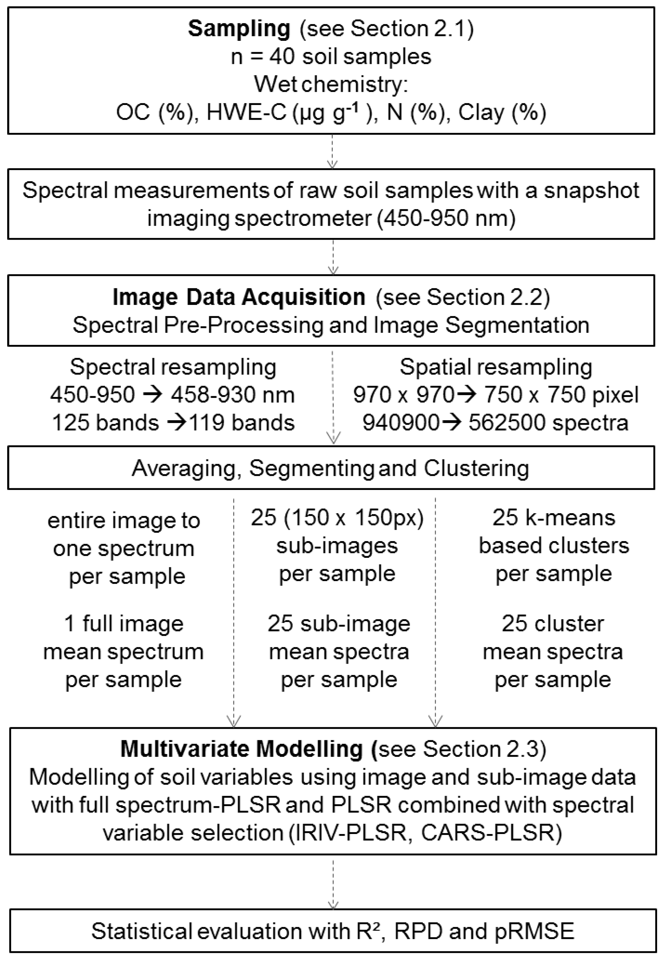
The workflow we followed after soil sampling is illustrated in Figure 1. Prior to wet-chemical analysis, soil samples were air-dried, sieved ≤ 2 mm, and subsequently homogenised by careful grinding using an agate mortar.

Figure 1. Workflow of the study.

Figure 1. Workflow of the study.

The total contents of OC and N were measured by dry combustion of samples at 1100 °C and gas chromatography using a EuroEA elemental analyser (HekaTech, Wegberg, Germany). All soil samples were free of carbonate-C. The HWE-C determination followed the method of [26] and was examined by a one hour extraction of 10 g soil with distilled water (50 mL) at 100 °C using a Gerhardt Turbotherm TT 125 (Gerhardt, Bonn, Germany). After the extraction, cooling, adding of MgSO₄ and centrifugation at 2600 rpm for 10 minutes, the dissolved organic carbon of the supernatant was analysed with a TOC-V_CPN-analyzer (Shimadzu, Duisburg, Germany). Table 1 illustrates mean, minimum, maximum, and standard deviation (stdv) of the analysed soil properties. In total, soil parameters given in Table 1 cover the typical values of agricultural soils.

Table 1. Wet-chemical parameters of the studied soil samples (n = 40).

Parameters	Mean	Min.	Max.	Stdv
OC (%)	1.54	0.62	4.31	0.74
HWE-C (μg·g−1)	652	306	1568	265
N (%)	0.145	0.048	0.377	0.068
Quotient C × N−1	10.9	8.5	18.0	2.2
Clay (%)	15.4	6.8	35.9	5.9

Table 1. Wet-chemical parameters of the studied soil samples (n = 40).

Parameters	Mean	Min.	Max.	Stdv
OC (%)	1.54	0.62	4.31	0.74
HWE-C (μg·g−1)	652	306	1568	265
N (%)	0.145	0.048	0.377	0.068
Quotient C × N−1	10.9	8.5	18.0	2.2
Clay (%)	15.4	6.8	35.9	5.9

2.2. Image Data Acquisition, Spectral Pre-Processing and Image Segmentation

All image data were captured with an UHD 285 hyperspectral snapshot camera. A hyperspectral non-scanning camera is generally designed to benefit from real-time data acquisition. A silicon CCD chip with a sensor resolution of 970 × 970 pixel captures the full frame images with a dynamic image resolution of 14 bit. In a normal sun light situation, the integration time of taking one hyperspectral data cube is 1 ms. The camera is able to capture more than 15 spectral data cubes per second, which facilitates hyperspectral video recording. The high-resolution imaging spectrometer coupled with the camera chip was designed and developed by ILM (Institute of Laser Technologies in Medicine and Metrology) at the University of Ulm and the Cubert GmbH, Germany. For our analysis, we used 125 spectral channels that cover the nominal spectral range from 450–950 nm. The hyperspectral data cube had a spectral resolution of 4 nm.

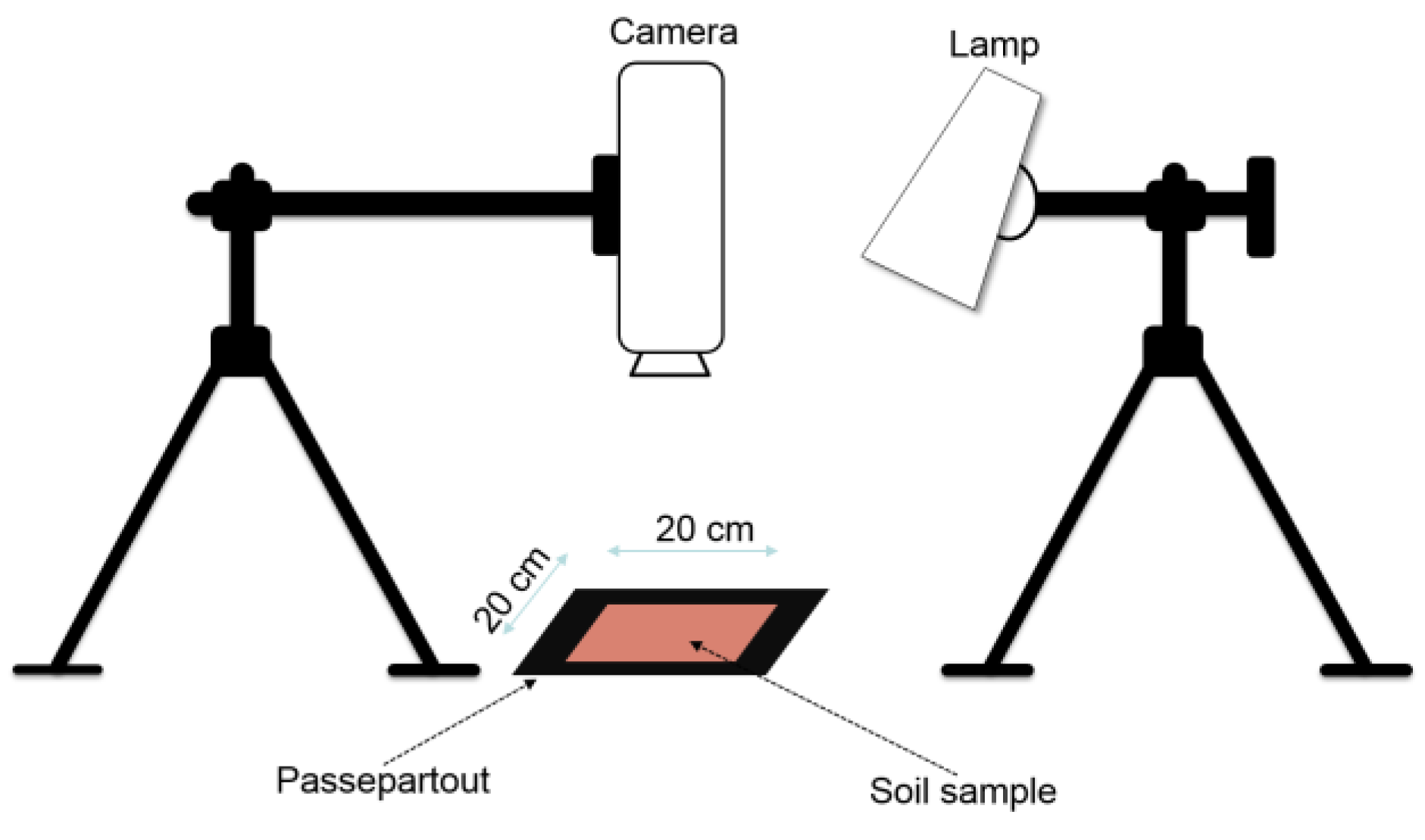
For the data collection, the camera was mounted on a single tripod (Figure 2). As an illumination source we used an ASD (Analytical Spectral Devices, Boulder, CO, USA) Pro-Lamp model (14.5 Volt, 50 Watt), which is also tripod-mountable for indoor laboratory diffuse reflectance measurements. The size of the calibrated reference panel (Zenith Polymer^®) was 30 cm × 30 cm.

The distance between sensor and soil sample was set to 35 cm in the nadir position, the illumination zenith angle was fixed at 45°. This illumination angle was selected as it is in line with prevailing midday illumination conditions e.g., in March or September in Central Europe, when soils are largely free of vegetation and allow for spectral inventories most easily. All raw samples were prepared on a reflection neutral plate (spectrally tested before) and covered, prior to the spectroscopic measurement, by a black passepartout (reflectance under 5% over the entire spectral range from 400–2500 nm) with a window of 20 cm × 20 cm. The native hyperspectral data cubes were converted into bsq (band sequential) format and processed in the following by the image analysis software ENVI (Exelis Visual Information Solutions, Boulder, CO, USA).

Figure 2. Experimental set-up with spectral snapshot camera and lamp in the laboratory.

Figure 2. Experimental set-up with spectral snapshot camera and lamp in the laboratory.

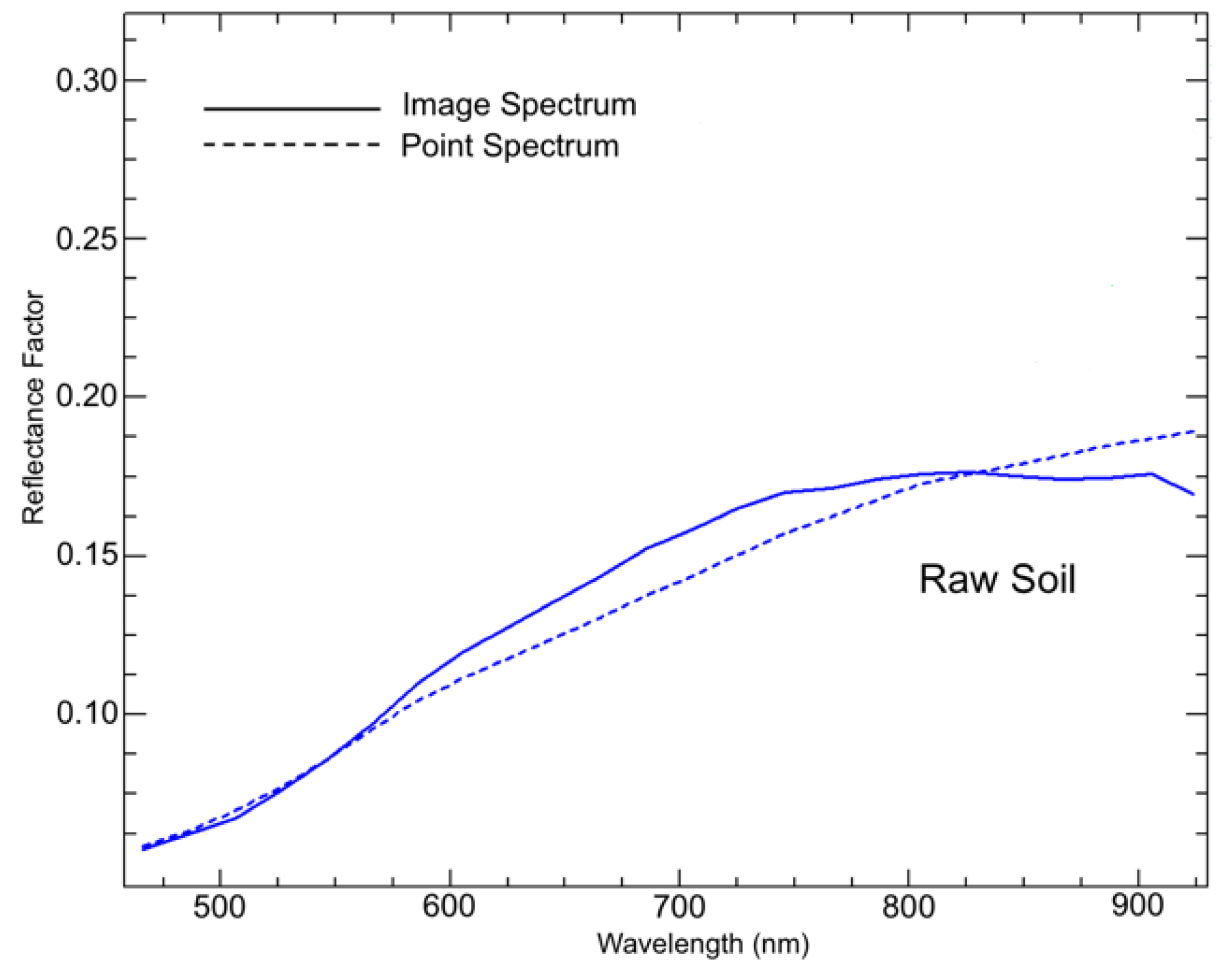
The measured spectra were reduced to 458–930 nm (119 spectral bands), as the first spectral bands below 458 nm showed non-correctable artefacts and the spectral region over 930 nm underwent a distinct Si-induced sensitivity loss. It is known for the silicon imaging technology that the light efficiency of the detector decreases from around 800 nm up to the response limit of the silicon detector [27], which to some extent can also be observed in the cut UHD spectra (Figure 3). Reflectance spectra were converted to absorbances with log (reflectance⁻¹). We also reduced the spatial dimension of the image data from 970 × 970 to 750 × 750 pixels as the near-border image portions often contained artefacts, which unreasonably changed the dynamic ranges of the image in all wavelengths.

Figure 3. Imaging and non-imaging reflectance curves (UHD camera vs. ASD spectroradiometer) measured for raw soil samples.

Figure 3. Imaging and non-imaging reflectance curves (UHD camera vs. ASD spectroradiometer) measured for raw soil samples.

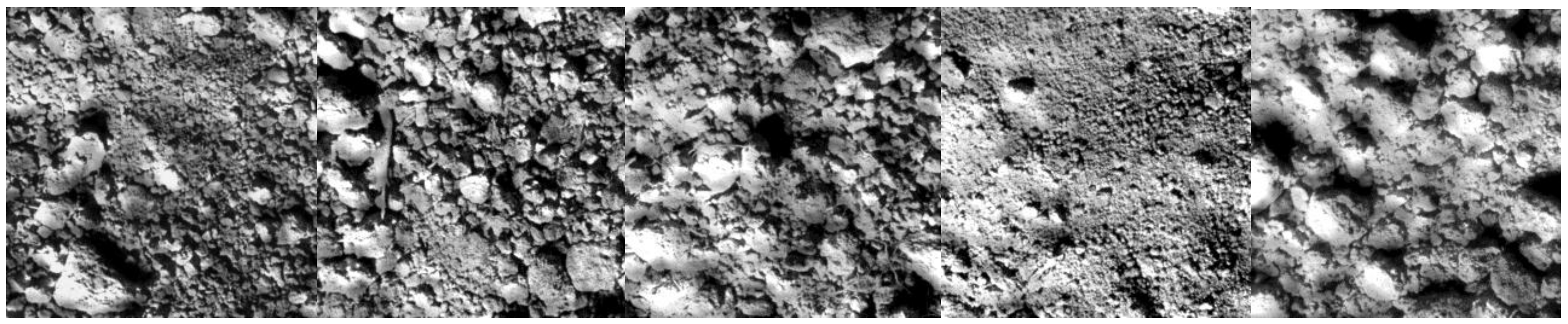
Figure 4. Examples of images (at 550 nm) for some selected soil samples with typical microstructures and illumination differences due to surface roughness (size of each image is 20 cm × 20 cm).

Figure 4. Examples of images (at 550 nm) for some selected soil samples with typical microstructures and illumination differences due to surface roughness (size of each image is 20 cm × 20 cm).

As an example, Figure 4 shows five soil sample images, which most appropriate characterizse our measurement situation in the laboratory. A number of effects influence the obtained measurements. Even for grinded samples, we have to be aware of effects due to different particle sizes [28]; reflectances general decrease with increasing particle size due to an increase of micro-shadows. Strong contrasts between illuminated and shadowed image regions result from the prevailing direct illumination of the light source (and a low diffuse illumination term). In addition, an irregular surface roughness induces a multidirectional (anisotropic) light scattering, which, for example, cannot be compensated by usual scatter corrections (as the standard normal variate [29] or the multiplicative scatter correction [30]).

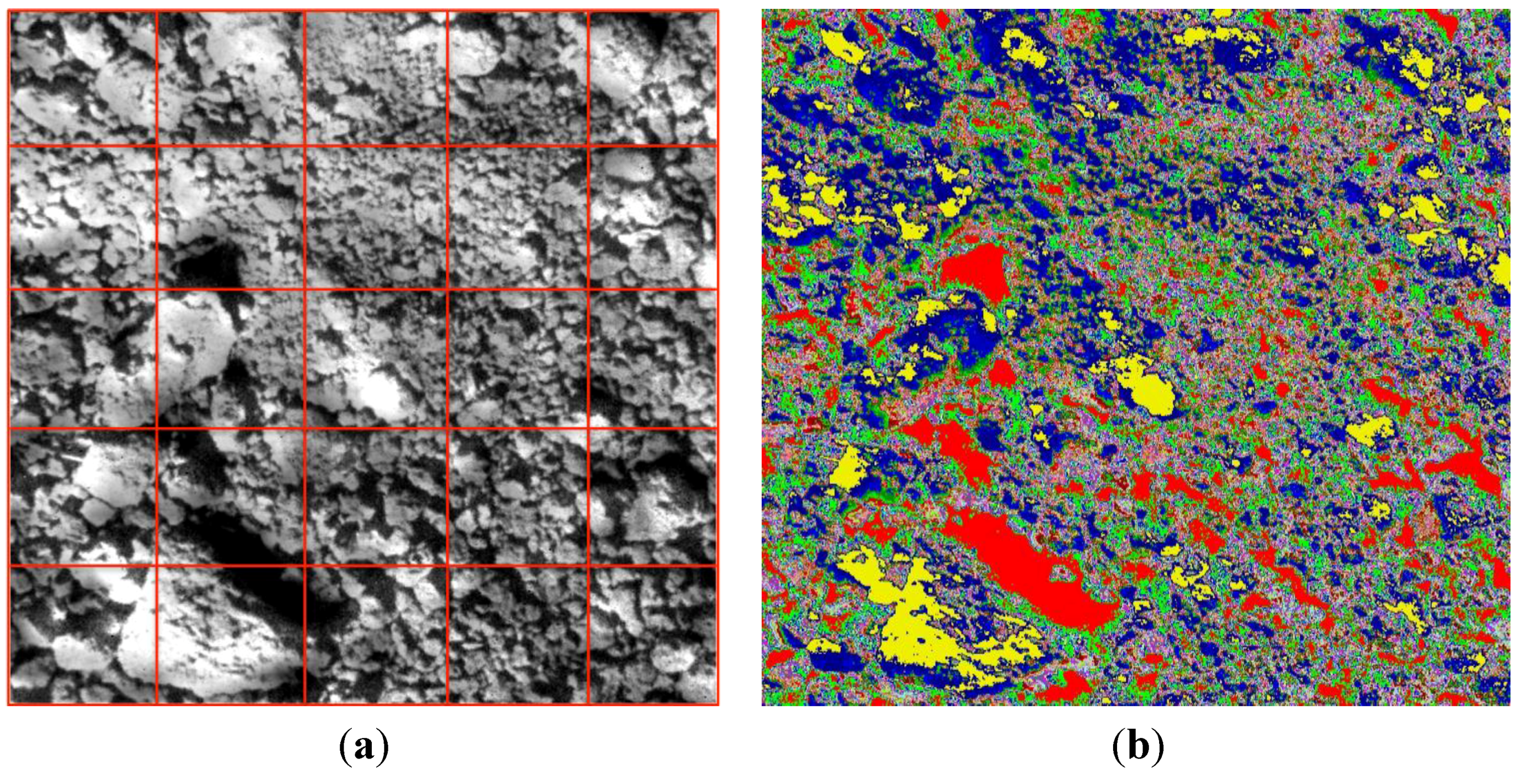
Image mean spectra (Figure 3), however, do not reflect the spatial and spectral variability within each image. To account for spatial variations of the spectral data, we used two approaches to divide the image spectral data cubes into 25 spatial sub-cubes or clusters. Grid-kind image segmentation divided the image into 25 regular sub-images (see Figure 5a); each sub-image represented 4% of the entire image (2500 pixels). In addition, we used a k-means clustering algorithm [31] applied in the spectral feature space with 119 channels to define 25 target clusters (Figure 5b).

Figure 5. Segmentation matrix (a) and k-means clusters (b) of a raw soil image.

Figure 5. Segmentation matrix (a) and k-means clusters (b) of a raw soil image.

2.3. Statistical Methods and Their Application to Obtain Estimates for Soil Variables from Image and Sub-Image Data

PLSR employs, similar to the more classical PCR (Principal Component Regression), statistical rotations to overcome the difficulties of high-dimensionality and multicollinearity. Unlike PCR, PLSR maximises the covariance between the spectral matrix (X) and the target chemical properties or soil constituents matrix (Y) to maximise the predictive capability of the resulting model [32]. To calibrate a PLSR model for each constituent, the number of latent variables was identified by performing a leave-one-out cross-validation (with the minimum root mean squared error RMSE as decision criterion), whereas a general limit was fixed at a maximum of 10. In addition to FS-PLSR, PLSR was also combined with CARS and the IRIV variable selection procedures.

The CARS selection procedure is based on the PLS regression coefficients of the individual spectral variables, whereas joint effects or interactions of the variables are not considered. For a detailed description of the CARS procedure, please refer to [22]. In brief, a series of sampling runs is performed with two successive steps of wavelengths selection to find an optimal subset (with the lowest RMSE in the cross-validation): First, an exponentially decreasing function removes all wavelengths with relatively small PLS regression coefficients. Second, an adaptive reweighted variable sampling is employed to additionally eliminate wavelengths in a competitive procedure. In this second refined selection step, random numbers are generated for variable selection, while the probability of each variable to be picked depends on its weight that is derived from the respective PLS regression coefficient. For our data set, a series of 50 successive sampling runs were performed. Due to the generation of random numbers in the second step, CARS-PLSR does not specify one unique “best” solution. Thus, we used CARS in an “ensemble mode”, i.e., the complete procedure was repeated 30 times and the final result for each sample was obtained by averaging all 30 estimates that generally were normally distributed.

IRIV considers the interaction of variables in the search space and performs a comparatively exhaustive search to keep only informative spectral variables. In addition to the spectral data matrix with n samples and p variables, a binary matrix with only 1 or 0 entries is generated. The binary matrix consists of k rows and p columns with k being defined as the number of random combinations of variables. For the PLSR modelling, each row of the binary matrix is considered while its entries determine which variables are to be used; in a five-fold cross validation, the performance of each subset is evaluated. In a next step, the models formerly defined are changed to derive each variable’s importance: Formerly included, a variable is now excluded (and vice versa) while the state of all other variables is kept unchanged. Modelling results obtained now are then compared to the former results. The statistical significance of found differences decide whether the variable is assumed to be strongly informative, weakly informative, uninformative or interfering. Only informative variables (both strongly and weakly) are kept; the entire procedure is repeated until no uninformative and interfering variables exist. Using backward elimination in the last step, the final list of informative variables is compiled [23]. Similar to CARS, no unique solution exists due to the randomness of combinations of variables contained in the binary matrix. We thus repeated the complete IRIV procedure as well 30 times and aggregated results by averaging.

In total, our dataset consisted of 40 images and 40 reference values for each constituent from the wet-chemical analyses (see Section 2.1). For the image mean spectra, we applied FS-PLSR, CARS-PLSR and IRIV-PLSR as described above and present the leave-one-out cross-validated results. For the sub-image analysis, we applied the already defined models (calibrated on the mean spectra) to all 25 subsets of each image, which resulted in 25 estimates per image. To exclude extreme values, we then only considered the values from the first to the third quartile and averaged them to obtain the final estimate for each image. In case of the clustered images, extracted values were additionally weighted using the respective image portions of the defined clusters.

We used the residual prediction deviation (RPD, defined as the ratio of the standard deviation of the reference values to the RMSE of the estimates), the relative RMSE (pRMSE = RMSE × measured arithmetic mean⁻¹) and the determination coefficient (R²) to assess the accuracy of the results.

3. Results and Discussion

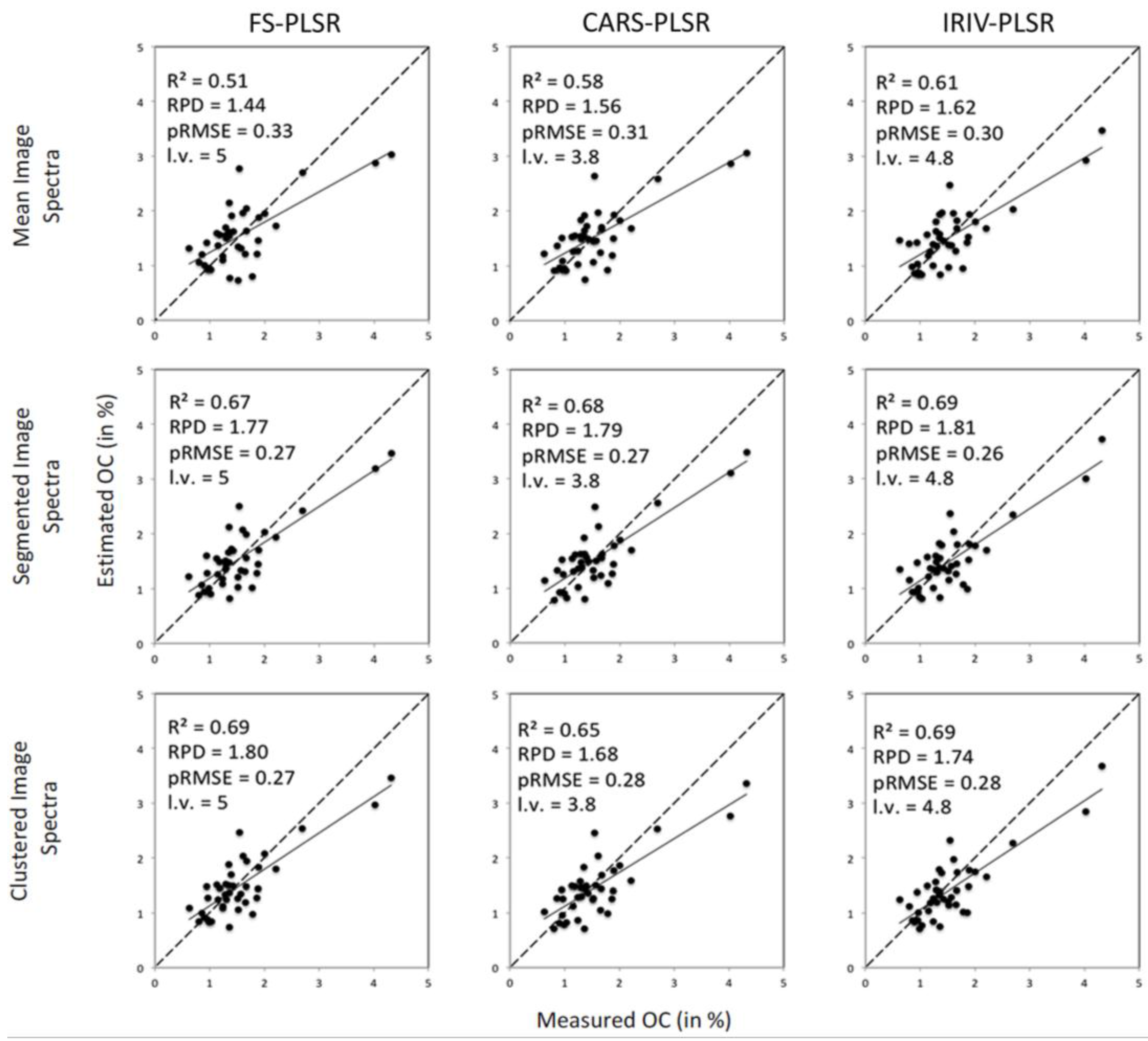
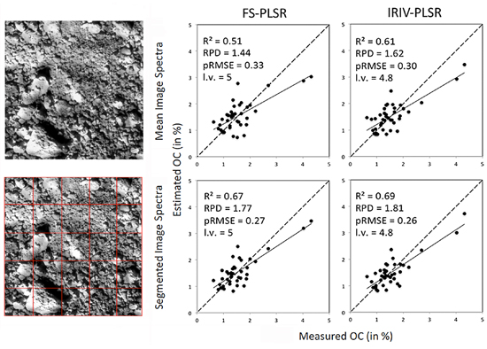
Estimates obtained with FS-PLSR, CARS-PLSR and IRIV-PLSR in the cross-validation (mean spectra) and from model application to segmented images are summarised for N, HWE-C and CL in Table 2; for OC, that is intrinsically coupled to soil organic matter and thus usually highly correlated with N (Pearsons’s r equalled 0.95 with p < 0.01) and HWE-C (0.93, p < 0.01), results are illustrated in Figure 6.

In case of averaged image spectra, we found for all constituents an order of obtained accuracies that was IRIV-PLSR > CARS-PLSR > FS-PLSR. Both variable selection methods outperformed FS-PLSR markedly, whereas IRIV-PLSR was slightly more successful than CARS-PLSR. This is in line with the original literature, as Yun et al. [23] also obtained better results with IRIV than with CARS, which was attributed to the IRIV strategy to consider the synergetic effects among the spectral variables. However, this strategy demands a runtime many times higher than that of CARS.

Table 2. Results from image spectra for raw soils (n = 40, best results for each image level and constituent in bold; l.v.: Number of latent variables; cv: Leave-one-out cross-validation; for segmented/clustered image data, models calibrated on image mean spectra were applied).

Image Level	Model	N				HWE-C				CLAY
		l.v. a	R2	RPD	pRMSE	l.v. a	R2	RPD	pRMSE	l.v. a	R2	RPD	pRMSE
Mean Image (MI) Spectra	FS-PLSRcv	5	0.48	1.40	0.05	6	0.48	1.38	191.6	5	0.49	1.41	4.17
	CARS-PLSRcv	3.7	0.59	1.59	0.044	3.0	0.54	1.49	178.4	4.2	0.65	1.72	3.42
	IRIV-PLSRcv	4.5	0.62	1.63	0.043	4.8	0.58	1.56	170.5	4.8	0.70	1.85	3.18
Segmented Image (SI) Spectra	FS-PLSR	5	0.63	1.65	0.042	5	0.62	1.64	162.1	5	0.64	1.44	4.09
	CARS-PLSR	3.7	0.63	1.66	0.042	3.0	0.58	1.55	171.3	4.2	0.66	1.50	3.92
	IRIV-PLSR	4.5	0.66	1.72	0.041	4.8	0.63	1.64	161.9	4.8	0.71	1.68	3.49
Clustered Image (CI) Spectra	FS-PLSR	5	0.65	1.65	0.042	6	0.70	1.85	145.1	5	0.71	1.51	3.88
	CARS-PLSR	3.7	0.63	1.62	0.043	3.0	0.58	1.55	170.7	4.2	0.70	1.39	4.22
	IRIV-PLSR	4.5	0.58	1.51	0.046	4.8	0.63	1.66	159.6	4.8	0.72	1.49	3.95

^a averaged from 30 runs for CARS-PLSR and IRIV-PLSR.

Table 2. Results from image spectra for raw soils (n = 40, best results for each image level and constituent in bold; l.v.: Number of latent variables; cv: Leave-one-out cross-validation; for segmented/clustered image data, models calibrated on image mean spectra were applied).

Image Level	Model	N				HWE-C				CLAY
		l.v. a	R2	RPD	pRMSE	l.v. a	R2	RPD	pRMSE	l.v. a	R2	RPD	pRMSE
Mean Image (MI) Spectra	FS-PLSRcv	5	0.48	1.40	0.05	6	0.48	1.38	191.6	5	0.49	1.41	4.17
	CARS-PLSRcv	3.7	0.59	1.59	0.044	3.0	0.54	1.49	178.4	4.2	0.65	1.72	3.42
	IRIV-PLSRcv	4.5	0.62	1.63	0.043	4.8	0.58	1.56	170.5	4.8	0.70	1.85	3.18
Segmented Image (SI) Spectra	FS-PLSR	5	0.63	1.65	0.042	5	0.62	1.64	162.1	5	0.64	1.44	4.09
	CARS-PLSR	3.7	0.63	1.66	0.042	3.0	0.58	1.55	171.3	4.2	0.66	1.50	3.92
	IRIV-PLSR	4.5	0.66	1.72	0.041	4.8	0.63	1.64	161.9	4.8	0.71	1.68	3.49
Clustered Image (CI) Spectra	FS-PLSR	5	0.65	1.65	0.042	6	0.70	1.85	145.1	5	0.71	1.51	3.88
	CARS-PLSR	3.7	0.63	1.62	0.043	3.0	0.58	1.55	170.7	4.2	0.70	1.39	4.22
	IRIV-PLSR	4.5	0.58	1.51	0.046	4.8	0.63	1.66	159.6	4.8	0.72	1.49	3.95

^a averaged from 30 runs for CARS-PLSR and IRIV-PLSR.

Figure 6. Estimated vs. measured values of OC (in %) obtained for image mean spectra and segmented images with three different PLSR approaches.

Figure 6. Estimated vs. measured values of OC (in %) obtained for image mean spectra and segmented images with three different PLSR approaches.

Wavelengths that were found to be important for the quantification of the studied soil properties are reported in Table 3. For both CARS and IRIV, selection frequencies obtained in all 30 runs were summed to total selection frequencies, and each spectral variable with a frequency adding more than 5% to total frequencies was categorized as a key wavelength. For OC and N, relevant wavelengths were found in the VIS and in the NIR range, but were missing in the red edge domain. For clay, both selection methods identified key wavelengths without any overlap to those of N and OC, which indicates the specificity of the spectral signature directly related to clay. The high correlation between HWE-C and OC suggests that a spectral quantification of HWE-C may be triggered by OC. However, identified key wavelengths show similarities in the VIS range, but deviations in the red edge and NIR domain, which may indicate a specific spectral basis for assessing HWE-C.

Table 3. Key variables selected by CARS and IRIV from the studied image spectra with 119 spectral variables (458–930 nm, 4 nm increment).

	CARS-PLSR				IRIV-PLSR
	Selections a	VIS (458–678 nm)	Red Edge (682–736 nm)	NIR (742–930 nm)	Selections a	VIS (458–678 nm)	Red Edge (682–736 nm)	NIR (742–930 nm)
OC	n = 367 sel; key wvl > 18 sel	no key wvl, but minor peaks at 470, 574, 666 nm	-	no key wvl, but minor peaks at 794, 834 nm	n = 350 sel; key wvl > 17 sel	562 570 574	-	854–866 902–910
N	n = 185 sel; key wvl > 9 sel	666	-	862	n = 210 sel; key wvl > 10 sel	610	-	862–866 906–910
HWE-C	n = 135 sel; key wvl > 6 sel	670–674	682	-	n = 408 sel; key wvl > 20 sel	574–578 610 678	718–722	-
CLAY	n = 260 sel; key wvl > 12 sel	482562	686	-	n = 279 sel; key wvl > 13 sel	428 490 510 522	690	834

^a sel=selections; n = number of total selections in all 30 runs; key wvl = key wavelengths.

Table 3. Key variables selected by CARS and IRIV from the studied image spectra with 119 spectral variables (458–930 nm, 4 nm increment).

	CARS-PLSR				IRIV-PLSR
	Selections a	VIS (458–678 nm)	Red Edge (682–736 nm)	NIR (742–930 nm)	Selections a	VIS (458–678 nm)	Red Edge (682–736 nm)	NIR (742–930 nm)
OC	n = 367 sel; key wvl > 18 sel	no key wvl, but minor peaks at 470, 574, 666 nm	-	no key wvl, but minor peaks at 794, 834 nm	n = 350 sel; key wvl > 17 sel	562 570 574	-	854–866 902–910
N	n = 185 sel; key wvl > 9 sel	666	-	862	n = 210 sel; key wvl > 10 sel	610	-	862–866 906–910
HWE-C	n = 135 sel; key wvl > 6 sel	670–674	682	-	n = 408 sel; key wvl > 20 sel	574–578 610 678	718–722	-
CLAY	n = 260 sel; key wvl > 12 sel	482562	686	-	n = 279 sel; key wvl > 13 sel	428 490 510 522	690	834

^a sel=selections; n = number of total selections in all 30 runs; key wvl = key wavelengths.

The specific effects of image segmentation can be demonstrated with FS-PLSR. Accuracy of estimates improved markedly when one of the segmentation approaches was applied. R² values improved at least to 0.62 (HWE-C with spectra from square sub-images), whereas without segmentation a maximum of 0.51 (OC) had been reached. With the exception of CL, RPD values were now at least 1.64 (compared to 1.30 before) (Figure 6, Table 2).

With image segmentation, the positive effects of spectral variable selection towards FS-PLSR were not as marked as with image mean spectra. For square sub-images, at least slight improvements were obtained for all soil properties with IRIV-PLSR. In total, best results were achieved with IRIV-PLSR on regularly segmented images for OC, N and CL; for HWE-C, FS-PLSR on clustered images was most successful (Figure 6, Table 2).

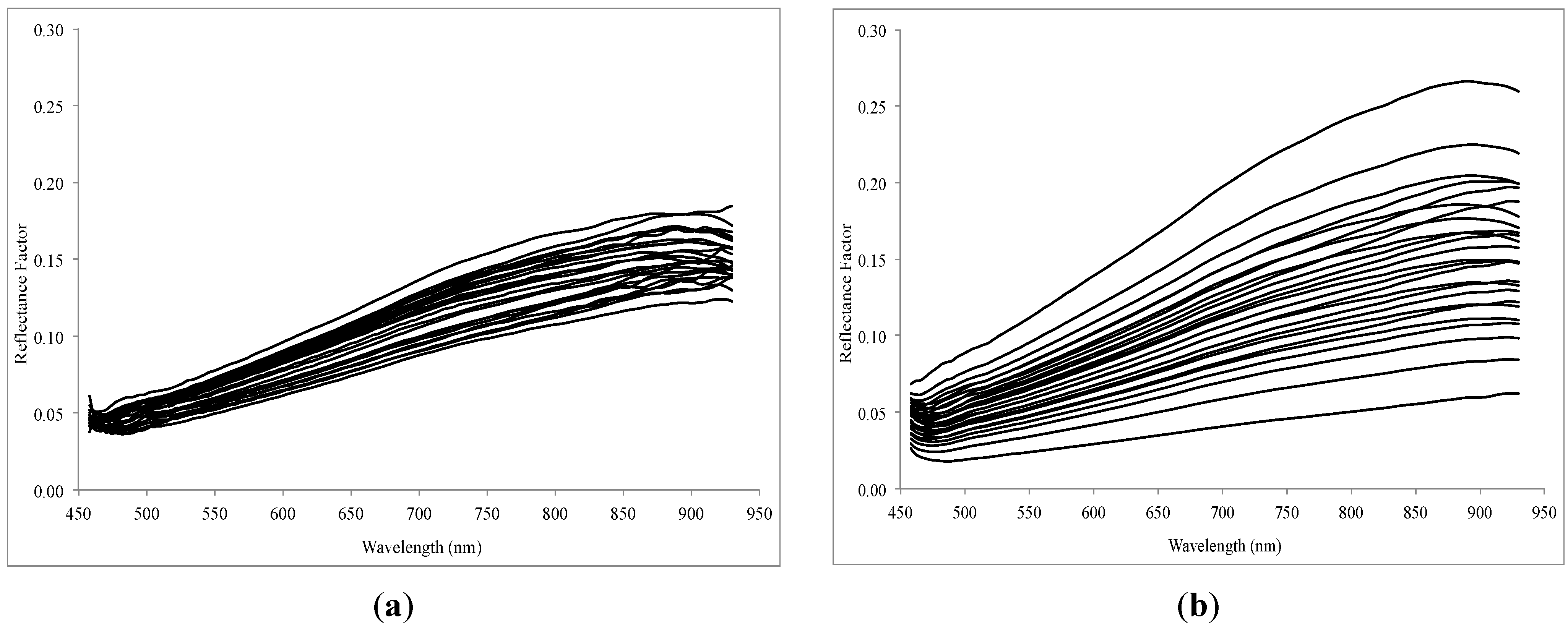
Especially for OC and N, we found accuracies dropping slightly when clustered images were used instead of regularly decomposed images (with CARS-PLSR and IRIV-PLSR). To analyse this finding we studied spectra of the sub-images for each case (Figure 7). In the case of regularly subdivided images, each sub-image contained (at least to a far degree) the micro-topography that was also typical for the entire image, i.e., shadowed areas as well as moderately illuminated parts or even hot spots. Thus, as the spectral information is averaged for each sub-image, we found an overall restricted variation of the spectra from one sub-image to another (Figure 7). With clustering—e.g., deepest shadows or hot spot areas are each attributed to one specific cluster—clusters represent, in addition to possibly different ranges of spectrally relevant soil properties, different illumination conditions and thus show a very pronounced spectral variability (Figure 7).

We have to be aware that our estimation procedure for segmented image data was based on PLSR models that had been calibrated on image mean spectra. Thus, in case of clustered data, a marked extrapolation was necessary which typically suffers from high insecurities and creates inaccuracy in estimates.

Figure 7. (a) Mean spectra of the 25 regular sub-images (Figure 5a) and (b) mean spectra of the 25 k-means clusters (Figure 5b).

Figure 7. (a) Mean spectra of the 25 regular sub-images (Figure 5a) and (b) mean spectra of the 25 k-means clusters (Figure 5b).

Our analysis indicated that in the images (although limited in size) there was a great variability of the contained (spectral) information. These fine-scale variations are relevant for chemometric approaches, as they require an appropriate definition of calibration sets that have to cover these variations adequately.

For the evaluation of the results, we have to consider the limited spectral range of the applied hyperspectral camera. In the SWIR domain (from 1000–2500 nm), a number of wavelength regions (e.g., the hydroxyl band at 2200 nm or wavelengths near the prominent water absorption band) have been shown to be essential for assessing OC [33,34,35,36]. Bellon-Maurel and McBratney [36] quote in their review paper the 1600–2500 nm range to be the most relevant for measuring OC, Cécillon et al. [37] present a compilation of important NIR wavelengths for OC and also N that were all beyond 1100 nm, and Lagacherie et al. [38] show the importance of the hydroxyl band for assessing clay.

Although the tested hyperspectral camera (UHD 285) did not cover the SWIR region, obtained values indicated, according to the guidelines of [39], approximate quantitative predictions (shown by R² values from 0.66–0.81) or at least the possibility to distinguish between high and low values (with RPD values between 1.5 and 2.0). With the same technology, measurements were also taken by another group [40], who applied the hyperspectral snapshot camera on an UAV platform for studies of vegetation and precision agriculture and emphasized the advantage of mobile mapping for field measurements. For field applications, both soil and vegetation spectroscopy will benefit from a non-scanning camera system covering the full spectral range from 400–2500 nm, which is a current technological challenge. For this future development, we assume our proposed approaches (variable selection, image segmentation) to be also of value for the retrieval of accurate estimates for soil properties. Our results were restricted to raw soil samples, which represent the normal in-field situation with rough soil surfaces. Soil surface roughness is known as one main disturbing factor for in-situ soil spectroscopy [41]. For larger sample sets, image data of the UHD have the potential to assess soil roughness classes directly from the images (e.g., by analysing the extent of shadowed image portions [42]) and thus to allow the implementation of stratified approaches for different soil roughness classes.

4. Conclusions

Our paper analysed the capability of a non-scanning hyperspectral imaging sensor with a nominal spectral range from 450–950 nm to provide data for the multivariate calibration of soil properties; we made a comparative analysis with three different PLSR approaches applied together with three image treatment methods. Analysed soil samples were not crushed to mimic a situation similar to in-field conditions.

It was shown that the simple use of image mean spectra for chemometric modelling did not exploit the potential of spatially distributed information contained in each image and resulted in poor estimates. Image segmentation distinctly improved the database for chemometric modelling and thus led to markedly improved estimates for the studied soil properties. This applied to both segmentation methods that were tested. Spectral variable selection was shown to enable further improvements concerning the accuracy of retrieved estimates. IRIV outperformed CARS, but it could become ineffective (due to very long runtimes) with larger datasets and a higher number of available spectral bands.

Nevertheless, care has to be taken, as documented for the analysed image spectra, for the completeness of the calibration set (which has to cover the full range of existing situations), as otherwise extrapolation to new situations will result in inaccuracies. Soil roughness influenced the performed spectral measurements considerably due to multidirectional scattering effects. This suggests another application of the camera data, which is to classify soil roughness—for example, based on shadowed image portions—and then to perform a stratified calibration on the hyperspectral datasets with different soil roughness strata.