Technical Note

Semi-Global Filtering of Airborne LiDAR Data for Fast Extraction of Digital Terrain Models

1
School of Remote Sensing and Information Engineering, 129 Luoyu Road, Wuhan University, Wuhan 430079, China
2
Collaborative Innovation Center of Geospatial Technology, Wuhan University, Wuhan 430079, China
3
Lyles School of Civil Engineering, Purdue University, West Lafayette, IN 47907, USA
*
Author to whom correspondence should be addressed.
Remote Sens. 2015, 7(8), 10996-11015; https://doi.org/10.3390/rs70810996
Submission received: 8 May 2015 / Revised: 24 July 2015 / Accepted: 20 August 2015 / Published: 24 August 2015
(This article belongs to the Special Issue Lidar/Laser Scanning in Urban Environments)

Abstract

:
Automatic extraction of ground points, called filtering, is an essential step in producing Digital Terrain Models from airborne LiDAR data. Scene complexity and computational performance are two major problems that should be addressed in filtering, especially when processing large point cloud data with diverse scenes. This paper proposes a fast and intelligent algorithm called Semi-Global Filtering (SGF). The SGF models the filtering as a labeling problem in which the labels correspond to possible height levels. A novel energy function balanced by adaptive ground saliency is employed to adapt to steep slopes, discontinuous terrains, and complex objects. Semi-global optimization is used to determine labels that minimize the energy. These labels form an optimal classification surface based on which the points are classified as either ground or non-ground. The experimental results show that the SGF algorithm is very efficient and able to produce high classification accuracy. Given that the major procedure of semi-global optimization using dynamic programming is conducted independently along eight directions, SGF can also be paralleled and sped up via Graphic Processing Unit computing, which runs at a speed of approximately 3 million points per second.

Graphical Abstract

1. Introduction

Since the 1990s, airborne Light Detection and Ranging (LiDAR) has been an important technological innovation in remote sensing and mapping science. LiDAR is capable of directly acquiring high-accuracy 3D coordinates of discrete points on the earth’s surface. The extraction of Digital Terrain Models (DTM) from airborne LiDAR point cloud has been an attractive research topic [1]. As both ground and non-ground objects (e.g. buildings, vegetation, and vehicles) reflect laser light, the first step towards generating a DTM from a LiDAR point cloud is classifying the point cloud into ground and non-ground points. This task is referred to as filtering. With the variations in scene complexity, LiDAR data filtering can be a difficult task, and its quality control procedure may consume approximately 60% to 80% of the total processing time [2,3]. Moreover, filtering is challenging for real-time applications or large-volume data processing.
Many techniques for separating ground and non-ground points from airborne LiDAR have been developed. The typical algorithms of filtering can be roughly categorized as follows: slope-based [4,5,6,7], linear prediction-based [8,9,10], mathematical morphology-based [11,12,13], progressive Triangulated Irregular Network (TIN)-based [14,15,16], and segmentation-based [17,18,19]. The merits and drawbacks of these methods have been reported [3,11,13,20]. The methods that estimate the properties of a local surface have been proven better than those that only detect elevation discontinuities [2]. This case implies that using the context of a wider range of points benefits filtering because such a context can employ more information to improve the classification accuracy. How to integrate different information into a certain extent of the point cloud plays an important role in the algorithm design. From this perspective, some algorithms (linear prediction [8,9,10]) use the local extent of the point cloud. This group of methods defines a local discriminant function based on which points are classified as ground and non-ground by the parameters or thresholds calculated from the neighboring points. The key to such algorithms is extracting ground or non-ground features from a group of neighboring points. Such an extraction is generally based on the assumption that the slope between a ground point and its neighboring ground point is gradual rather than abrupt. Generally, these algorithms perform effectively on flat terrains. However, discontinuities often happen on steep terrains, such as terraced fields, scarps, and steep forested areas [3]. Therefore, ground with discontinuities may be filtered out, which may cause a decline in accuracy [1]. To address such problems, global-based methods have been developed. Thin plate spline [1] and active shape model [21] model the ground point extraction from airborne LiDAR as a global optimization problem. The authors of [22,23] use the Markov Random Field (MRF) to label each point with different classes. On the one hand, global-based methods can use both the local and global features extracted from a larger extent of a point cloud. Experiments have shown that these methods can extract the smooth bare ground while preserving the discontinuities of steep terrains. In fact, the accuracy of the best known algorithms sometimes exceeds the demands of the application [24,25], especially when processing a large volume of data (tens of millions of points). On the other hand, global-based methods often suffer from expensive computational cost and memory consumption [24,26]. Thus, our task is to reliably and quickly filter a large point cloud of complex scenes (or terrains) for DTM generation.
This paper aims to develop a fast and intelligent algorithm that can deal with large point clouds of complex scenes (terrains). Although scan line and 1D-analysis-based methods [5,27] can be accelerated by using Graphic Processing Unit (GPU), they are not suitable for dealing with complex scenes because only the information in one direction is utilized. Inspired by the Semi-Global Matching (SGM) algorithm [25,28], we model the filtering task as a labeling problem in which an optimal classification surface close to the bare ground is computed by minimizing a novel energy function. The classification surface is then used to classify the points into either ground or non-ground. Energy function is optimized based on a semi-global search using Dynamic Programming (DP) from multiple 1D directions.
The merits of the proposed method are two-fold. The well-designed energy (objective) function is adaptively balanced by the ground saliency produced from elevation segmentation. Given that the search takes place in multiple directions independently, it can be implemented by parallel or GPU computing. This novel algorithm is called Semi-Global Filtering (SGF). The rest of the paper is organized into three sections. Following the Introduction, Section 2 presents the details of the proposed algorithm. Section 3 describes the experimental results and discusses the quality and computational performance of the proposed algorithm. Finally, Section 4 concludes the study.

2. Semi-Global Filtering

2.1. Algorithm Overview
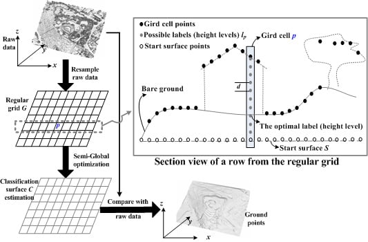
SGF tries to identify an approximate ground surface (called classification surface) from discrete height levels at the horizontal grid cells of data. To achieve this objective, SGF performs three major operations: (1) forms discrete grid data from the raw point data and sets up possible height levels (labels) of each grid cell; (2) applies semi-global optimization to determine the optimal height level (label) of each grid cell, through which the classification surface is obtained; and (3) uses the classification surface to categorize the raw point data into ground and non-ground points.
Figure 1 shows the workflow of SGF. The raw point data is first discretized into a regular grid G. For each grid cell p = (x, y), the grid cell point Gp is taken as the lowest elevation of all points within this grid cell. The empty cells without points are left blank and ignored during subsequent processing. The resolution of G is related to the density of the raw point data. As illustrated in the section view of Figure 1, the set of height levels for each grid cell lp is defined as:
l p = { l p i | l p i = S p + i × d } i = 0 N where  N = [ ( G p S p ) / d ]
where d is the unit height and N is the number of possible height levels in grid cell p. Sp is the height of grid cell p from the start surface S. The start surface is a horizontal plane with height that is equal to the lowest elevation of all points in the raw point data.
Considering a regular grid G of size W × H, SGF can be represented as a labeling problem in which the labels correspond to different height levels. As illustrates in the section view of Figure 1, the optimization procedure of SGF aims to assign an optimal label for each grid cell. This optimal label is the approximate ground height. To avoid clutter in subsequent sections, height levels are represented as labels. SGF optimizes the energy function as follows:
l * = arg min l E ( l ) = arg min l ( γ E d a t a ( l ) + E r e g ( l ) )
where l is the set of possible labels for all grid cells, and l* denotes the optimal labels that minimize energy function E(l). The optimal labels l* form a classification surface C, based on which the raw points are classified as either ground or non-ground. The data term Edata(l) and regularization term Ereg(l) are balanced by ground saliency γ, which is discussed in the following section. Details about the data term and regularization term are presented in Section 2.3. For convenience in description, the desired DTM accuracy is defined as Da.
Figure 1. Workflow of SGF algorithm and the section view of a row from the regular grid (to avoid clutter, we draw possible labels for only one grid cell).
Remotesensing 07 10996 g001
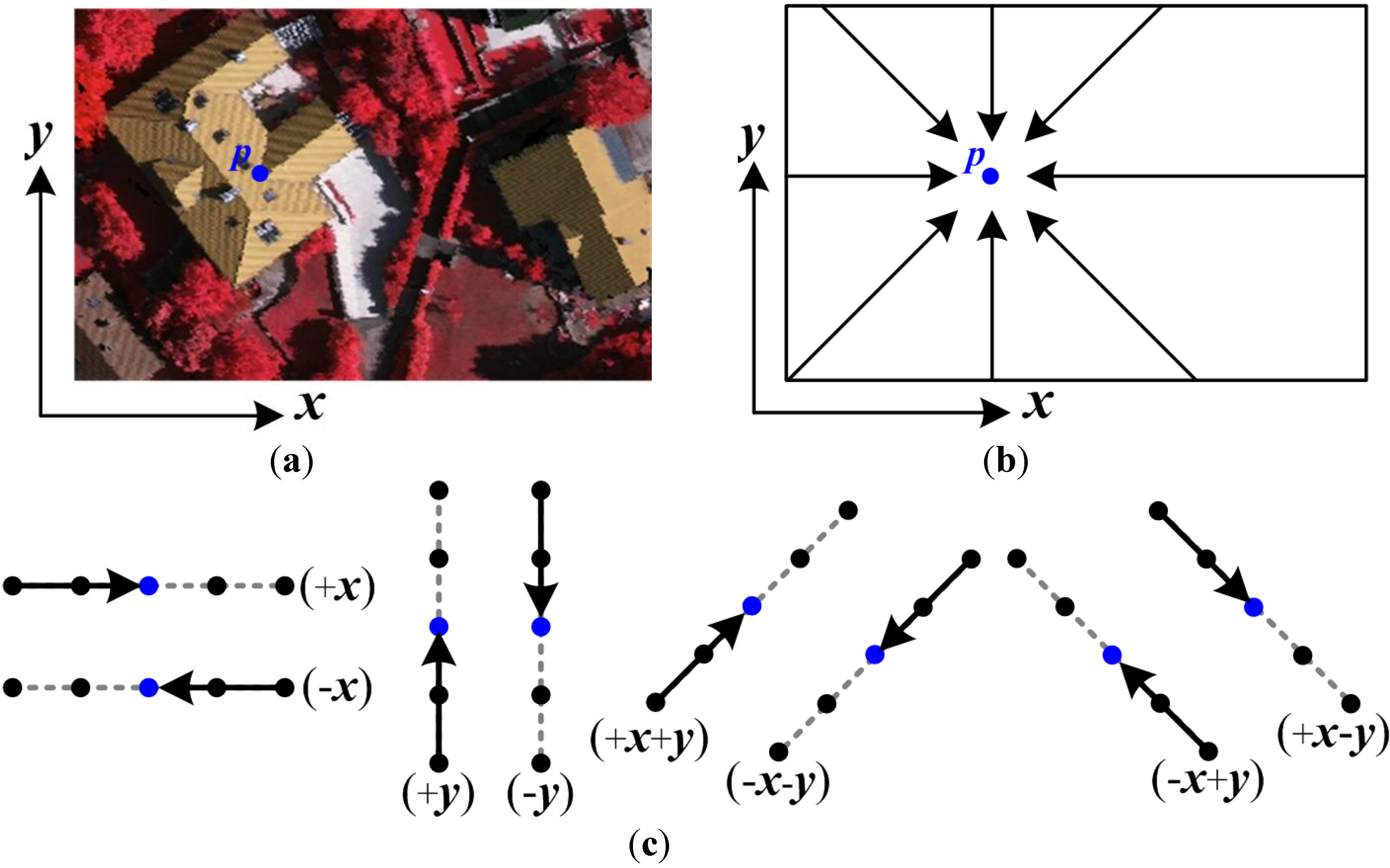
As mentioned in the Introduction, energy function is equally optimized in a 1D manner from all directions. Figure 2 demonstrates that eight independent directions (Figure 2b) are used to assign each grid cell p (Figure 2a) with a label l lp. These directions are +x, −x, +y, −y, +x+y, −x−y, +x−y and −x+y (Figure 2c). It is noteworthy that all the subsequent sections operate over these eight independent directions equally.
Figure 2. Optimization directions: (a) a regular grid grayed by the corresponding image; (b) and (c) eight optimization directions used in SGF.
Remotesensing 07 10996 g002

2.2. Computation of Ground Saliency for Adaptively Balancing the Energy Function
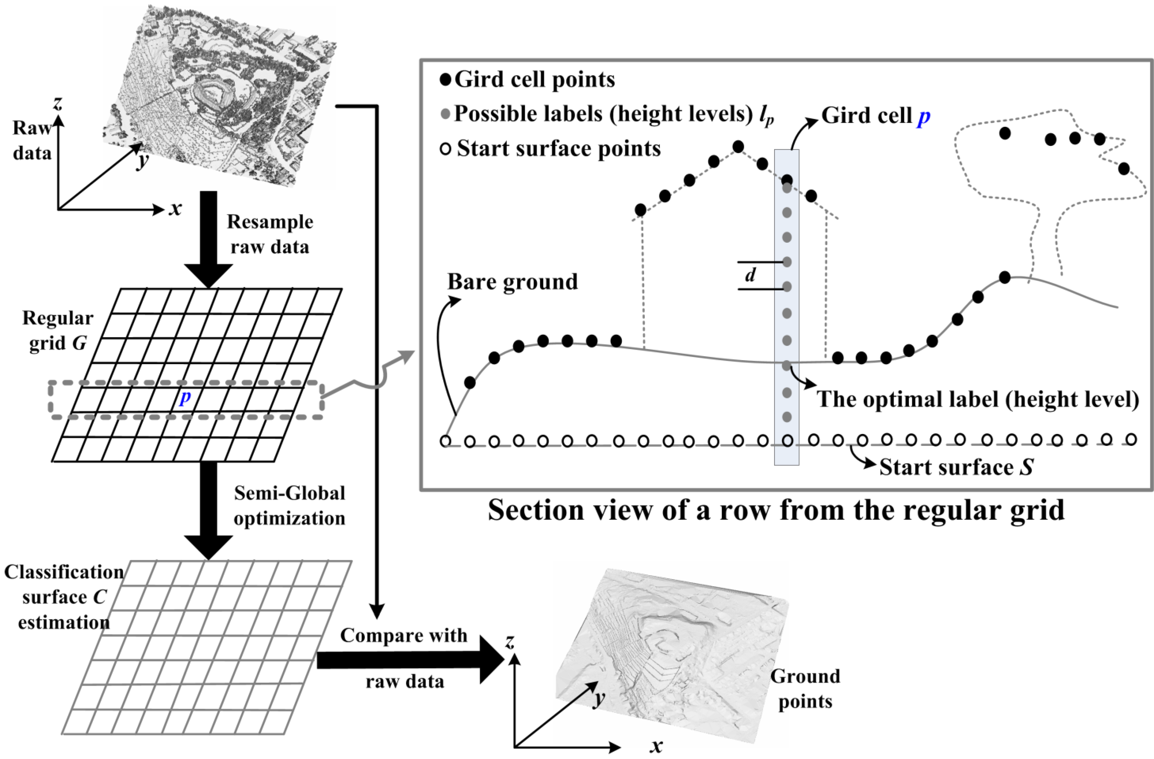
Optimization methods often define energy function with a data term and a regularization (smoothness) term balanced by a constant coefficient [22,23,29]. LiDAR filtering algorithm segments height differences to roughly detect the local saliency of ground features because abrupt height changes indicate a high possibility that the features are non-ground. In this paper, we use ground saliency γ to adaptively reconcile the energy function (2). At the onset of the experiment, the ground saliency γp for each grid cell p is set as 1.0 γp is then updated by two steps: segmentation and subtraction. Without loss of generality, assume that we are sweeping the window from left to right for a given row y in the regular grid G. The grid cell point Gp is first segmented into segments according to the height difference with the grid cell point before it. Figure 3 illustrates the segmentation procedure for a given row when the window is swept from left to right. If the segment has a significant height discontinuity with the segment that comes after it, then the ground saliencies of all grid cells in this segment subtract a constant value of 0.125 (=1.0/N, N is the number of directions (i.e., eight directions in this paper)). Figure 4 displays a simulated example of the subtraction procedure for a given row when the window is swept from left to right and from right to left. The segmentation threshold Sthro in Figure 3 is equal to Da and the subtraction threshold Gthro in Figure 4 is equal to 3 × Da. The segmentation and subtraction procedures are conducted in all eight crossing directions independently as shown in Figure 2. These steps operate extremely fast because they only perform simple computation (height comparison).
Figure 3. Cross section of the segmentation procedure when the window is swept from left to right: (a) cross section of a given row from the regular grid; (b), (c) and (d) grid cell points are segmented into different segments according to height difference with the grid cell points before them; and (e) segmentation result.
Remotesensing 07 10996 g003
Figure 4. Cross section of the subtraction procedure: (a), (b) and (c) segment has a significant height discontinuity with the segment after it in this sweep direction (left to right), the ground saliencies of all grid cells in this segment subtract a constant value (0.125) in this simulated example; (d), (e) and (f) show the similar operation from right to left.
Remotesensing 07 10996 g004
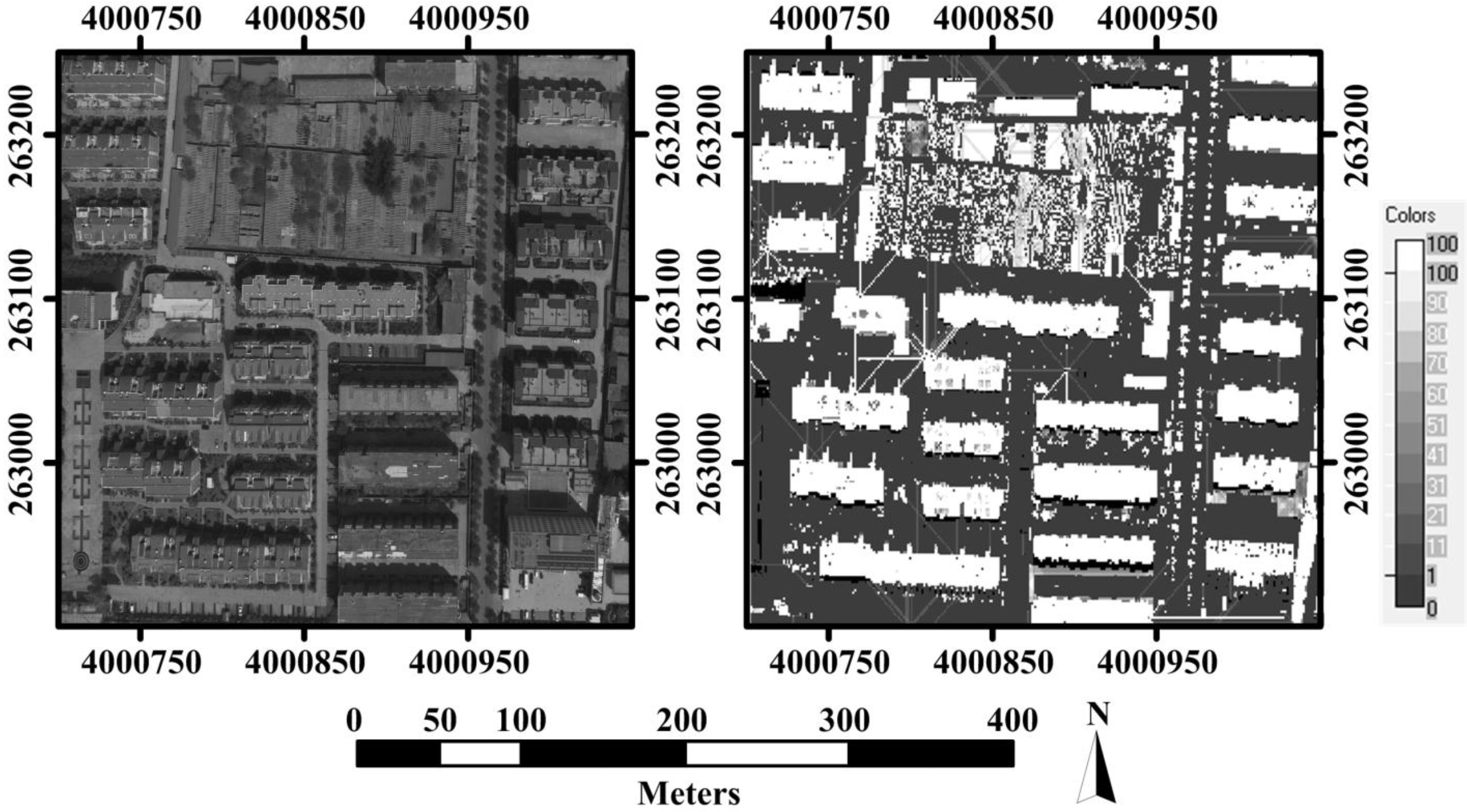
Each grid cell has a unique ground saliency calculated according to the height differences between grid cell points. The ground saliency has nothing to do with the possible labels. Figure 5 exhibits an example of ground saliency results. Both the building and vegetation cells are highlighted, and they have relatively small ground saliencies (Figure 5b). The calculation of ground saliency does not mean a precise classification of each grid cell. Instead, it is used to adaptively balance the energy terms in (2) other than using a constant coefficient. Given that the building and vegetation cells have relatively small (even 0) ground saliencies, the regularization term (in Equation (2)) of these places is dominant. This case can prevent the classification surface from being attracted to large low buildings and vegetation.
Figure 5. Ground saliency results: (left) is the corresponding image of point cloud (right); (right) is grayed by (1.0 − γp) × 100.
Remotesensing 07 10996 g005

2.3. Semi-Global Optimization

2.3.1. Semi-Global Matching
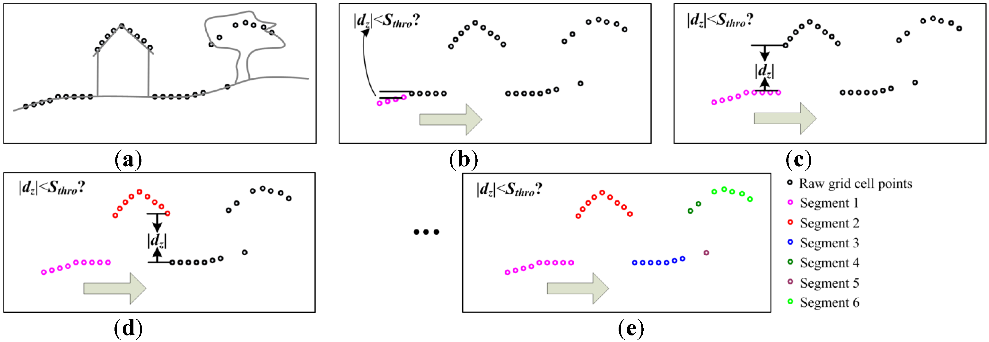
Semi-Global Matching is an efficient algorithm for dense stereo matching [25,30,31,32]. The energy function of SGM can also be expressed as (2). SGM divides global optimization into multiple 1D optimization processes, which are straight lines that run through the image in multiple directions (Figure 6). Each direction is performed separately, the costs are then summed to choose a labeling (in stereo: disparity map) for the image [32]. Let Lr be a path that is traversed in the direction r. The cost Lr(Dp) of pixel p at disparity D is defined recursive as:
L r ( D p ) = φ ( D p ) + min D p r { L r ( D p r ) + φ ( D p r , D p ) }
where φ(Dp) is the data term (matching cost) defined by Mutual Information (MI), and φ(Dp-r, Dp) is the regularization term (smoothness cost) defined over the edge.
The aggregation of directional costs is summed in all directions r:
S ( D p ) = r L r ( D p )
Finally, a pixel label is obtained by defining:
D p S G M = arg min D p S ( D p )
Above is a simple generalization of SGM described by Hirschmüller and more details can be found in [25,28].
Figure 6. Cost aggregation of SGM: (a) minimum cost path in disparity space; and (b) eight directions that go through the red pixel p.
Remotesensing 07 10996 g006

2.3.2. Cost Aggregation of SGF

The data term in (2) is the filtering cost expressed by a function of the distance between Gp and a given label l lp:
E d a t a ( l ) = 1.0 e ( G p l ) 2
This function makes the optimal labels (classification surface) attracted to G. Such an attraction force is strong if the label is close enough to a true ground cell point. The grid cell points belong to non-ground objects leave the classification surface unaffected. As shown in Figure 7a, the grid cell points from vegetation and buildings are too far from the classification surface to attract it.
The regularization term is the path cost calculated from the labels of neighboring grid cells:
E r e g ( l ) = { | arctan ( l p l q ) |      if | l p l q | π 2 | l p l q |                    otherwise 
Figure 7. (a) Cross-section of a scene: the classification surface is attracted to the ground while the tree and building points are too far to attract the classification surface; (b) q is the grid cell before p along a direction.
Remotesensing 07 10996 g007
Unlike the traditional 4-connected and 8-connected neighborhoods, q in this case refers to the grid cell before p along a direction (Figure 7b). This term adds small and large penalties to labels with little or great elevation changes, respectively. A small penalty for small elevation changes permits an adaptation to a gentle slope. Contrarily, a large penalty for large elevation changes preserves steep terrains, such as terraced fields and scarps.
Optimization procedure aims to determine an optimal label, which minimizes energy function (2), for each grid cell. The off-the-shelf solvers for identifying the minimum of global energy function differ. The directional optimization method DP [33,34] minimizes the energy function along each direction individually. However, DP solutions easily suffer from streaking [25]. The high-performing methods, including Graph Cuts [35] and Belief Propagation [36,37,38], operate in two dimensions (2D). The layered [36,37,39] and Block Coordinate Descent (BCD) approaches [24] are iteratively optimized. This paper minimizes the energy function E(l) via semi-global optimization, which is inspired by SGM [25,28]. A comparative study (http://vision.middlebury.edu/stereo) revealed that the semi-global optimization methods are not as accurate as state-of-the-art ones in solving the stereo matching of indoor scenes. Nevertheless, the semi-global optimization is faster and more robust than most other approaches, particularly when dealing with aerial data [30].Semi-global optimization performs cost aggregation as an approximation of the global optimization via DP from eight directions (Figure 2b). The cost C(p, l) for a grid cell p and a label l lp is calculated by summing the costs of eight minimum cost directions that end in grid cell p at label l lp. Only the path cost of DP is required rather than the path itself. Finally, the label of each grid cell with the lowest total cost is selected to form the final classification surface. This semi-global optimization does not iterate and only converges at the summation of eight directional minimal costs.
The quality and computation performance of semi-global optimization are compared with those of the state-of-the-art approaches via BCD, a fast MRF solver [24], to optimize energy function (2). BCD has been proved fast and trivially parallelizable when dealing with global optimization problems [24]. As this algorithm is iteratively optimized, the regularization term (4) should be changed into the following form:
E r e g ( l ) = q N p { | arctan ( l p l q ) |      if | l p l p | π 2 | l p l q |                    otherwise 
where Np is the 4-connected neighborhood. The results are shown in Section 3.

2.4. GPU Acceleration of SGF Algorithm
SGF divides global optimization into multiple 1D optimization processes. Different 1D paths run at different directions to approximate a global optimization. Each line and direction is executed independently, implying that SGF can be paralleled via GPU. This semi-global optimization proposes a new alternative technique that achieves results similar to those of global methods while maintaining a reduced execution time [40]. In this paper, Compute Unified Device Architecture (CUDA) [41] is used to implement parallel computing in GPU.
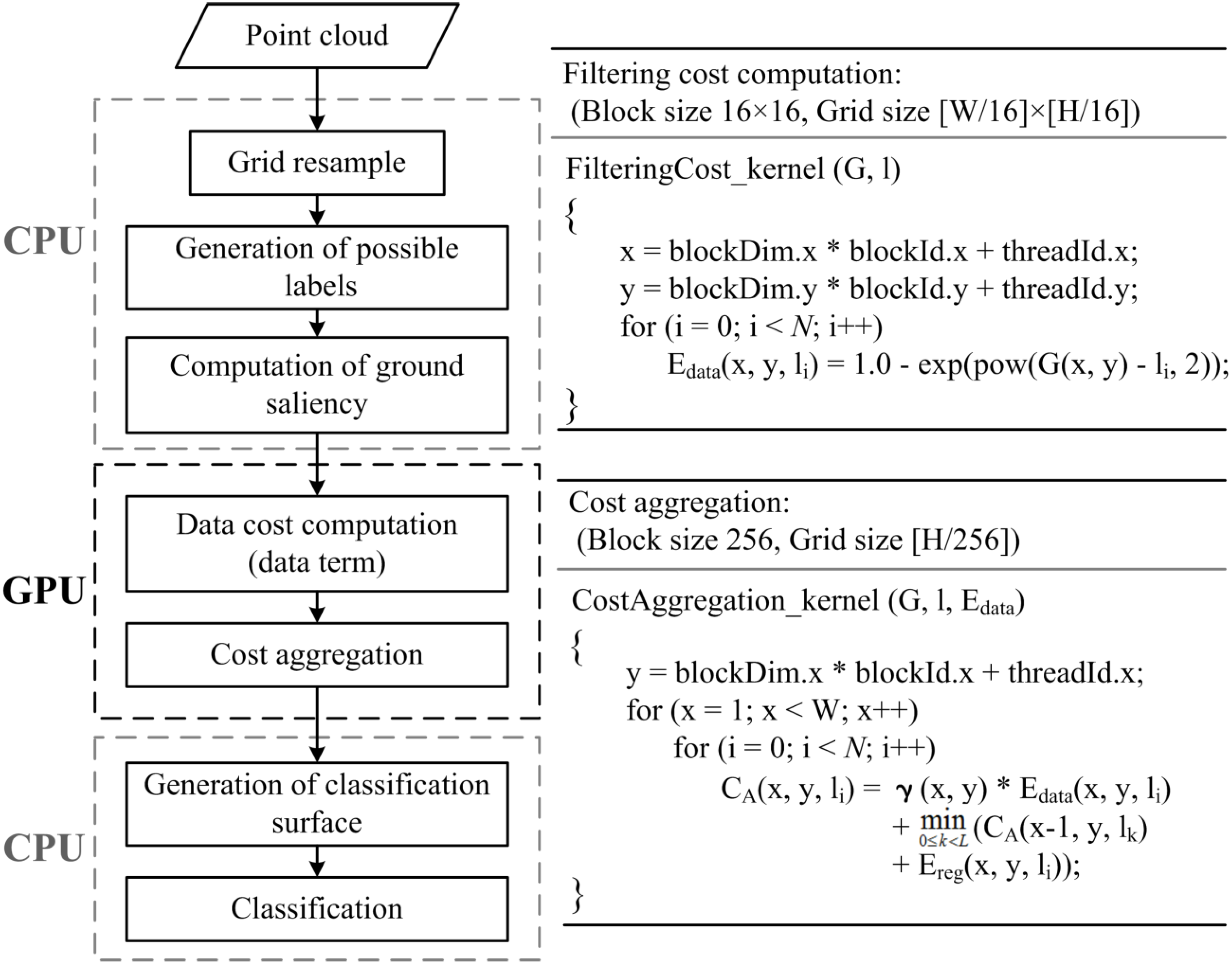
Figure 8 demonstrates that the filtering cost (data term of (3)) computation and cost aggregation are executed in various threads of GPU. The other procedures, including grid resample, generation of possible labels, computation of ground saliency, generation of classification surface, and classification, are implemented in Central Processing Unit (CPU). In our implementation, eight cost aggregation kernels corresponding to eight directions are designed. The cost aggregation kernel shown in Figure 8 is an example of direction +x, where N is the number of possible labels in each grid cell.
Figure 8. (Left) workflow of GPU acceleration, (right) implementation of the GPU kernels.
Remotesensing 07 10996 g008

2.5. Point Filtering and Parameter Setting

Point filtering (classification) is performed by comparing the raw data with the generated classification surface. The points close enough (i.e., half of the desired DTM accuracy Da) to this surface are classified as ground points.
There are five parameters in the proposed SGF, including the desired DTM accuracy Da, the resolution of the regular grid G, the unit height d, the segmentation threshold Sthro, and the subtraction threshold Gthro. The desired DTM accuracy Da is set according to the needs of the users. In Section 3, the desired DTM accuracy is 0.5 m. The resolution of the regular grid is equal to the area of the raw data coverage divided by the number of points. The segmentation threshold is equal to Da and the subtraction threshold is 3 × Da.
To form a fine classification surface, the unit height d in (1) should be as small as possible. However, SGF may suffer from unacceptable computation cost and memory consumption because the set of possible labels is huge. To solve this problem, the SGF algorithm is performed twice. In the first execution, the unit height d is set as a relative large value (i.e., 5 m). In the second execution, the unit height d is set as a small value (i.e., half of Da) and the possible labels for each grid cell l p are then recalculated as follows:
l p = { l p i | l p i = l p * + i × d } i = 0 N where  N = [ ( G p l p * ) / d ]
where l p * is the optimal label that selected in the first execution. A few possible labels exist in the second execution because l p * is close to the bare ground.

3. Experimental Results and Discussion

3.1. Quality Assessment on ISPRS Test Data Set

We first apply the SGF algorithm to the benchmark dataset provided by the International Society for Photogrammetry and Remote Sensing (ISPRS) Commission III/WG3 (http://www.commission3.isprs.org/wg3/) and compare the filtering accuracy of SGF with those of eight classical filtering methods [2], parameter-free algorithm [1], Terrasolid TerraScan, and BCD. The ISPRS dataset is composed of 15 samples with different terrain features and point spacing. The details of this dataset are presented in [2]. Each sample is considered “difficult” for filtering [2]. Filtering accuracy is measured by considering the Type I error, which is the percentage of rejected bare ground points; the Type II error, which is the percentage of accepted non-ground points; and the total error, which is the overall probability of points being incorrectly classified.
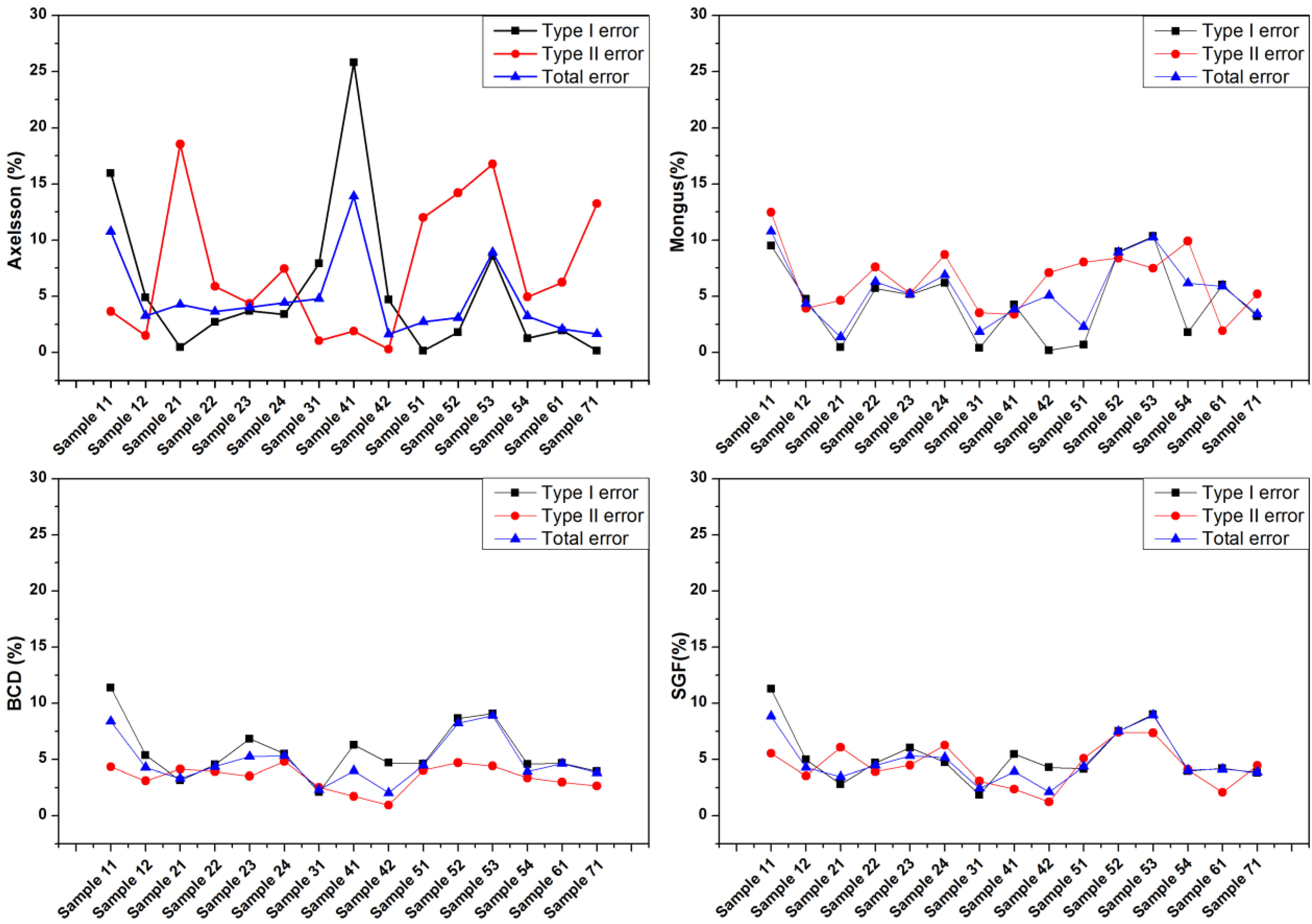
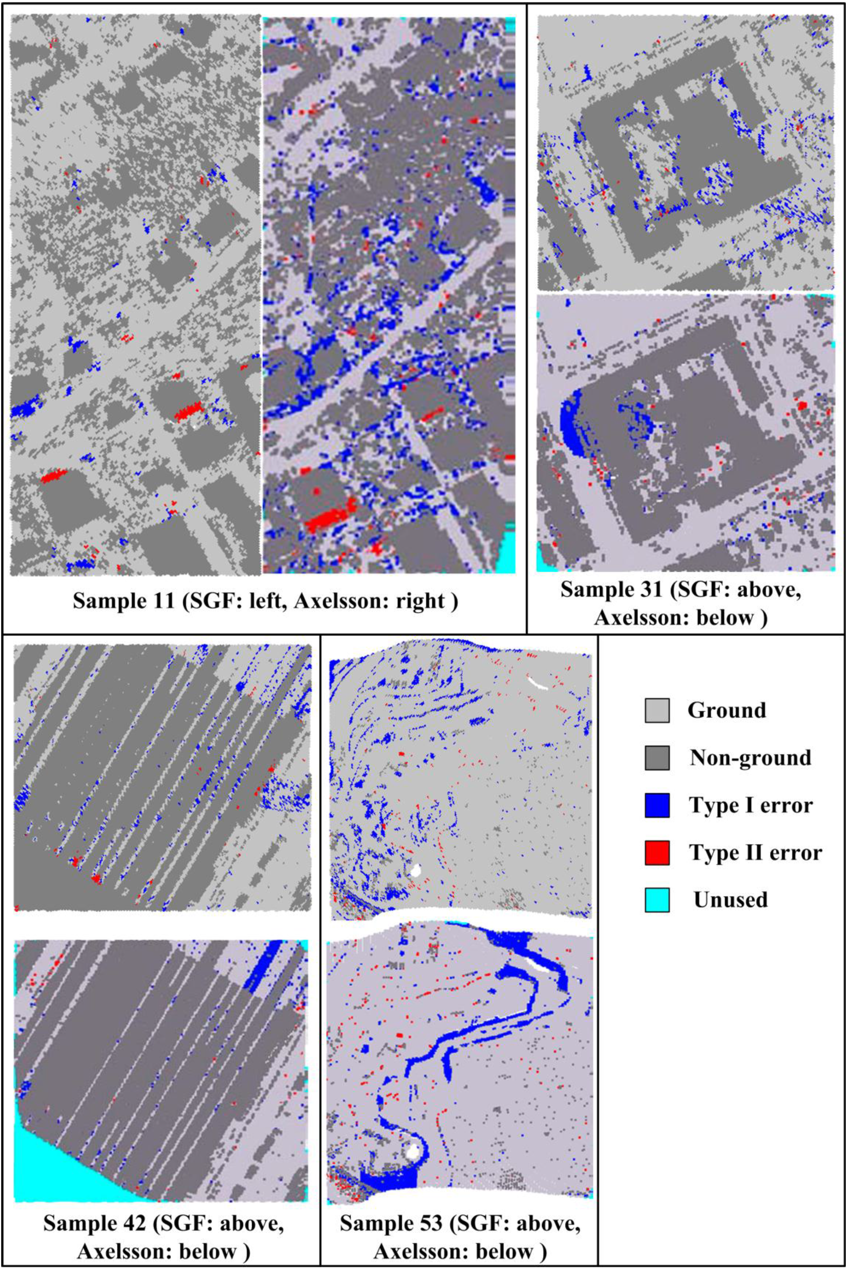
The eight classical filtering methods were published in 2004 and there have been improvements in them since then. We also compare our results with the state-of-the-art parameter-free algorithm [1] and the most popular commercial software TerraSolid TerraScan. TerraScan uses the TIN-based filtering method. This software produces a significantly low average total error when a set of tunable parameters of the data is passed to the algorithm [42]. Compared with the tested algorithms, the proposed SGF produces the second type I error and total error, as indicated in Table 1. The low type I error indicates that using SGF can properly maintain the terrain details. The average total error of SGF ranks second and is very close to the best one (4.85% of SGF vs. 4.82% of Axelsson). This situation can be attributed to the integrated use of ground saliency computed via the segmentation of height differences and the well-defined energy function, which properly combines all information into the framework of the semi-global optimization. Figure 9 shows a detailed comparison with Axelsson’s algorithm [14], parameter-free method (Mongus), BCD, and the proposed SGF algorithm across the 15 samples. The results indicate that although the total average error of SGF is only slightly higher than that of Axelsson’s algorithm, the SGF and BCD yield more consistent accuracy over different samples, showing the tendency of better stability. Sample31 and Sample42 have the lowest total errors while Sample11 and Sample53 have the highest total errors for SGF. Figure 10 shows the error distribution of the SGF and Axelsson’s algorithm on Sample11, Sample31, Sample42 and Sample53. Although SGF and Axelsson’s algorithm have very close average total error, they exhibit different error distributions. SGF produces more sparse distributions of error points while Axelsson’s algorithm yields more clusters of type I error (see Sample11 and Sample 53), which may result in the loss of important terrain features in the DTM.
Table 1. Comparison of average accuracy among the eight classical filtering methods, parameter-free method (Mongus), TerraScan, BCD, and the proposed SGF algorithm for all benchmark study samples (the number in boldface indicates the smallest value in each error type, implying the corresponding method has the best performance).
Type I Error (%)Type II Error (%)Total Error (%)
Elmqvist39.431.9620.73
Sohn9.948.599.35
Axelsson5.557.464.82
Pfeifer10.823.328.02
Brovelli36.771.8825.78
Roggero17.123.1112.35
Wack16.521.5812.04
Sithole24.592.0817.48
Mongus4.56.55.49
TerraScan11.054.527.61
BCD5.693.414.88
SGF5.254.464.85
Figure 9. Detailed comparison of Axelsson’s algorithm, parameter-free method (Mongus), BCD, and the proposed SGF algorithm across 15 samples.
Remotesensing 07 10996 g009
Figure 10. Error distribution of SGF and Axelsson’s algorithm on Sample11, Sample31, Sample 42, and Sample53.
Remotesensing 07 10996 g010

3.2. Computational Performance

The algorithm has been implemented for using CPU and GPU by C++ under the Microsoft Windows 7 operating system. A personal computer with Intel Core i7 3.6GHz CPU, 8GB memory, and an NVIDIA GeForce GTX690 GPU with 3072 stream processors is used for testing. The second data set, which is obtained from the city of Foshan in Guangdong Province of China, is selected to evaluate the computational performance. This dataset includes steep slopes, discontinuities, complex scenes, and outliers, which are considered difficult for filtering [2]. The point density is 0.94 points/m2.
SGF checks each LiDAR point in its eight cardinal directions independently. Such a property allows GPUs to be utilized efficiently. Other methods, including TIN-based methods, interpolation-based methods, and global optimization-based methods, classify each LiDAR point according to the attributes calculated from the neighboring points to a relatively large extent. Such properties make these algorithms unable to be parallelized or, at least, not parallelized in an easy way. TerraScan is used to compare the CPU performance, and BCD is adopted to compare the CPU and GPU performance. Table 2 indicates that compared with TerraScan, the proposed method saves almost 60% of CPU time. For the GPU-accelerated SGF, a processing speed of approximately 3 million points per second is achieved, making this method approximately three times faster than BCD. The reason for this condition is that BCD needs to run about 5–7 times over two directions while considering 4-connected neighborhoods, whereas SGF runs 1–2 times over eight directions. The experiments reveal that SGF is useful when a highly-efficient DTM production is needed, such as mapping for large areas, disaster response, and real-time site inspection.
Table 2. Comparison of computational performance between TerraScan, BCD, and SGF.
Test DatasetSampleSample1Sample2Sample3Sample4Sample5
Number of Points (million)5.410.324.340.248.6
TerraScanCPU (s)15.131.475.8115.4140.3
GPU (s)*****
BCDCPU (s)28.2460.53148.69224.85278.91
GPU (s)5.329.2522.4732.5441.61
SGFCPU (s)9.6719.2144.5475.3889.62
GPU (s)1.913.528.1112.3615.42
* TerraScan tested cannot be executed in GPU mode.

3.3. Discussion

In this section, some of the difficult terrains in the test data are discussed to validate the proposed method. The free software FugroViewer (http://www.fugroviewer.com/) is used to create the gray images rendered on the triangulated DTMs.
Case 1: Steep slopes
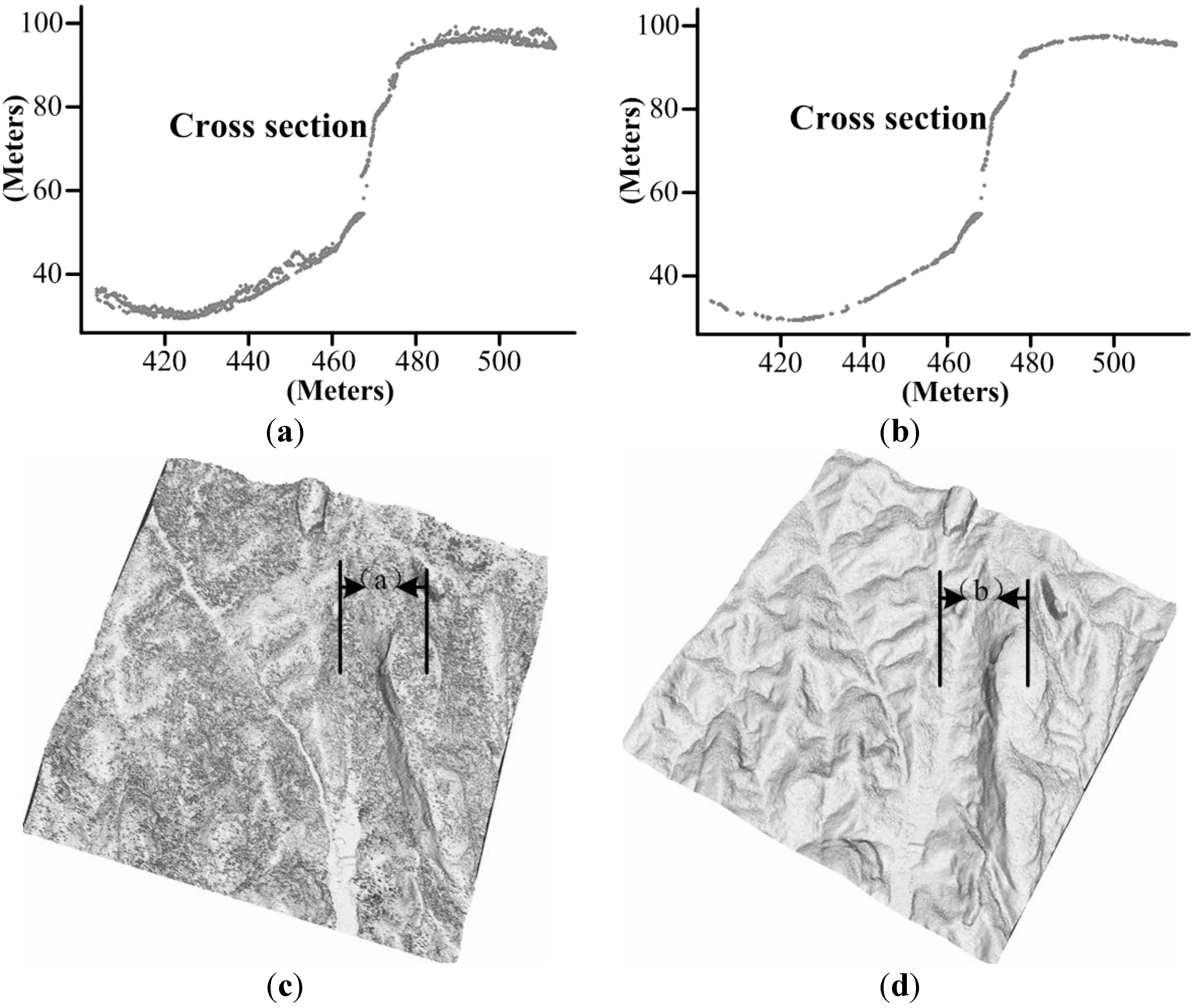
As previously mentioned, steep slopes and discontinuities are difficult to handle when separating bare ground and objects. Therefore, points with significant height differences from their neighbors are assumed to be non-ground objects. This assumption may not be true when the terrain slope is high. Considering that the proposed method optimizes a cost function, which adds a small penalty for points on gentle slopes and a large penalty for points on steep slopes (4), the method permits both small and large height differences. The test results show that SGF can preserve steep slopes (Figure 11).
Case 2: Discontinuities
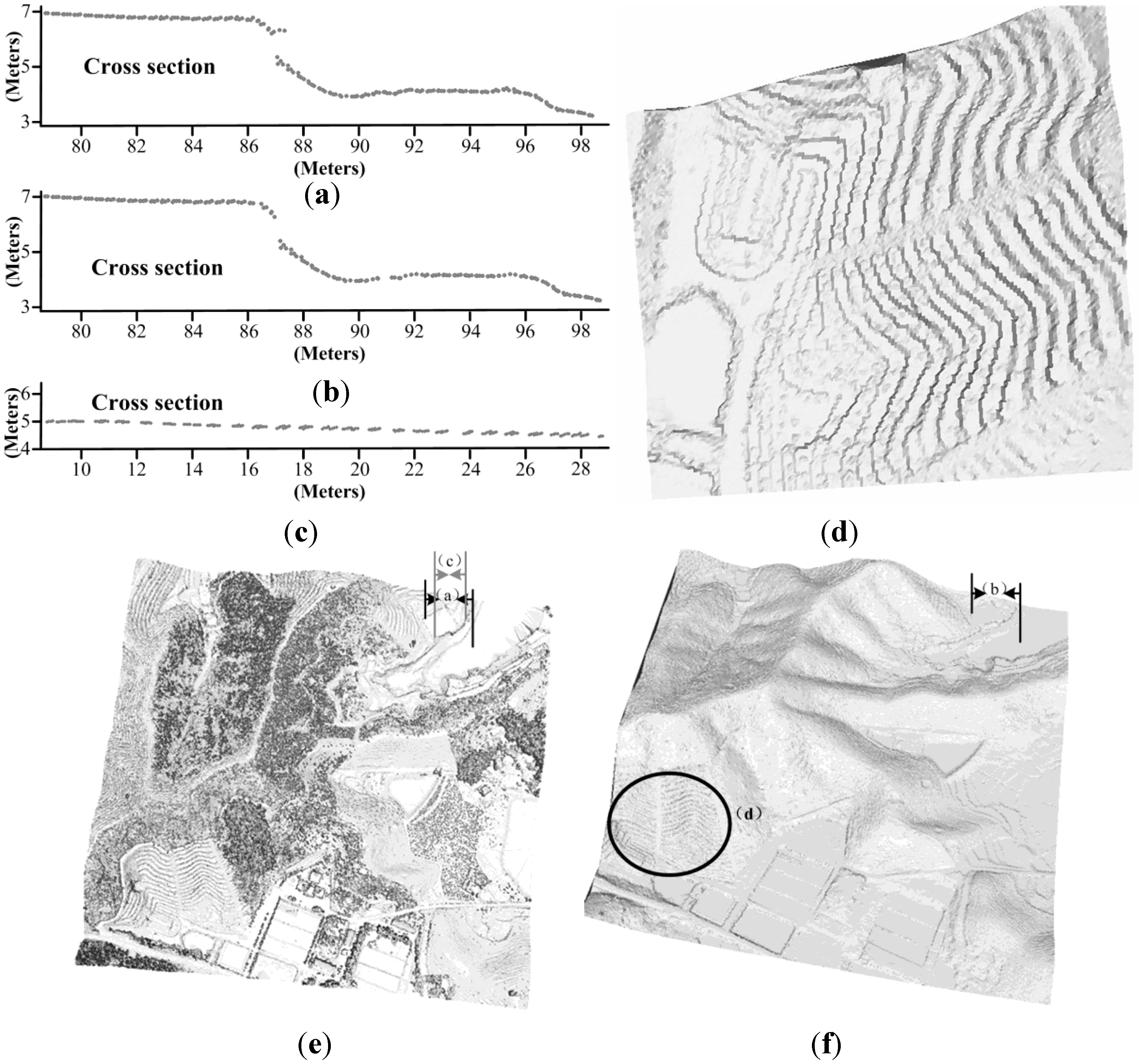
Generally, objects can be filtered out because they are discontinuous from the bare ground. However, breaklines on the bare ground are an exception to this assertion [2]. These discontinuities should be preserved for high-quality DTM generation. These kinds of discontinuity are not continuous in the 2D view (Figures 12a,b), but they may be continuous from some directions in 1D view (Figure 12c). Since the cost function of SGF is optimized from eight directions, the final classification surface is selected by the information provided from all these directions. This case implies that the breaklines may not be detected from one direction (Figure 12a), but they can be detected from other directions (Figure 12c). The results are presented in Figure 12.
Case 3: Complex objects
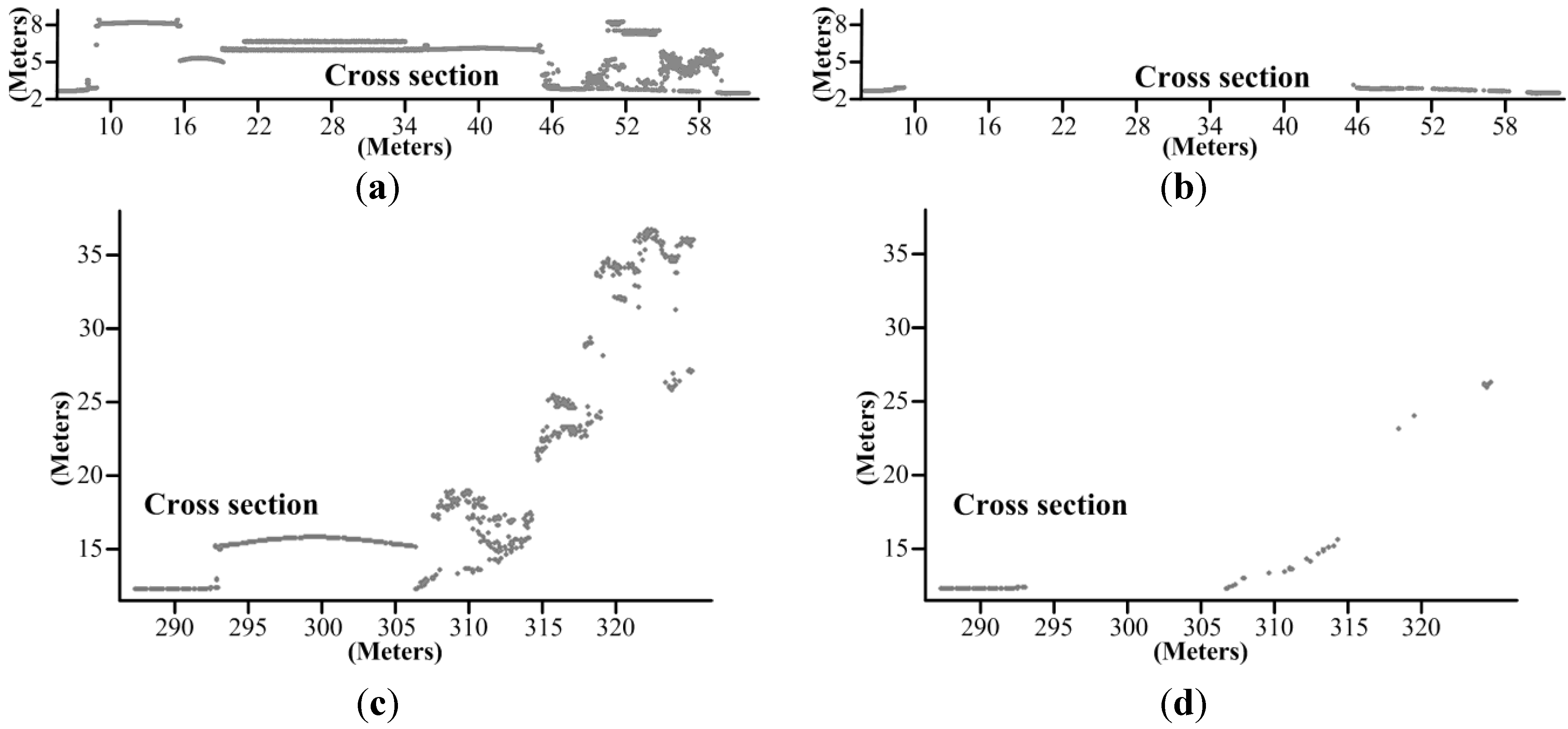
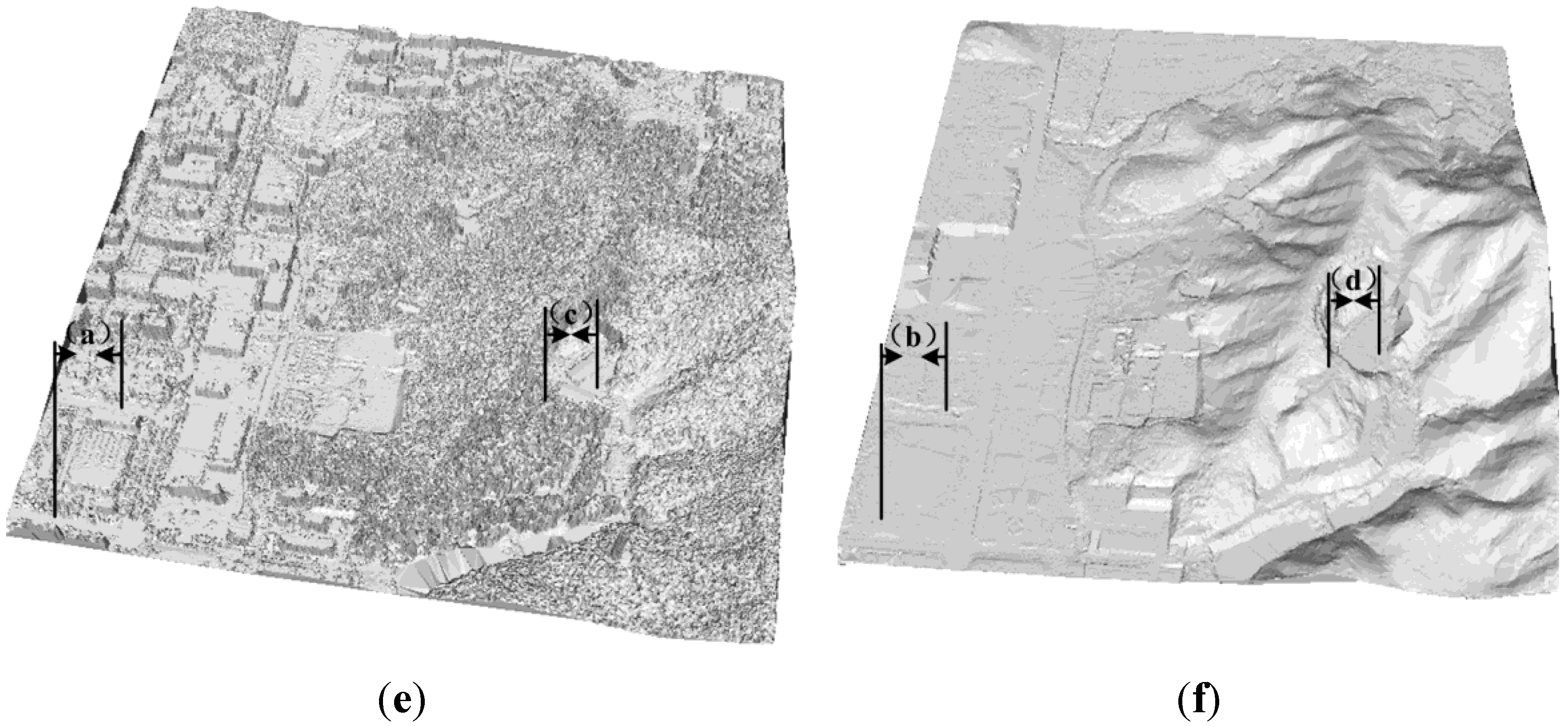
Complex objects (e.g., large, low (Figure 13a), and attached (Figure 13c)) are difficult to separate from bare ground. Given that both the local elevation difference and global information of the point cloud are considered, and the point cloud is pre-classified by the ground saliency, SGF can remove complex objects. The ground saliency calculation step is essentially a segmentation algorithm by which building roofs and areas with breaklines can be segmented. When the segmented information is integrated into the optimization function (2), it enables a better selection of the classification surface to deal with the combination of vegetation, buildings, and steep terrains. Some examples of complex object removal are shown in Figure 13.
Figure 11. Preservation of steep slope: (a) and (b) are the cross sections; (c) is the raw point data; (d) is the DTM generated by SGF.
Remotesensing 07 10996 g011
Figure 12. Preservation of terrain discontinuities: (a), (b) and (c) are cross sections; (d) is the terrain details; (e) is the raw point data; (f) is the DTM generated by SGF.
Remotesensing 07 10996 g012
Figure 13. Removal of complex objects: (a), (b), (c), and (d) are cross sections; (e) is the raw point data; (f) is the DTM generated by SGF.
Remotesensing 07 10996 g013aRemotesensing 07 10996 g013b

4. Conclusions

This paper proposes a novel SGF algorithm that can efficiently classify the ground and non-ground points over various complex scenes. The classification accuracy of this algorithm is almost the best one (second place on overall error rate) based on the standard benchmark datasets, but it runs fast and produces competitive results. Semi-global optimization balances the quality and computational cost well. This undertaking can be easily achieved via parallel computing because of its independent computation along different directions. SGF can achieve a speed of approximately 3 million points per second via GPU computing. Overall, SGF is a fast and intelligent filtering algorithm that can process large volumes of data with good classification accuracy. Thus, this algorithm has significant potential for generating DTMs from airborne LiDAR data.

Acknowledgments

This study was partially supported by the National Key Basic Research and Development Program (Project No. 2012CB719904) of China, Guangzhou City funding of science and technology (Project No. 201508020054) and the funding of the workstation of Chinese Academicians by Guangdong province. The authors thank Guangzhou Jiantong Surveying, Mapping and Geographical Information Technology Development Ltd. for providing the data used in this research. Junfeng Zhu conducted initial experimental study on dynamic-programming-based filtering.

Author Contributions

Xiangyun Hu proposed to use semi-global optimization for filtering and revised the paper. Lizhi Ye designed the algorithm and performed the experiments, he also wrote the paper. Shiyan Pang conducted the initial study on dynamic-programming-based filtering. Jie Shan revised the paper.

Conflicts of Interest

The authors declare no conflicts of interest.

References

  1. Mongus, D.; Žalik, B. Parameter-free ground filtering of LiDAR data for automatic DTM generation. ISPRS J. Photogramm. Remote Sens. 2012, 67, 1–12. [Google Scholar] [CrossRef]
  2. Sithole, G.; Vosselman, G. Experimental comparison of filter algorithms for bare-Earth extraction from airborne laser scanning point clouds. ISPRS J. Photogramm. Remote Sens. 2004, 59, 85–101. [Google Scholar] [CrossRef]
  3. Liu, X. Airborne LiDAR for DEM generation: some critical issues. Prog. Phys. Geog. 2008, 32, 31–49. [Google Scholar]
  4. Vosselman, G. Slope based filtering of laser altimetry data. Int. Arch. Photogramm. Remote Sens. 2000, 33, 935–942. [Google Scholar]
  5. Shan, J.; Aparajithan, S. Urban DEM generation from raw LiDAR data. Photogramm. Eng. Remote Sens. 2005, 71, 217–226. [Google Scholar] [CrossRef]
  6. Meng, X.; Wang, L.; Silván-Cárdenas, J.L.; Currit, N. A multi-directional ground filtering algorithm for airborne LiDAR. ISPRS J. Photogramm. Remote Sens. 2009, 64, 117–124. [Google Scholar] [CrossRef]
  7. Susaki, J. Adaptive slope filtering of airborne LiDAR data in urban areas for digital terrain model (DTM) generation. Remote Sens. 2012, 4, 1804–1819. [Google Scholar] [CrossRef] [Green Version]
  8. Kraus, K.; Pfeifer, N. Determination of terrain models in wooded areas with airborne laser scanner data. ISPRS J. Photogramm. Remote Sens. 1998, 53, 193–203. [Google Scholar] [CrossRef]
  9. Pfeifer, N.; Reiter, T.; Briese, C.; Rieger, W. Interpolation of high quality ground models from laser scanner data in forested areas. Int. Arch. Photogramm. Remote Sens. 1999, 32, 31–36. [Google Scholar]
  10. Lee, H.S.; Younan, N.H. DTM extraction of LiDAR returns via adaptive processing. IEEE Trans. Geosci. Remote Sens. 2003, 41, 2063–2069. [Google Scholar] [CrossRef]
  11. Zhang, K.; Chen, S.; Whitman, D.; Shyu, M.; Yan, J.; Zhang, C. A progressive morphological filter for removing nonground measurements from airborne LiDAR data. IEEE Trans. Geosci. Remote Sens. 2003, 41, 872–882. [Google Scholar] [CrossRef]
  12. Chen, Q.; Gong, P.; Baldocchi, D.; Xie, G. Filtering airborne laser scanning data with morphological methods. Photogramm. Eng. Remote Sens. 2007, 73, 175–185. [Google Scholar] [CrossRef]
  13. Mongus, D.; Lukač, N.; Žalik, B. Ground and building extraction from LiDAR data based on differential morphological profiles and locally fitted surfaces. ISPRS J. Photogramm. Remote Sens. 2014, 93, 145–156. [Google Scholar] [CrossRef]
  14. Axelsson, P. DEM generation from laser scanner data using adaptive TIN models. Int. Arch. Photogramm. Remote Sens. 2000, 33, 111–118. [Google Scholar]
  15. Sohn, G.; Dowman, I.J. Terrain surface reconstruction by the use of tetrahedron model with the MDL criterion. Int. Arch. Photogramm. Remote Sens. 2002, 34, 336–344. [Google Scholar]
  16. Kang, X.; Liu, J.; Lin, X. Streaming progressive TIN densification filter for airborne LiDAR point clouds using multi-core architectures. Remote Sens. 2014, 6, 7212–7232. [Google Scholar] [CrossRef]
  17. Sithole, G.; Vosselman, G. Filtering of airborne laser scanner data based on segmented point clouds. Int. Arch. Photogramm. Remote Sens. 2005, 36, 66–71. [Google Scholar]
  18. Tóvári, D.; Pfeifer, N. Segmentation based robust interpolation-a new approach to laser data filtering. In Proceedings of the ISPRS Workshop Laser scanning 2005, Enschede, The Netherlands, 12–14 September 2005.
  19. Tolt, G.; Persson, Å.; Landgård, J.; Söderman, U. Segmentation and classification of airborne laser scanner data for ground and building detection. In Proceedings of the Defense and Security Symposium, Orlando, FL, USA, 17 April 2006.
  20. Meng, X.; Currit, N.; Zhao, K. Ground filtering algorithms for airborne LiDAR data: A review of critical issues. Remote Sens. 2010, 2, 833–860. [Google Scholar] [CrossRef]
  21. Elmqvist, M. Ground surface estimation from airborne laser scanner data using active shape models. Int. Arch. Photogramm. Remote Sens. 2002, 34, 114–118. [Google Scholar]
  22. Zhou, Q.; Neumann, U. Complete residential urban area reconstruction from dense aerial LiDAR point clouds. Graph. Models 2013, 75, 118–125. [Google Scholar] [CrossRef]
  23. Verdie, Y.; Lafarge, F.; Alliez, P. LOD Generation for urban scenes. Acm. Trans. Graph. 2015, 34, 15–29. [Google Scholar] [CrossRef]
  24. Chen, Q.; Koltun, V. Fast MRF optimization with application to depth reconstruction. In Proceedings of the Computer Vision and Pattern Recognition (CVPR), Columbus, OH, USA, 23–28 June 2014.
  25. Hirschmuller, H. Stereo Processing by semiglobal matching and mutual information. IEEE Trans. Pattern Anal. 2008, 30, 328–341. [Google Scholar] [CrossRef] [PubMed]
  26. Szeliski, R.; Zabih, R.; Scharstein, D.; Veksler, O.; Kolmogorov, V.; Agarwala, A.; Tappen, M.; Rother, C. A comparative study of energy minimization methods for markov random fields with smoothness-based priors. IEEE Trans. Pattern Anal. 2008, 30, 1068–1080. [Google Scholar] [CrossRef] [PubMed]
  27. Hu, X.; Li, X.; Zhang, Y. Fast filtering of LiDAR point cloud in urban areas based on scan line segmentation and GPU acceleration. IEEE Geosci. Remote Sens. 2013, 10, 308–312. [Google Scholar]
  28. Hirschmuller, H. Accurate and efficient stereo processing by semi-global matching and mutual information. In Proceedings of the Computer Vision and Pattern Recognition (CVPR), San Diego, CA, USA, 20–25 June 2005.
  29. Boykov, Y.; Veksler, O.; Zabih, R. Fast approximate energy minimization via graph cuts. IEEE Trans. Pattern Anal. Mach. Intell. 2001, 23, 1222–1239. [Google Scholar] [CrossRef]
  30. Hirschmuller, H. Semi-Global Matching-Motivation, Developments and Applications. Available online: http://hgpu.org/?p=6161 (accessed on 8 May 2015).
  31. Gehrke, S.; Morin, K.; Downey, M.; Boehrer, N.; Fuchs, T. Semi-global matching: An alternative to LiDAR for DSM generation. In Proceedings of the Canadian Geomatics Conference 2010 and ISPRS Com I Symposium, Calgary, AB, Canada, 15–18 June 2010.
  32. Drory, A.; Haubold, C.; Avidan, S.; Hamprecht, F.A. Semi-global matching: A principled derivation in terms of message passing. In Pattern Recognition; Springer International Publishing: Cham, Switzerland, 2014; pp. 43–53. [Google Scholar]
  33. Birchfield, S.; Tomasi, C. Depth discontinuities by pixel-to-pixel stereo. Int. J. Comput. Vision 1999, 35, 269–293. [Google Scholar] [CrossRef]
  34. Van Meerbergen, G.; Vergauwen, M.; Pollefeys, M.; van Gool, L. A hierarchical symmetric stereo algorithm using dynamic programming. Int. J. Comput. Vis. 2002, 47, 275–285. [Google Scholar] [CrossRef]
  35. Kolmogorov, V.; Zabih, R. Computing visual correspondence with occlusions using graph cuts. In Proceedings of the Eighth International Conference on Computer Vision, Vancouver, BC, Canada, 7–14 July 2001.
  36. Klaus, A.; Sormann, M.; Karner, K. Segment-based stereo matching using belief propagation and a self-adapting dissimilarity measure. In Proceedings of the 18th International Conference on Pattern Recognition (ICPR 2006), Hong Kong, China, 20–24 August 2006.
  37. Yang, Q.; Wang, L.; Yang, R.; Stewénius, H.; Nistér, D. Stereo matching with color-weighted correlation, hierarchical belief propagation, and occlusion handling. IEEE T. Pattern Anal. 2009, 31, 492–504. [Google Scholar] [CrossRef] [PubMed]
  38. Sun, J.; Li, Y.; Kang, S.B.; Shum, H. Symmetric stereo matching for occlusion handling. In Proceedings of the Computer Vision and Pattern Recognition (CVPR 2005), San Diego, CA, USA, 20–25 June 2005.
  39. Bleyer, M.; Gelautz, M. A layered stereo matching algorithm using image segmentation and global visibility constraints. ISPRS J. Photogramm. Remote Sens. 2005, 59, 128–150. [Google Scholar] [CrossRef]
  40. Haller, I.; Nedevschi, S. GPU optimization of the SGM stereo algorithm. In Proceedings of the Intelligent Computer Communication and Processing (ICCP), Cluj-Napoca, Romania, 26–28 August 2010.
  41. Nvidia, N. CUDA Toolkit Documentation v7.0. Available online: http://developer.download.nvidia.com/compute/cuda/3_2_prod/toolkit/docs/CUDA_C_Programming_Guide.pdf (accessed on 8 May 2015).
  42. Mongus, D.; Zalik, B. Computationally efficient method for the generation of a digital terrain model from airborne LiDAR data using connected operators. IEEE J. Sel. Top. App. Remote Sens. 2014, 7, 340–351. [Google Scholar] [CrossRef]