Mapping of Daily Mean Air Temperature in Agricultural Regions Using Daytime and Nighttime Land Surface Temperatures Derived from TERRA and AQUA MODIS Data

Abstract

Air temperature is one of the most important factors in crop growth monitoring and simulation. In the present study, we estimated and mapped daily mean air temperature using daytime and nighttime land surface temperatures (LSTs) derived from TERRA and AQUA MODIS data. Linear regression models were calibrated using LSTs from 2003 to 2011 and validated using LST data from 2012 to 2013, combined with meteorological station data. The results show that these models can provide a robust estimation of measured daily mean air temperature and that models that only accounted for meteorological data from rural regions performed best. Daily mean air temperature maps were generated from each of four MODIS LST products and merged using different strategies that combined the four MODIS products in different orders when data from one product was unavailable for a pixel. The annual average spatial coverage increased from 20.28% to 55.46% in 2012 and 28.31% to 44.92% in 2013.The root-mean-square and mean absolute errors (RMSE and MAE) for the optimal image merging strategy were 2.41 and 1.84, respectively. Compared with the least-effective strategy, the RMSE and MAE decreased by 17.2% and 17.8%, respectively. The interpolation algorithm uses the available pixels from images with consecutive dates in a sliding-window mode. The most appropriate window size was selected based on the absolute spatial bias in the study area. With an optimal window size of 33 × 33 pixels, this approach increased data coverage by up to 76.99% in 2012 and 89.67% in 2013.

1. Introduction

Air temperature is an important parameter of the climate system and useful for a wide range of agriculture applications, including crop growth simulation [1,2], yield prediction [3,4], estimation of heat accumulation during the growing season [5], assessment of high-temperature damage [6], evaluation of crop freeze injury [7,8], and crop insect development prediction [9]. Currently, near-surface temperature data is collected by meteorological stations, and although such measurements offer the advantage of high accuracy and temporal resolution, their spatial resolution may be low and they may not adequately represent surface temperatures in areas with rugged or heterogeneous surfaces [10].These limitations can bias estimates of the spatial distribution of air temperature, even when researchers use advanced spatial interpolation methods [11].With the development of remote sensing technology, it has become possible to use thermal images from satellites to obtain land surface temperatures (LSTs) over wide areas, and this data can be used to instantaneously estimate spatially contiguous air temperatures [12,13,14,15]. By combining remote sensing data with meteorological station data, it becomes possible to upscale point data from meteorological stations to create meso-scale maps of the distribution of LSTs.

The advent of the Advanced Very High Resolution Radiometer (AVHRR) sensors on board the NOAA satellites series in the 1970s provided an opportunity to estimate air temperatures by means of remote sensing [16,17,18,19,20,21]. In 1999 and 2002, the Moderate Resolution Imaging Spectroradiometer (MODIS) sensor was launched as a payload on the TERRA and AQUA satellites. MODIS improved upon the performance of AVHRR by providing both higher spatial resolution and greater spectral resolution, and therefore represents an excellent sensor for monitoring the temporal and spatial variation of air temperatures over large areas [22,23]. Colombi et al. [24] explored the feasibility of the estimation of instantaneous air temperature measured at the corresponding time of satellite overpass using MODIS LST product (MOD11_L2), and used this data to estimate the daily mean air temperature in the Italian Alps. Vancutsem et al. [10] found that the MODIS nighttime products provided a good estimation of daily minimum air temperature over different ecosystems in Africa using the AQUA 8-day nighttime LST (MYD11A2), but that developing robust retrieval methods for daily maximum temperature using the TERRA 8-day daytime LST product (MOD11A2) will require further study. Zhang et al. [6] demonstrated that night-time LST was the optimal factor for estimating daily minimum, maximum and mean air temperatures in China. Benali et al. [25] noted that the integration of MODIS TERRA and AQUA data has great potential for air temperature estimation. Tomlinson et al. [12] compared the nighttime LST from MODIS with ground-measured air temperature across a conurbation and found that the measured air temperature was always greater than the MODIS-derived LST. Hachem et al. [26] found that the mean daily LST was more strongly correlated with near-surface air temperature in an area with continuous permafrost when the TERRA/AQUA MODIS data were combined than when these values were considered separately (TERRA or AQUA, daytime or nighttime). Zhu et al. [13] showed that daily maximum and minimum air temperatures could be retrieved effectively from MODIS LST products by using temperature-vegetation index method in the Xiangride River basin of the northern Tibetan Plateau. However, cloud contamination of satellite thermal images makes it challenging to apply estimation models to map spatially continuous daily mean air temperatures on a regional scale using LST datasets as predictors, which is an important goal for agricultural applications. Few studies have focused on merging daily mean air temperatures estimated by daytime and nighttime LST products derived from TERRA/AQUA MODIS to increase the spatial coverage. There have been even fewer studies of creating a map of daily mean air temperature with wide spatial coverage using advanced gap-filling techniques. Therefore, it is necessary to develop a model for estimation of daily mean air temperature using LST datasets. One promising option would be to merge four daily LST products (nighttime and daytime data from both TERRA and AQUA) and apply gap-filling techniques to produce spatially continuous maps of daily mean air temperature, especially in rural areas.

The main objective of the present paper was to develop a systematic method to create spatially continuous maps of daily mean air temperature by merging daytime and nighttime TERRA/AQUA MODIS LST products and using gap-filling techniques. Specifically, we first developed, calibrated and validated estimation models of daily mean air temperature (TA) using TERRA and AQUA MODIS LST data for China’s Shaanxi province. Next, we tested the possible combinations of four MODIS datasets: daily mean air temperature estimated from the TERRA daytime LST (TA_TD), daily mean air temperature estimated from the TERRA nighttime LST (TA_TN), daily mean air temperature estimated from AQUA daytime LST (TA_AD), and daily mean air temperature estimated from AQUA nighttime LST (TA_AN). We used data from 2003 to 2011 in this analysis, then used 2012 and 2013 datasets to identify the optimal combination. Finally, we developed a merging strategy to fill spatial gaps created by cloud-contaminated pixels by using spatially and temporally adjacent data to create spatially continuous maps of daily mean air temperature.

2. Materials and Methods

2.1. Study Area and Ground Observation Data

The study area is located in central China’s Shaanxi Province, and covered 205,800 km² (Figure 1). Shaanxi extends from 31°42′N to 39°35′N and from 105°29′E to 111°15′E. This represents a distance of 880 km from north to south and 160 to 490 km from west to east. The area includes three distinct natural regions: the mountainous southern region (Qinling), the Wei River valley (the Guanzhong plains), and the northern upland Loess plateau.

Shaanxi has a continental monsoon climate, but the climate varies widely due to its large span in latitude and altitude. The northern parts, including the Loess Plateau, have either a cold arid or cold semi-arid climate. The middle area in the Guanzhong plains is mostly warm and semi-arid and the southern portion lies in the humid subtropical zone. Due to the influence of the monsoon climate, Shaanxi has a hot summer and cold winter. The annual mean air temperature ranges between 8 °C and 16 °C, with January mean air temperatures ranging from −11 °C to 3.5 °C and July mean air temperatures ranging from 21 °C to 28 °C. The annual precipitation range between 500 and 1000 mm in the southern mountain area, between 500 and 640 mm in the Wei River valley, and is only about 250 mm on the Loess Plateau. The daily mean air temperature (TA) data from 23 meteorological stations belonging to the Shaanxi Provincial Meteorological Bureau were downloaded from the China Meteorological Data Sharing Service System [27]. Based on the MODIS Land Cover Type product (MCD12Q1) in 2012, the land cover in Shaanxi includes mixed forest (38.65%), cropland (28.23%), grassland (26.71%), deciduous broadleaf forest (4.72%), urban and built-up area (0.85%), and other land use types (water, evergreen needle-leaf forest, evergreen broadleaf forest, deciduous needle-leaf forest, closed shrub-lands, open shrub-lands, savannas, permanent wetland, and barren or sparsely vegetated areas). There is no snow and ice in the study region.

Figure 1. Location of the 23 meteorological stations in Shaanxi province and range of elevations in the study area.

Figure 1. Location of the 23 meteorological stations in Shaanxi province and range of elevations in the study area.

2.2. Daytime and Nighttime MODIS LST Data

To provide more comprehensive support for studies of the Earth, the U.S. National Aeronautics and Space Administration (NASA) developed its earth observation system (EOS) program in the 1990s. The TERRA (EOS-AM) and AQUA (EOS-PM) satellites were specifically designed to support this program. The TERRA satellite was launched in December 1999 and the AQUA satellite was launched in May 2002. TERRA descends past the equator at about 10:30 AM and ascends at about 10:30 PM; in contrast, AQUA passes in the opposite directions over the equator at around 1:30 AM and 1:30 PM, respectively. The MODIS sensors on board the TERRA and AQUA satellites have 36 spectral channels that cover the electromagnetic spectrum from 0.4 μm to 14 μm with a viewing swath width of 2330 km [28], and their orbital parameters provide global coverage for 1 to 2 days.

We used two MODIS LST products (Collection 5) in this study: (i) the MOD11A1 daily Land Surface Temperature & Emissivity product derived from MODIS on board the TERRA satellite and its corresponding information from quality control (QC); and (ii) the MYD11A1 daily Land Surface Temperature & Emissivity product derived from MODIS onboard the AQUA satellite and its corresponding information from QC. The MODIS LST is generated using a split-window algorithm [29,30] with two thermal infrared bands: band 31 (10.78 to 11.28 μm) and band 32 (11.77 to 12.27 μm). The MOD11A1 from TERRA and the MYD11A1 from AQUA are created in tiles that contain 1200 rows by 1200 columns for each tile at approximately 1-km resolution. The MODIS Cloud Mask algorithm, which is based on a series of visible and infrared threshold tests, is used to determine the confidence of the satellite’s view of the Earth’s surface, because clouds often obscure parts or even the entirety of the satellite images. The LST data will not be available for a location if clouds are present [31]. These data can be downloaded from the Land Processes Distributed Active Archive Center [32].

2.3. Preprocessing of the MODIS LST Data

The MODIS LST products are created in tiles with 1-km resolution and their accuracy has been assessed and found to be satisfactory using several ground reference and validation efforts [29,30]. In the present study, the MODIS LST products were preprocessed to build valid LST maps of Shaanxi Province. First, we used the MODIS Reprojection Tool to extract the corresponding bands (LST_Day_1km, QC_Day, LST_Night_1km, QC_Night) from MOD11A1 and MYD11A1. Next, we created a mosaic of two tiles of LST products (h26v05 and h27v05) that covered the study area and reprojected the geographic coordinates to use the Albert Conic Equal Area projection (SD1 = 25, SD2 = 47, CM = 105). Using an Interactive Data Language (IDL) program, we clipped the re-projected MODIS LST datasets using the boundary polygon that defined the study area. The valid LST values were stored for subsequent processing only when the QC values equaled zero. In the final step, we converted the LST values in the satellite products from Kelvin to Celsius values using the following formula:

C = 0.02 T − 273.15

(1)

where C is Celsius temperature (°C), T is the absolute temperature (in Kelvins), and 0.02 is a scale factor that converts the scientific data sets values to real LST values in Kelvin degrees [30]. Table 1 summarizes the key terms used in this study and their descriptions.

Table 1. Descriptions of the key terminology used in this study.

Terms	Description
LST (°C)	land surface temperature derived from the remotely sensed data
LSTTD (°C)	Daytime LST derived from the TERRA MODIS data
LSTTN (°C)	Night-time LST derived from the TERRA MODIS data
LSTAD (°C)	Daytime LST derived from the AQUA MODIS data
LSTAN (°C)	Night-time LST derived from the AQUA MODIS data
TA (°C)	Daily mean air temperature observed at the meteorological stations
TATD (°C)	Daily mean air temperature estimated using LSTTD
TATN (°C)	Daily mean air temperature estimated using LSTTN
TAAD (°C)	Daily mean air temperature estimated using LSTAD
TAAN (°C)	Daily mean air temperature estimated using LSTAN

Table 1. Descriptions of the key terminology used in this study.

Terms	Description
LST (°C)	land surface temperature derived from the remotely sensed data
LSTTD (°C)	Daytime LST derived from the TERRA MODIS data
LSTTN (°C)	Night-time LST derived from the TERRA MODIS data
LSTAD (°C)	Daytime LST derived from the AQUA MODIS data
LSTAN (°C)	Night-time LST derived from the AQUA MODIS data
TA (°C)	Daily mean air temperature observed at the meteorological stations
TATD (°C)	Daily mean air temperature estimated using LSTTD
TATN (°C)	Daily mean air temperature estimated using LSTTN
TAAD (°C)	Daily mean air temperature estimated using LSTAD
TAAN (°C)	Daily mean air temperature estimated using LSTAN

2.4. Calibration and Validation of the Estimation Models for Daily Mean Air Temperature

In previous studies, linear regression has been the most common method used to infer daily mean air temperature (TA) directly from satellite thermal infrared data [33,34,35,36,37]. Therefore, we used linear regression to estimate the daily mean air temperature from the MODIS LST data:

TA = a LST + b

(2)

where a and b are regression coefficients estimated by means of ordinary least-squares regression. TA for specific date t is calculated as:

$$T{A}_t=\frac{T{A}_{t-1,20}+T{A}_{t,2}+T{A}_{t,8}+T{A}_{t,14}}{4}$$

(3)

where TA_t is the daily mean air temperature on date t. TA_t–1,20is the air temperature at 8 PM on date t-1. TA_t,2, TA_t,8, and TA_t,14 are the air temperatures at 2 AM, 8 AM, and 2PM on date t respectively. Therefore, the LST derived from MODIS data at 8 PM on date t-1 (LST_t–1,20) was used to estimate the daily mean air temperature on date t (TA_t).

The daytime and nighttime LST derived from the TERRA MODIS data (LST_TD and LST_TN) and from the AQUA MODIS data (LST_AD and LST_AN) can be used as independent variables. This offers the possibility of four types of estimation model for daily mean air temperature on a clear day. This will greatly increase the potential data coverage and estimation accuracy.

The first type of model was constructed using year-round daily mean air temperatures from the 23 meteorological stations. Because previous studies have shown that the relationships between daily mean air temperature and LST may change seasonally [24,38,39], we created a second type of model based on the use of separate temperature data for spring (March, April, and May), summer (June, July, and August), fall (September, October, and November), and winter (December, January, and February). Because air temperatures in urban areas are higher than those in rural and agricultural areas by an average of 2 to 5 °C and because the urban structure influences air temperatures and the relationship between LST and vegetation cover [40], we built a third type of model that reduces the effect of this phenomenon by using only seasonal data from meteorological stations in agricultural region. This reduced the total number of stations that provided data from 23 to 14 for our study area including 14 meteorological stations in rural areas (Changwu, Dingbian, Fengxiang, Foping, Wuqi, Hengshan, Jinghe, Lueyang, Luochuan, Shiquan, Suide, Wugong, Yaoxian and Zhen’an).

To avoid problems with autocorrelation, we divided the available data from 2003 to 2013 into two parts: we used data from 2003 to 2011 to calibrate the estimation models, and then used data from 2012 and 2013 to validate the calibrated models. We evaluated the models’ performance using the coefficient of determination (R²), the root-mean-square error (RMSE), the mean absolute error (MAE), and the bias [25]. These parameters were calculated as follows:

$$R^2=\frac{{{\displaystyle \sum }}_{t=1}^{\text{n}}{\left(T{A}_{\text{est},t}-\overline{T{A}_{\text{ob}}}\right)}^2}{{{\displaystyle \sum }}_{t=1}^{\text{n}}{\left(T{A}_{ob,t}-\overline{T{A}_{\text{ob}}}\right)}^2}$$

(4)

$$\text{RMSE}=\sqrt{\frac{1}{n}{\displaystyle \sum }_{t=1}^n{\left(T{A}_{\text{ob},t}-T{A}_{\text{est},t}\right)}^2}$$

(5)

$$\text{MAE}=\frac{1}{n}{\displaystyle \sum }_{t=1}^n\left|T{A}_{\text{ob},t}-T{A}_{\text{est},t}\right|$$

(6)

$$\text{bias}=\frac{1}{n}{\displaystyle \sum }_{t=1}^n(T{A}_{\text{ob},t}-T{A}_{\text{est},t})$$

(7)

where TA_ob,t is the daily mean air temperature observed at a meteorological station on date t, TA_est,t is the estimated daily mean air temperature from the MODIS LSTs at that station on date t, n is the number of observations at that station, and $\overline{T{A}_{ob}}$ is the mean of the observed daily mean air temperatures at that station ($\overline{T{A}_{\text{ob}}}=\frac{1}{n}{\displaystyle \sum }_{t=1}^{\text{n}}T{A}_{\text{ob},t}$).

3. Results and Discussion

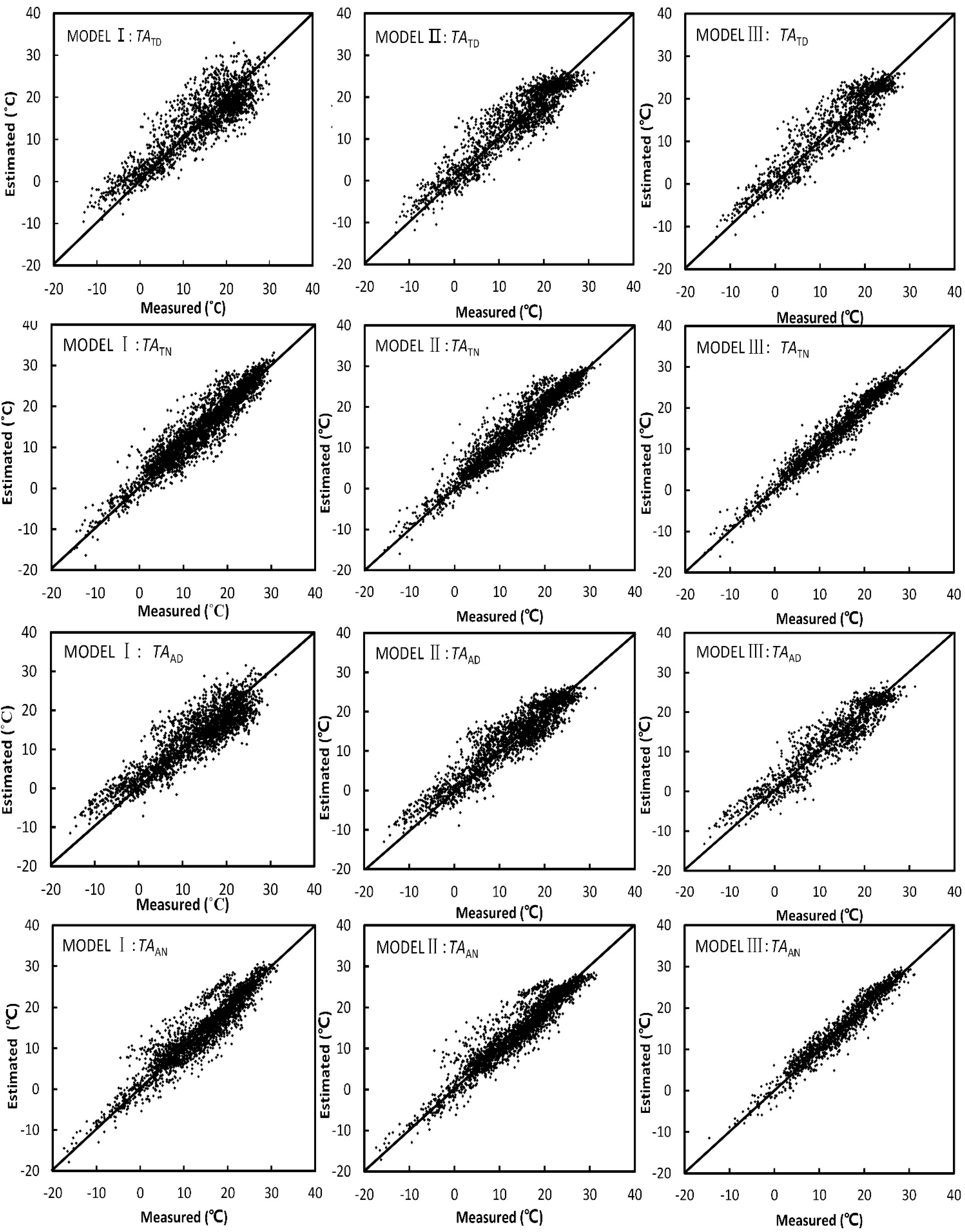
We generated the estimation models for daily mean air temperature based on the year-round LST data (Model I), the seasonal LST data (Model II), and the seasonal LST data for rural areas (Model III).

3.1. Calibration and Validation of the Estimation Models Using MODIS LSTs

3.1.1. Model I: The Estimation Models of Daily Mean Air Temperature Using Year-Round LST Data

Figure 2 shows the relationships between daily mean air temperatures (TA) based on data from all meteorological stations and the LSTs derived from the TERRA and AQUA MODIS products. The results show that TA was lower than daytime LST but higher than nighttime LST derived from both satellites. This is because the land surface is the source of heat for air near the surface, and absorbs solar radiation during the daytime and releases that heat at night through long-wave radiation. Differences between TA and LST would be accentuated by heat absorption during the insolation period. Therefore, the differences between TA and LST derived from AQUA MODIS (with an overpass at 1:50 PM local time) are greater than those derived from TERRA MODIS (with an overpass at 10:50 AM local time) during the daytime.

Figure 2. The relationship between observed TA at the 23 meteorological stations and the daytime and nighttime MODIS LSTs (2003 to 2011). The diagonal line from the origin represents the relationship TA = LST; the shorter lines represent the linear regression lines.

Figure 2. The relationship between observed TA at the 23 meteorological stations and the daytime and nighttime MODIS LSTs (2003 to 2011). The diagonal line from the origin represents the relationship TA = LST; the shorter lines represent the linear regression lines.

Figure 2 also shows a clear linear relationship between TA and the MODIS LSTs. Therefore, we used linear regression to establish the estimation models for TA as a function of the MODIS LST. The model fit was good (R² > 0.77, p < 0.001), with low errors (RMSE < 4.2 and biases < 0.001) for all models. When nighttime LSTs were used as estimators instead of daytime LSTs, the R² improved to values greater than 0.86. This means that LST_TD or LST_AD can explain at least 77% of the variance in TA, whereas LST_TN or LST_AN can explain at least 86% of the variance. In addition, the RMSEs for the regression equations based on nighttime LSTs as estimators were at least 20% smaller than those using daytime LSTs as estimators. This means that the night-time LSTs are better estimators of TA than the daytime LSTs. These results are consistent with other studies conducted in various regions [6,10,41].

There were differences between the AQUA and TERRA night point clouds. These point clouds are from measured and estimated data at the Huashan station. Huashan, located about 120 km east of Xi’an, is one of China’s Five Great Mountains. The highest point is the South Peak (Huashan station) at 2154.9 m. The complicated interlinks between ambient TA and LST can be explained by the balance between incoming shortwave radiation, incoming and outgoing long wave radiation, the surface albedo, the ground heat flux, and the sensible and latent heat fluxes. As a general rule, the land surface cools rapidly during the night to yield a negative LST−TA difference, and the longer after sunset, the bigger the difference. Therefore, the intercept of the equation between TA and LST_AN (7.3256) is greater than the intercept of the equation for the relationship between TA and LST_TN (5.5517) because the average overpass time for AQUA at night (1:50 AM) is later than that of TERRA at night (10:50 PM) for our study area. This is similar to the results of Shamir and Georgakakos’ [8]. However, TA is lower at the Huashan station because atmospheric temperature decreases with increasing altitude. Thus, the scatter plot between TA and LST_AN at Huashan station differs from that at the other stations and is closer to the line for TA = LST_AN. Therefore, LST_TN is a better predictor of TA than LST_AN in this context.

3.1.2. Model II: Estimation of Daily Mean Air Temperature Using Seasonal LST Data

Table 2 presents the linear regression equations for the relationship between TA and LST based on separate data for the spring, summer, fall, and winter. As in the case of Model I, all models were statistically significant (p < 0.001), but the nighttime LSTs were better estimators of TA than the daytime LSTs. The biases for all models were less than 0.04. We found that the RMSE values for the model estimates during the summer were equivalent to or slightly better than those in the other seasons. RMSE ≤ 2.7 for the summer estimation models, versus RMSEs ≤ 4.4, 3.2, and 3.1 for models in the spring, fall, and winter, respectively. The lowest R² and RMSE occurred during the summer. However, the diurnal temperature variation differs between the land surface and the air above it.

Compared with the RMSEs of estimation models based on year-round data (i.e., Model I), using seasonal LST_TD, LST_TN, LST_AD, and LST_AN as the independent variables (Figure 2) improved the model’s performance greatly in the summer, fall, and winter (Table 2). The RMSE of the estimation model for TA was 4.2 when year-round LST_TD was used as estimator, versus 2.6, 3.2, and 3.0, respectively, for the summer, fall, and winter models. The corresponding RMSEs for the LST_TN model were 1.9 (summer), 1.9 (fall), and 2.2 (winter), and were less than the RMSE for the year-round data (2.5) The RMSE for the model based on year-round LST_AD was 4.2 and was greater than those of the models for summer (2.6), fall (3.2), and winter (3.1). With the LST_AN models, the RMSEs for models in the summer (2.7), fall (2.8), and winter (2.7) were less than the RMSE (3.3) with the year-round data. The models for spring had estimation power similar to that of the models using the year-round data.

3.1.3. Model III: Estimation of Daily Mean Air Temperature for Agricultural Regions Using Seasonal LST Data

In the past few decades, with the accelerating rate of urbanization in China, the increasing amount of buildings, public squares, and roads in Shaanxi Province has decreased the amount of green space, water, and other natural surfaces. The surface thermodynamic properties differ greatly between urban and rural land. Buildings and artificial pavement represent the dominant urban surface, and because their materials have a high thermal conductivity, they absorb more of the incident solar radiation. This can cause greater atmospheric warming than would occur over natural surfaces such as vegetation, creating what is known as the “urban heat island” effect. As a result of urbanization, the urban temperature has therefore risen steadily [39]. In summer, when the surface temperature of grass lawns is 32 °C, cement roads may have a surface temperature of up to 57 °C, and asphalt surface temperatures may rise as high as 63 °C [42]. These high-temperature surfaces become a huge heat source for the surrounding atmosphere. High concentrations of air pollutants and increasing levels of aerosol particles also retain this heat by acting to some extent as insulators that trap outgoing radiation [43]. Kawashima et al. [44] pointed out that LSTs generally determine the variations of the surrounding air temperature. Therefore, the relationship between TA and LST derived from satellite data for urban environments will be quite different from that in rural regions. To enhance the estimation accuracy of TA for rural areas, we repeated our analysis after excluding data from urban stations and mountainous area.

Table 2. Estimation models for daily mean air temperature (TA) in the spring, summer, fall, and winter using the MODIS-derived land surface temperatures (LSTs) as the independent variable.

Independent Variable	Season	Model II	R2	RMSE	bias	N
LSTTD	Spring	TATD = 0. 529LSTTD + 1.185	0.4390	4.4	0.0002	3698
	Summer	TATD = 0.232LSTTD + 15.73	0.2280	2.6	0.0237	3007
	Fall	TATD = 0.8149LSTTD − 4.5194	0.7487	3.2	0.0168	3256
	Winter	TATD = 0.8542LSTTD − 6.0169	0.6620	3.0	0.0007	1589
LSTTN	Spring	TATN = 0.8626LSTTN + 7.7517	0.8241	2.5	0.0051	4213
	Summer	TATN =0.7113LSTTN + 10.503	0.6355	1.9	0.0082	3525
	Fall	TATN = 0.9039LSTTN + 4.7326	0.9015	1.9	0.0071	3654
	Winter	TATN = 0.8714LSTTN + 4.0055	0.879	2.2	−0.0011	2073
LSTAD	Spring	TAAD = 0.512LSTAD − 0.044	0.4070	4.2	0.0169	3473
	Summer	TAAD = 0.239LSTAD +14.86	0.2530	2.6	0.0338	2545
	Fall	TAAD = 0.784LSTAD − 6.012	0.7370	3.2	0.0180	3186
	Winter	TAAD = 0.716LSTAD − 7.752	0.6400	3.1	0.0048	1570
LSTAN	Spring	TAAN = 0.801LSTAN + 9.198	0.6710	3.3	0.0014	4095
	Summer	TAAN = 0.567LSTAN + 13.57	0.3941	2.7	0.0130	2971
	Fall	TAAN = 0.817LSTAN + 6.532	0.7620	2.8	0.0041	3134
	Winter	TAAN = 0.795LSTAN + 4.924	0.8250	2.7	−0.0057	1553

Table 2. Estimation models for daily mean air temperature (TA) in the spring, summer, fall, and winter using the MODIS-derived land surface temperatures (LSTs) as the independent variable.

Independent Variable	Season	Model II	R2	RMSE	bias	N
LSTTD	Spring	TATD = 0. 529LSTTD + 1.185	0.4390	4.4	0.0002	3698
	Summer	TATD = 0.232LSTTD + 15.73	0.2280	2.6	0.0237	3007
	Fall	TATD = 0.8149LSTTD − 4.5194	0.7487	3.2	0.0168	3256
	Winter	TATD = 0.8542LSTTD − 6.0169	0.6620	3.0	0.0007	1589
LSTTN	Spring	TATN = 0.8626LSTTN + 7.7517	0.8241	2.5	0.0051	4213
	Summer	TATN =0.7113LSTTN + 10.503	0.6355	1.9	0.0082	3525
	Fall	TATN = 0.9039LSTTN + 4.7326	0.9015	1.9	0.0071	3654
	Winter	TATN = 0.8714LSTTN + 4.0055	0.879	2.2	−0.0011	2073
LSTAD	Spring	TAAD = 0.512LSTAD − 0.044	0.4070	4.2	0.0169	3473
	Summer	TAAD = 0.239LSTAD +14.86	0.2530	2.6	0.0338	2545
	Fall	TAAD = 0.784LSTAD − 6.012	0.7370	3.2	0.0180	3186
	Winter	TAAD = 0.716LSTAD − 7.752	0.6400	3.1	0.0048	1570
LSTAN	Spring	TAAN = 0.801LSTAN + 9.198	0.6710	3.3	0.0014	4095
	Summer	TAAN = 0.567LSTAN + 13.57	0.3941	2.7	0.0130	2971
	Fall	TAAN = 0.817LSTAN + 6.532	0.7620	2.8	0.0041	3134
	Winter	TAAN = 0.795LSTAN + 4.924	0.8250	2.7	−0.0057	1553

Table 3 presents the TA estimation models based on the data from meteorological stations in rural regions in each season and the corresponding LSTs. There was generally a strong and statistically significant positive linear relationship between TA and the LSTs derived from the TERRA or AQUA MODIS products during both the daytime and nighttime. Estimates of TA improved (lower RMSE; Model III in Table 3) compared to those that included data from urban areas (Model II in Table 2) when using LST_AN or LST_AD as the independent variable. The RMSEs of Model III with LST_AN as the estimator were 2.3 (spring), 1.9 (summer), 1.9 (fall), and 2.3 (winter), which were less than the corresponding values of 3.3 (spring), 2.7 (summer), 2.8 (fall), and 2.7 (winter) for Model II. The RMSEs of Model III using LST_AD as the estimator were 4.0 (spring), 2.4 (summer), 3.0 (fall), and 3.0 (winter), versus RMSEs of 4.2 (spring), 2.6 (summer), 3.2 (fall), and 3.1 (winter) with Model II. With LST_TD or LST_TN as the estimator, Model III produced results similar to Model II. The RMSEs of Model III using LST_TN as the estimator were 2.5 (spring), 1.9 (summer), 1.7 (fall), and 2.2 (winter), versus 2.5 (spring), 1.9 (summer), 1.9 (fall), and 2.2 (winter) using Model II. The RMSEs of Model III using LST_TD as the estimator were 4.2 (spring), 2.7 (summer), 3.4 (fall), and 2.9 (winter), versus RMSEs of 4.4 (spring), 2.6 (summer), 3.2 (fall), and 3.0 (winter) using Model II.

Table 3. The seasonal estimation models for daily mean air temperature (TA) based on the corresponding land surface temperature (LST) data from meteorological stations in rural regions (i.e., Model III).

Independent Variable	Season	Model III	R2	RMSE	bias	N
LSTTD	Spring	TATD= 0.602LSTTD − 0.223	0.4860	4.2	0.0184	2460
	Summer	TATD = 0.238LSTTD + 15.52	0.2370	2.7	0.0260	2426
	Fall	TATD = 0.801LSTTD − 4.224	0.7250	3.4	0.0010	2657
	Winter	TATD = 0.844LSTTD − 5.819	0.6770	2.9	0.0047	1360
LSTTN	Spring	TATN = 0.864LSTTN + 7.772	0.8249	2.5	0.0002	3300
	Summer	TATN = 0.7215LSTTN + 10.279	0.6317	1.9	0.0195	2811
	Fall	TATN = 0.9223LSTTN + 4.5128	0.9140	1.7	0.0032	2869
	Winter	TATN = 0.8868LSTTN + 4.1513	0.8744	2.2	−0.0032	1575
LSTAD	Spring	TA AD = 0.519LSTAD − 0.134	0.4560	4.0	0.0099	2253
	Summer	TA AD = 0.249LSTAD + 14.50	0.2330	2.4	0.0307	1656
	Fall	TA AD = 0.848LSTAD − 6.987	0.7650	3.0	0.0057	2107
	Winter	TA AD = 0.737LSTAD − 7.824	0.6430	3.0	0.0011	1304
LSTAN	Spring	TAAN = 0.886LSTAN + 9.105	0.8120	2.3	0.0024	2412
	Summer	TAAN = 0.666LSTAN + 12.29	0.6520	1.9	0.0086	1926
	Fall	TAAN = 0.918LSTAN + 6.228	0.8770	1.9	0.0019	1908
	Winter	TAAN = 0.865LSTAN + 5.610	0.8760	2.3	−0.0049	810

Table 3. The seasonal estimation models for daily mean air temperature (TA) based on the corresponding land surface temperature (LST) data from meteorological stations in rural regions (i.e., Model III).

Independent Variable	Season	Model III	R2	RMSE	bias	N
LSTTD	Spring	TATD= 0.602LSTTD − 0.223	0.4860	4.2	0.0184	2460
	Summer	TATD = 0.238LSTTD + 15.52	0.2370	2.7	0.0260	2426
	Fall	TATD = 0.801LSTTD − 4.224	0.7250	3.4	0.0010	2657
	Winter	TATD = 0.844LSTTD − 5.819	0.6770	2.9	0.0047	1360
LSTTN	Spring	TATN = 0.864LSTTN + 7.772	0.8249	2.5	0.0002	3300
	Summer	TATN = 0.7215LSTTN + 10.279	0.6317	1.9	0.0195	2811
	Fall	TATN = 0.9223LSTTN + 4.5128	0.9140	1.7	0.0032	2869
	Winter	TATN = 0.8868LSTTN + 4.1513	0.8744	2.2	−0.0032	1575
LSTAD	Spring	TA AD = 0.519LSTAD − 0.134	0.4560	4.0	0.0099	2253
	Summer	TA AD = 0.249LSTAD + 14.50	0.2330	2.4	0.0307	1656
	Fall	TA AD = 0.848LSTAD − 6.987	0.7650	3.0	0.0057	2107
	Winter	TA AD = 0.737LSTAD − 7.824	0.6430	3.0	0.0011	1304
LSTAN	Spring	TAAN = 0.886LSTAN + 9.105	0.8120	2.3	0.0024	2412
	Summer	TAAN = 0.666LSTAN + 12.29	0.6520	1.9	0.0086	1926
	Fall	TAAN = 0.918LSTAN + 6.228	0.8770	1.9	0.0019	1908
	Winter	TAAN = 0.865LSTAN + 5.610	0.8760	2.3	−0.0049	810

3.1.4. Validation of the Estimation Models for Daily Mean Air Temperature

We validated the estimation models for TA using data from 2012 and 2013 at all available meteorological stations for models I and II, and data only from rural meteorological stations for model III. Figure 3 shows the relationship between the TA estimated using Model I, Model II, and Model III with the MODIS daytime and nighttime LSTs as independent variables and the TA measured at the meteorological stations. Most of the points were distributed around the line TA = LST. This indicates a good agreement between the estimated and measured TA. Model III tended to be more accurate than models I and II (Table 4).

Table 4 shows that Model III performed best. Model III generally had the highest coefficient of determination and lowest RMSE and MAE, or values comparable to those in the other models. Pairwise tests showed that the TA values estimated by Model III differed significantly (p < 0.01) from those estimated using Model I when LST_TD, LST_AD, or LST_AN was used as the estimator, but not for the model with LST_TN as the estimator (Table 5). The TA estimated by Model III differed significantly from that of Model II when LST_AD and LST_AN were used as the estimator (p < 0.05); for the TERRA datasets, the difference was not significant. In addition, Model II differed significantly from Model I (p < 0.01) only when the daytime LST data were used.

Figure 3. Relationships between the estimated and measured daily mean air temperature (TA) based on daytime (D) and nighttime (N) data for the three models (I = all data, II = seasonal data, III = seasonal data from rural stations). Table 4 provides statistical data on the results of each linear regression.

Figure 3. Relationships between the estimated and measured daily mean air temperature (TA) based on daytime (D) and nighttime (N) data for the three models (I = all data, II = seasonal data, III = seasonal data from rural stations). Table 4 provides statistical data on the results of each linear regression.

Table 4. Validation of the estimated daily mean air temperature (TA) predicted using land surface temperature (LST) data from meteorological stations for the three models in 2012 and 2013.

Independent	MODEL I				MODEL II				MODEL III
Variable	R2	RMSE	MAE	Bias	R2	RMSE	MAE	Bias	R2	RMSE	MAE	Bias
LSTTD	0.7791	4.3	3.38	0.2345	0.8622	3.4	2.66	−0.3462	0.867	3.4	2.7	0.4096
LSTTN	0.8941	2.9	2.20	0.7119	0.9176	2.6	1.87	−0.7445	0.9516	2.0	1.56	−0.6007
LSTAD	0.795	4.1	3.27	−0.1203	0.8649	3.3	2.62	0.2830	0.887	3.2	2.52	0.3737
LSTAN	0.8633	3.2	2.32	0.2886	0.8919	2.8	2.01	0.2572	0.94	2.0	1.54	0.3467

Table 4. Validation of the estimated daily mean air temperature (TA) predicted using land surface temperature (LST) data from meteorological stations for the three models in 2012 and 2013.

Independent	MODEL I				MODEL II				MODEL III
Variable	R2	RMSE	MAE	Bias	R2	RMSE	MAE	Bias	R2	RMSE	MAE	Bias
LSTTD	0.7791	4.3	3.38	0.2345	0.8622	3.4	2.66	−0.3462	0.867	3.4	2.7	0.4096
LSTTN	0.8941	2.9	2.20	0.7119	0.9176	2.6	1.87	−0.7445	0.9516	2.0	1.56	−0.6007
LSTAD	0.795	4.1	3.27	−0.1203	0.8649	3.3	2.62	0.2830	0.887	3.2	2.52	0.3737
LSTAN	0.8633	3.2	2.32	0.2886	0.8919	2.8	2.01	0.2572	0.94	2.0	1.54	0.3467

Table 5. Significant test between the different estimation values of daily mean air temperature using the three model types with the MODIS LSTs as the predictor.

	Pairwise Test Result (p level)
	Model III/Model I	Model III/Model II	Model II/Model I
LSTTD	0.0000	0.0933	0.0022
LSTTN	0.1795	0.0513	0.2021
LSTAD	0.0000	0.0106	0.0001
LSTAN	0.0093	0.0109	0.4708

Table 5. Significant test between the different estimation values of daily mean air temperature using the three model types with the MODIS LSTs as the predictor.

	Pairwise Test Result (p level)
	Model III/Model I	Model III/Model II	Model II/Model I
LSTTD	0.0000	0.0933	0.0022
LSTTN	0.1795	0.0513	0.2021
LSTAD	0.0000	0.0106	0.0001
LSTAN	0.0093	0.0109	0.4708

3.2. Optimal Strategies for Merging Images of Daily Mean Air Temperature Estimated from LSTs

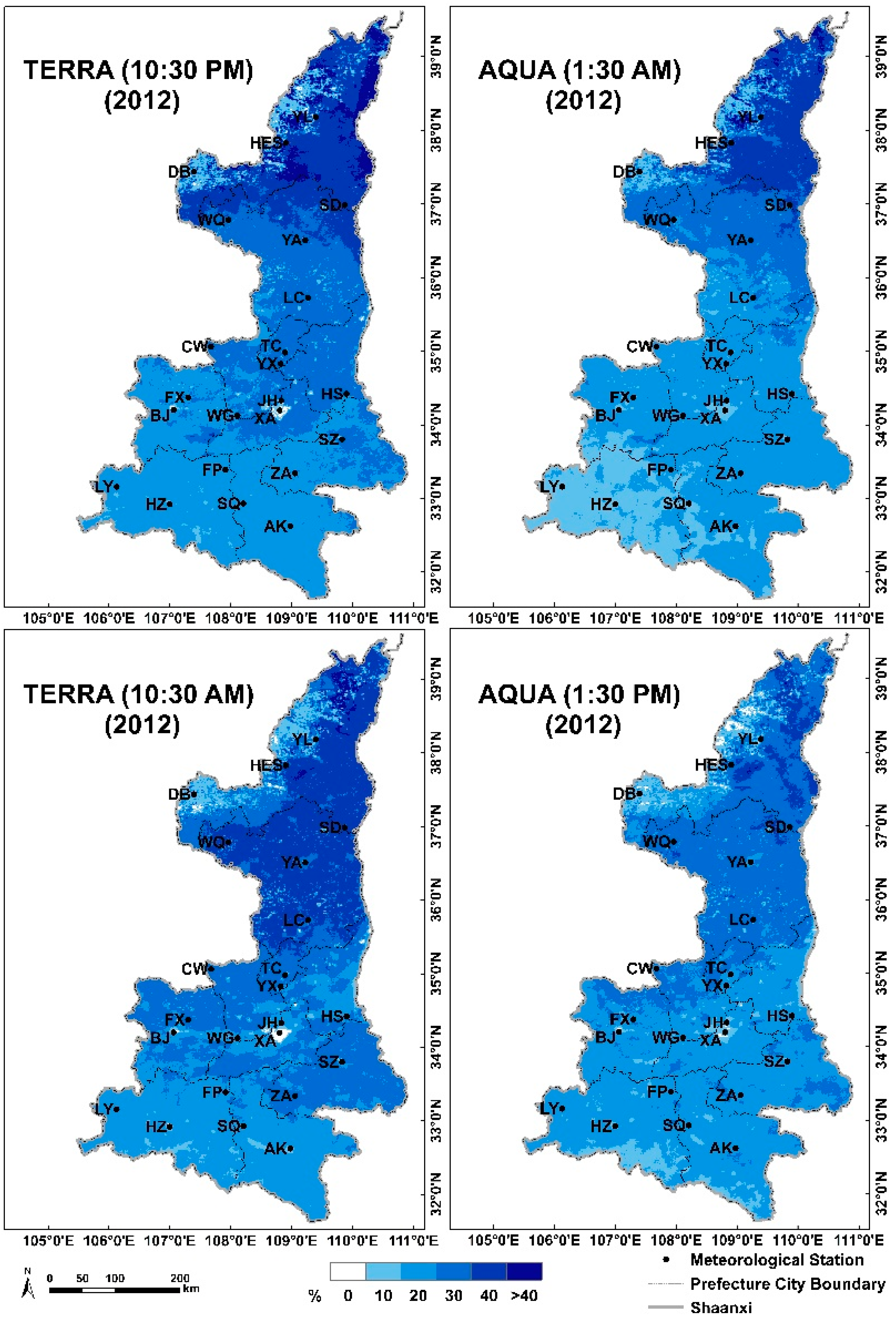
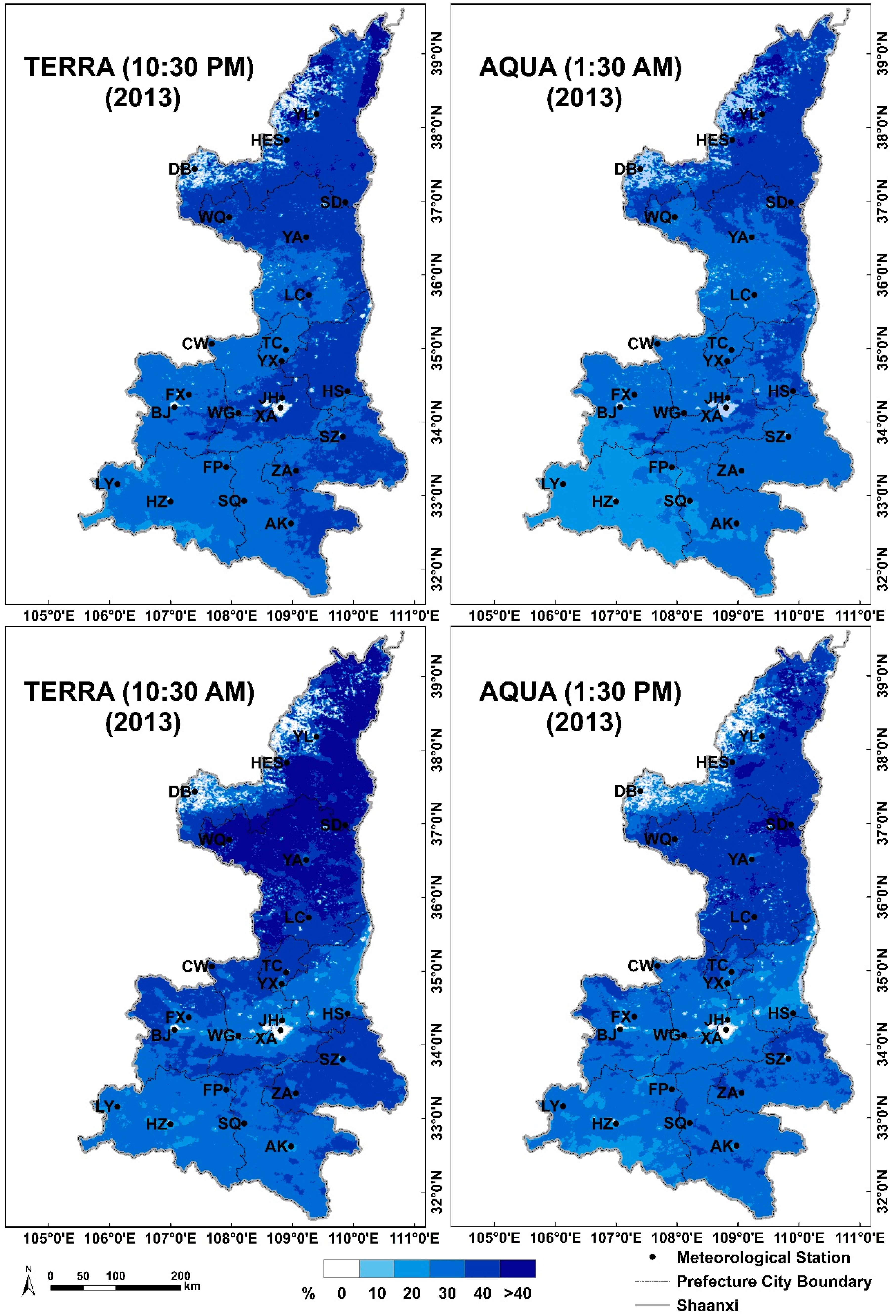
We created maps of TA values for each day from 2003 to 2013. We obtained a maximum of four TA images on each clear day (i.e., the daytime and nighttime LSTs from the TERRA and AQUA MODIS products). However, because of cloud cover, one or more of these datasets was often unavailable for certain parts of the study area, and the resulting map of estimated TA suffered from gaps. Figure 4 and Figure 5 present the proportion of the data available for each pixel in the study area based on the daytime and nighttime TERRA and AQUA MODIS LSTs in 2012 and 2013, respectively. Most of the pixels in the study area had availability values of less than 50%. 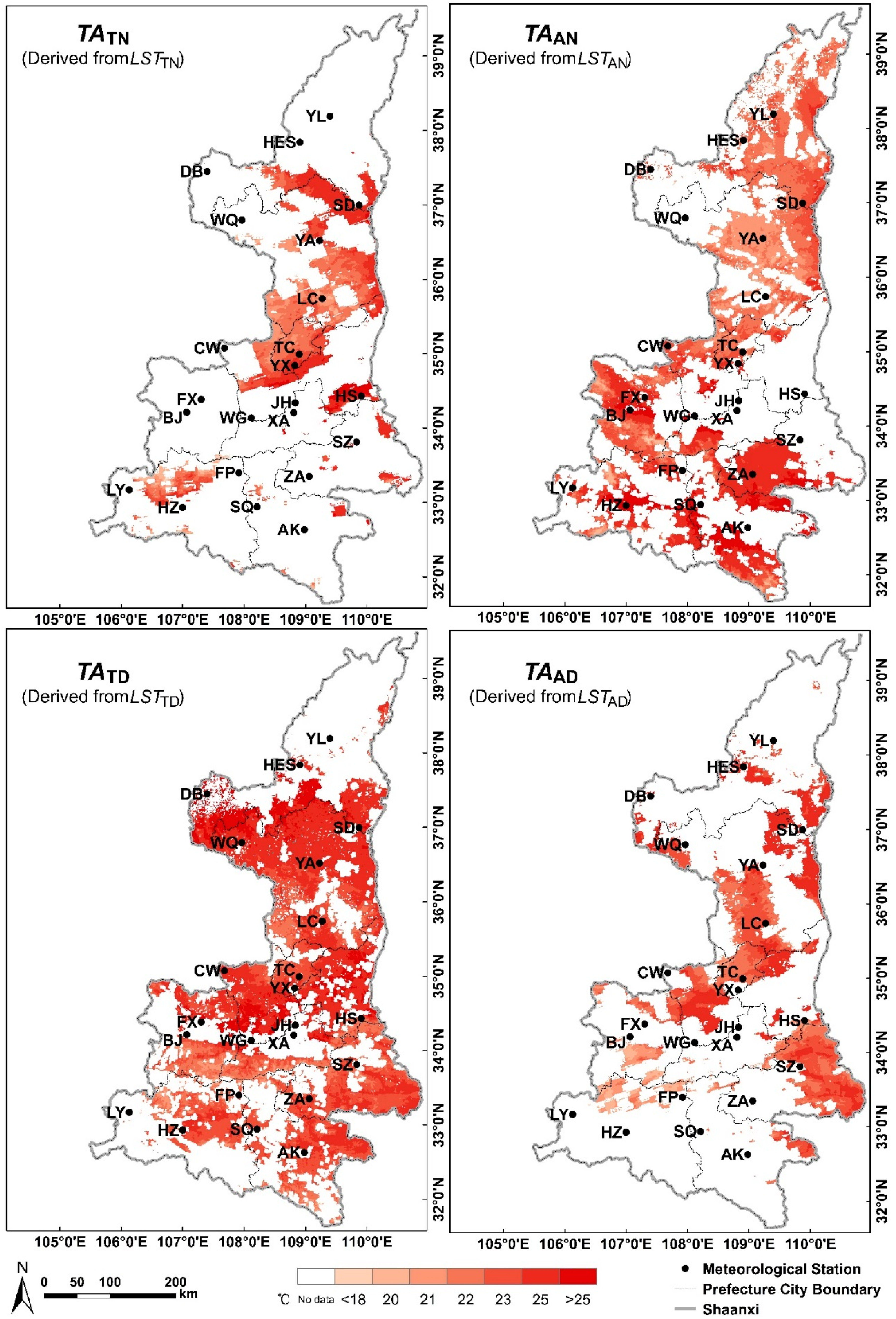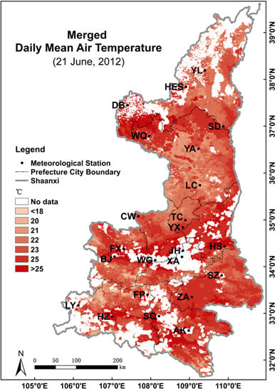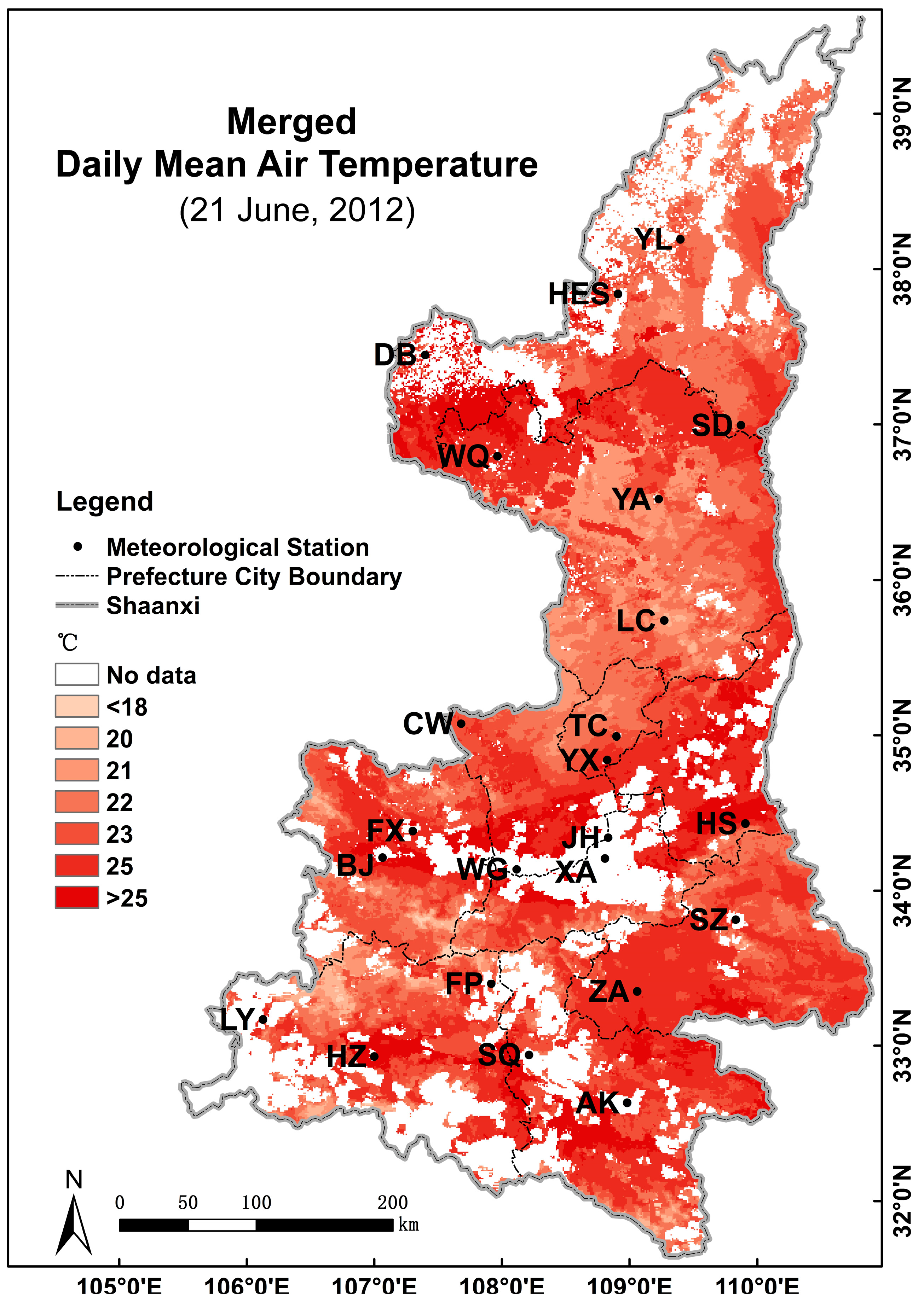For example, Figure 6 shows that on 21 June 2012, the available data amounted to only 18.40, 40.81, 51.04, and 24.29% of the pixels for TA_TN, TA_AN, TA_TD, and TA_AD, respectively. Fortunately, the available data from the different MODIS products both overlap and complement each other, which makes it possible to merge the data to increase data availability for the study area. Figure 7 provides examples of merged TA data for 21 June 2012. The available data coverage in the merged image totaled 75.58%, which represents an increase of 57.18, 34.77, 24.54, and 51.29 percentage points compared with the coverage based only on TA_TN, TA_AN, TA_TD, and TA_AD, respectively.

Table 4 shows that the RMSEs using Model III were 3.4, 2.0, 3.2, and 2.0 when using LST_TD, LST_TN, LST_AD, and LST_AN as the estimator, respectively, and the corresponding MAEs were 2.70, 1.56, 2.52, and 1.54. This means that combining the different TA images calculated using the different LST products will result in a different accuracy. Table 6 shows the possible strategies for combining TA images. In strategy 1, for instance, the TA_TN image was the initial basis for the merged data. When the TA_TN value was missing, it was replaced by the TA_AN value. If both TA_TN and TA_AN were missing, they were replaced by the TA_AD value. When all three were missing, they were replaced by the TA_TD value. The values in Table 6 were calculated independently for each grid cell throughout the study area.

Figure 4. Percentages of available data for daily mean air temperature (TA) in 2012 based on daytime and nighttime TERRA and AQUA MODIS land surface temperatures (LSTs).

Figure 4. Percentages of available data for daily mean air temperature (TA) in 2012 based on daytime and nighttime TERRA and AQUA MODIS land surface temperatures (LSTs).

Figure 5. Percentages of available data for daily mean air temperature (TA) in 2013 based on daytime and nighttime TERRA and AQUA MODIS land surface temperatures (LSTs).

Figure 5. Percentages of available data for daily mean air temperature (TA) in 2013 based on daytime and nighttime TERRA and AQUA MODIS land surface temperatures (LSTs).

Figure 6. Daily mean air temperature (TA) estimated using the daytime and nighttime land surface temperatures (LSTs) from the TERRA and AQUA MODIS products for 21 June 2012.

Figure 6. Daily mean air temperature (TA) estimated using the daytime and nighttime land surface temperatures (LSTs) from the TERRA and AQUA MODIS products for 21 June 2012.

Figure 7. Merged image using the daily mean air temperatures (TAs) estimated using the daytime and nighttime land surface temperatures (LSTs) from the TERRA and AQUA MODIS products for 21 June 2012.

Figure 7. Merged image using the daily mean air temperatures (TAs) estimated using the daytime and nighttime land surface temperatures (LSTs) from the TERRA and AQUA MODIS products for 21 June 2012.

Based on results in Table 6, we found that R² varies between 0.9073 and 0.9383, the RMSEs range from 2.41 to 2.91, MAE change from 1.84 to 2.24, and bias varies between −0.5049 and −0.3421. The merged results had a higher R² and a lower RMSE and MAE if TA_TN and TA_AN were used as the first two merged images (strategies 1, 2, 7, and 8). The prediction ability was high in each case, with R² > 0.93, RMSE ≤ 2.43, and MAE ≤ 1.87 in all cases. In contrast, if we used TA_TD and TA_AD as the first two merged images (strategies 17, 18, 23, and 24), R² decreased (to values <0.92) and RMSE and MAE increased (to values ≥ 2.76 and 2.11, respectively). 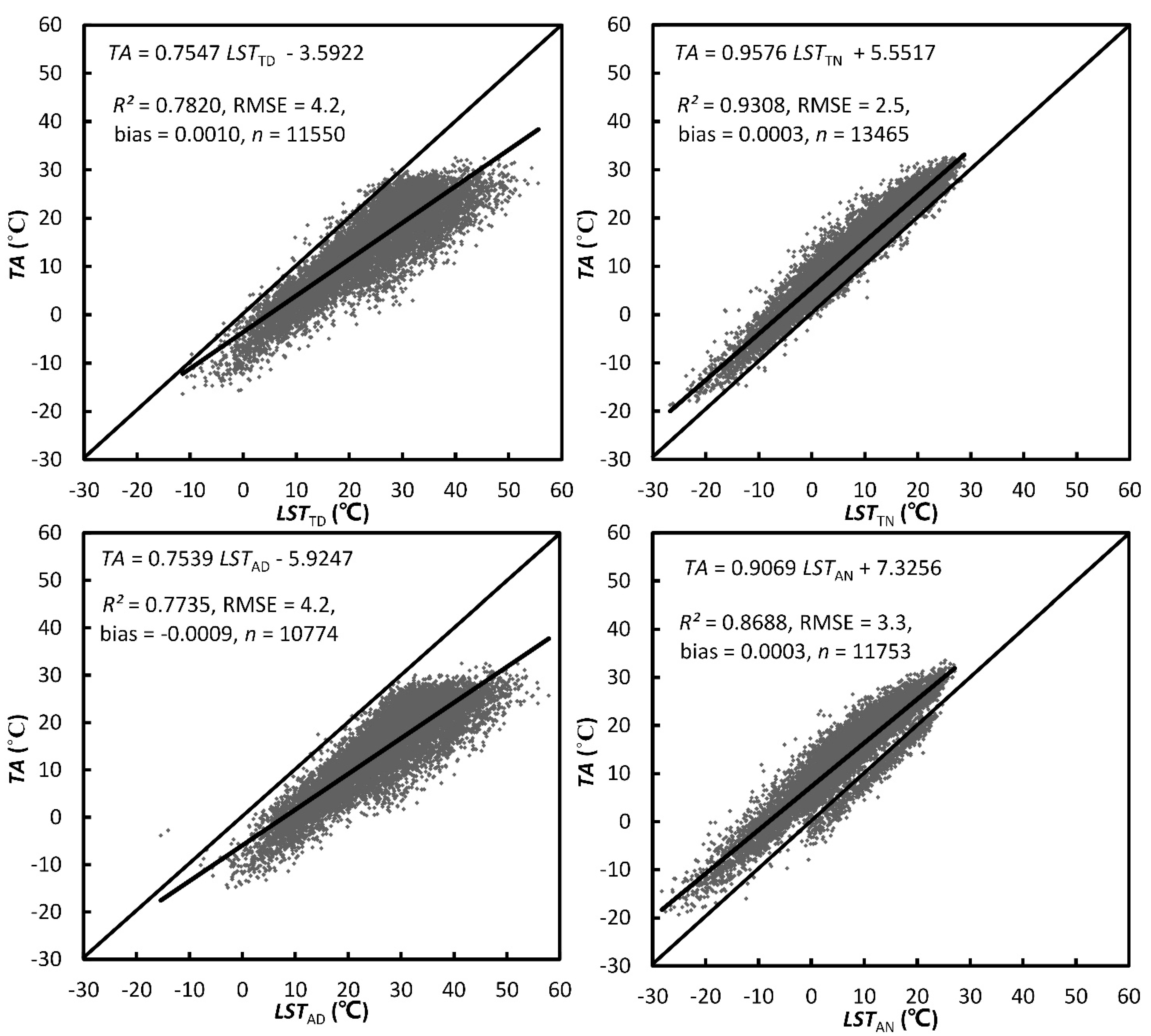This is because the R² between TA and nighttime LSTs was stronger than those between TA and daytime LSTs (Section 3.1). The estimation models based on nighttime LSTs had lower RMSEs and MAEs. The optimal combination of TA images was provided by Strategy 2; although Strategy 18 produced similar results, the R² value was higher for Strategy 2. Therefore, we chose Strategy 2 as the optimal combination of the four TA images.

Table 6. Possible image merging strategies to create maps of daily mean air temperature (TA) using the TERRA and AQUA MODIS land surface temperatures (LSTs) and their accuracy using the validation datasets from 2012 to 2013.

Strategy	Base Image	Second Image	Third Image	Fourth Image	R2	RMSE	MAE	bias
1	TATN	TAAN	TAAD	TATD	0.9381	2.42	1.84	−0.4549
2	TATN	TAAN	TATD	TAAD	0.9383	2.41	1.84	−0.4190
3	TATN	TAAD	TAAN	TATD	0.9352	2.48	1.90	−0.5033
4	TATN	TAAD	TATD	TAAN	0.9338	2.51	1.92	−0.5049
5	TATN	TATD	TAAN	TAAD	0.9361	2.45	1.87	−0.4215
6	TATN	TATD	TAAD	TAAN	0.9341	2.49	1.91	−0.4541
7	TAAN	TATN	TAAD	TATD	0.9367	2.43	1.87	−0.4501
8	TAAN	TATN	TATD	TAAD	0.9369	2.42	1.87	−0.4141
9	TAAN	TAAD	TATN	TATD	0.9299	2.54	1.94	−0.3851
10	TAAN	TAAD	TATD	TATN	0.9253	2.63	2.00	−0.4348
11	TAAN	TATD	TATN	TAAD	0.9281	2.57	1.96	−0.4073
12	TAAN	TATD	TAAD	TATN	0.9250	2.62	2.00	−0.3756
13	TAAD	TAAN	TATN	TATD	0.9170	2.76	2.13	−0.4245
14	TAAD	TAAN	TATD	TATN	0.9124	2.84	2.19	−0.4743
15	TAAD	TATN	TAAN	TATD	0.9190	2.74	2.10	−0.4443
16	TAAD	TATN	TATD	TAAN	0.9124	2.84	2.19	−0.4743
17	TAAD	TATD	TATN	TAAN	0.9097	2.89	2.22	−0.4794
18	TAAD	TATD	TAAN	TATN	0.9079	2.91	2.24	−0.4647
19	TATD	TAAN	TATN	TAAD	0.9167	2.76	2.11	−0.3739
20	TATD	TAAN	TAAD	TATN	0.9136	2.81	2.15	−0.3421
21	TATD	TATN	TAAN	TAAD	0.9183	2.74	2.09	−0.3769
22	TATD	TATN	TAAD	TAAN	0.9162	2.78	2.13	−0.4095
23	TATD	TAAD	TAAN	TATN	0.9073	2.91	2.24	−0.3562
24	TATD	TAAD	TATN	TAAN	0.9091	2.89	2.22	−0.3709

Table 6. Possible image merging strategies to create maps of daily mean air temperature (TA) using the TERRA and AQUA MODIS land surface temperatures (LSTs) and their accuracy using the validation datasets from 2012 to 2013.

Strategy	Base Image	Second Image	Third Image	Fourth Image	R2	RMSE	MAE	bias
1	TATN	TAAN	TAAD	TATD	0.9381	2.42	1.84	−0.4549
2	TATN	TAAN	TATD	TAAD	0.9383	2.41	1.84	−0.4190
3	TATN	TAAD	TAAN	TATD	0.9352	2.48	1.90	−0.5033
4	TATN	TAAD	TATD	TAAN	0.9338	2.51	1.92	−0.5049
5	TATN	TATD	TAAN	TAAD	0.9361	2.45	1.87	−0.4215
6	TATN	TATD	TAAD	TAAN	0.9341	2.49	1.91	−0.4541
7	TAAN	TATN	TAAD	TATD	0.9367	2.43	1.87	−0.4501
8	TAAN	TATN	TATD	TAAD	0.9369	2.42	1.87	−0.4141
9	TAAN	TAAD	TATN	TATD	0.9299	2.54	1.94	−0.3851
10	TAAN	TAAD	TATD	TATN	0.9253	2.63	2.00	−0.4348
11	TAAN	TATD	TATN	TAAD	0.9281	2.57	1.96	−0.4073
12	TAAN	TATD	TAAD	TATN	0.9250	2.62	2.00	−0.3756
13	TAAD	TAAN	TATN	TATD	0.9170	2.76	2.13	−0.4245
14	TAAD	TAAN	TATD	TATN	0.9124	2.84	2.19	−0.4743
15	TAAD	TATN	TAAN	TATD	0.9190	2.74	2.10	−0.4443
16	TAAD	TATN	TATD	TAAN	0.9124	2.84	2.19	−0.4743
17	TAAD	TATD	TATN	TAAN	0.9097	2.89	2.22	−0.4794
18	TAAD	TATD	TAAN	TATN	0.9079	2.91	2.24	−0.4647
19	TATD	TAAN	TATN	TAAD	0.9167	2.76	2.11	−0.3739
20	TATD	TAAN	TAAD	TATN	0.9136	2.81	2.15	−0.3421
21	TATD	TATN	TAAN	TAAD	0.9183	2.74	2.09	−0.3769
22	TATD	TATN	TAAD	TAAN	0.9162	2.78	2.13	−0.4095
23	TATD	TAAD	TAAN	TATN	0.9073	2.91	2.24	−0.3562
24	TATD	TAAD	TATN	TAAN	0.9091	2.89	2.22	−0.3709

The LSTs from MODIS TERRA and AQUA are retrieved only under clear-sky conditions. LSTs under cloudy conditions would differ from those obtained under a clear sky. In contrast, TA is available irrespective of cloud conditions. It is therefore important to analyze the influence of clouds on the estimation of TA. Table 7 summarizes the difference between the measured and estimated TA under four different cases of cloud conditions. In Case 1, pixels from all four datasets are cloud-free. In Case 2, pixels from three of the four datasets are cloud-free. In Case 3, pixels from two of the four datasets are cloud-free. In Case 4, pixels from only one of the four datasets are cloud-free. Case 5 means that pixels are contaminated with clouds in all four LST products, so LST is instead estimated by means of interpolation between adjacent pixels (we will describe the interpolation method in Section 3.3). In Case 2, Case 3 and Case 4, missing pixels due to cloudiness in different datasets were filled with corresponding cloud-free pixels in another dataset which means that TA could have been overestimated (i.e., because LST would be lower as a result of the shade created by clouds). In Case 5, missing pixels were interpolated from surrounding cloud-free pixels, leading to a positive bias. The bias also varied seasonally. In winter, as the vegetation coverage is lower, bare soil and built structures receive more solar radiation, which causes a slightly higher bias when daytime LST is merged into the map. In summer, vegetation and water reduce the temperature difference during the daytime and nighttime. The results show no obvious relationship among the four cases because the LSTs from the MODIS Terra and Aqua have already been filtered to eliminate cloud cover using the QC data. Under these circumstances, the data merging method proposed in this study has no consistent bias that must be adjusted to account for cloudiness.

Table 7. Bias between measured and estimated daily mean air temperature (TA) under different cloud conditions for the merged data from four MODIS datasets using data from 2012 and 2013. Cases: 1 = pixels from all four datasets are cloud-free; 2 = pixels from three of the four datasets are cloud-free; 3 = pixels from two of the four datasets are cloud-free; 4 = pixels from one of the four datasets are cloud-free; 5 = pixels are contaminated with clouds in all four datasets and must be estimated by means of interpolation of data from adjacent pixels.

Case	Whole Year	Spring	Summer	Autumn	Winter
1	−0.4837	−0.8475	−0.3088	−0.3207	−0.2039
2	−0.6341	−0.3766	−1.0319	−0.4779	−0.7821
3	−0.3775	−0.2540	−0.6404	−0.0127	−1.0149
4	−0.3979	−0.0953	−0.4046	−0.4798	−0.7197
5	0.0646	−0.1483	−0.1535	0.4003	0.3944

Table 7. Bias between measured and estimated daily mean air temperature (TA) under different cloud conditions for the merged data from four MODIS datasets using data from 2012 and 2013. Cases: 1 = pixels from all four datasets are cloud-free; 2 = pixels from three of the four datasets are cloud-free; 3 = pixels from two of the four datasets are cloud-free; 4 = pixels from one of the four datasets are cloud-free; 5 = pixels are contaminated with clouds in all four datasets and must be estimated by means of interpolation of data from adjacent pixels.

Case	Whole Year	Spring	Summer	Autumn	Winter
1	−0.4837	−0.8475	−0.3088	−0.3207	−0.2039
2	−0.6341	−0.3766	−1.0319	−0.4779	−0.7821
3	−0.3775	−0.2540	−0.6404	−0.0127	−1.0149
4	−0.3979	−0.0953	−0.4046	−0.4798	−0.7197
5	0.0646	−0.1483	−0.1535	0.4003	0.3944

3.3. Temporal and Spatial Fusion of Daily Mean Air Temperature Using Time Series Images

Figure 8 demonstrates the spatial distribution of data availability for each pixel using data for the whole year in 2012 and 2013. The merged image greatly improved the spatial coverage by the available data. Table 8 presents the annual data availability percentages for the TA images throughout the study area for the merged images and for images derived from daytime and nighttime TERRA and AQUA MODIS LSTs in 2012 and 2013. The results show that the merged image greatly improved the spatial coverage by the available data, reaching values of 55.46% in 2012 and 44.92% in 2013. But the percentages of available data were 22.08%, 17.94%, 22.48%, and 18.65% for TA_TN, TA_AN, TA_TD, and TA_AD images in 2012. They were 28.85%, 25.23%, 31.30%, and 27.84%, respectively, in 2013. The available data in the merged images therefore increased by 33.38, 37.52, 32.98, and 36.81 percentage points in 2012 and by 16.07, 19.69, 13.62, and 17.08 percentage points in 2013 compared with the corresponding TA_TN, TA_AN, TA_TD, and TA_AD images. However, given the fact that data for an average of half of the pixels were unavailable even after merging the images, it is clearly necessary to obtain fuller spatial coverage to improve the accuracy of estimation of TA.

Figure 8. Percentages of data availability for daily mean air temperature (TA) in 2012 and 2013 for merged images based on the validation dataset.

Figure 8. Percentages of data availability for daily mean air temperature (TA) in 2012 and 2013 for merged images based on the validation dataset.

Table 8. Percentages of the daily mean air temperature (TA) images for the merged dataset (all four MODIS LST products combined using strategy 2 in Table 6) and for images derived from daytime and nighttime TERRA and AQUA MODIS LSTs in 2012 and 2013.

		Data Availability (%for Coverage, Percentage Points for Increase)
Year	Merged coverage	TATN		TAAN		TATD		TAAD
		coverage	increase	coverage	increase	coverage	increase	coverage	increase
2012	55.46	22.08	33.38	17.94	37.52	22.48	32.98	18.65	36.81
2013	44.92	28.85	16.07	25.23	19.69	31.30	13.62	27.84	17.08

Table 8. Percentages of the daily mean air temperature (TA) images for the merged dataset (all four MODIS LST products combined using strategy 2 in Table 6) and for images derived from daytime and nighttime TERRA and AQUA MODIS LSTs in 2012 and 2013.

		Data Availability (%for Coverage, Percentage Points for Increase)
Year	Merged coverage	TATN		TAAN		TATD		TAAD
		coverage	increase	coverage	increase	coverage	increase	coverage	increase
2012	55.46	22.08	33.38	17.94	37.52	22.48	32.98	18.65	36.81
2013	44.92	28.85	16.07	25.23	19.69	31.30	13.62	27.84	17.08

Ideally, the TA for crop growth monitoring and model simulation should take advantage of complete datasets. In reality, noise and missing pixels create gaps in the data that must be filled somehow. Aiming to achieve improved accuracy of TA will require efforts to reduce the loss of data and fill gaps, thereby providing better coverage of the whole study region. The daily mean temperature images before the date of the estimation are obtained if their data are available. These images carry important information for the TA estimation for the present day. We therefore proposed a method to fill gaps in the data based on the assumption that atmospheric conditions would be uniform within a relatively small window surrounding a pixel for which data is missing. This means that the TA difference of a target pixel between data t and data t-1 is equal to the mean TA difference of surrounding pixels between data t and data t-1. To minimize the uncertainty in the error introduced by cloudiness and gaps between swaths, we exploited a possible strategy based on finding the optimal window size by extending the process into a larger geographic area. The optimum window size was obtained from statistical analysis of the difference between TA estimated from the MODIS LST and TA measured by the meteorological stations. 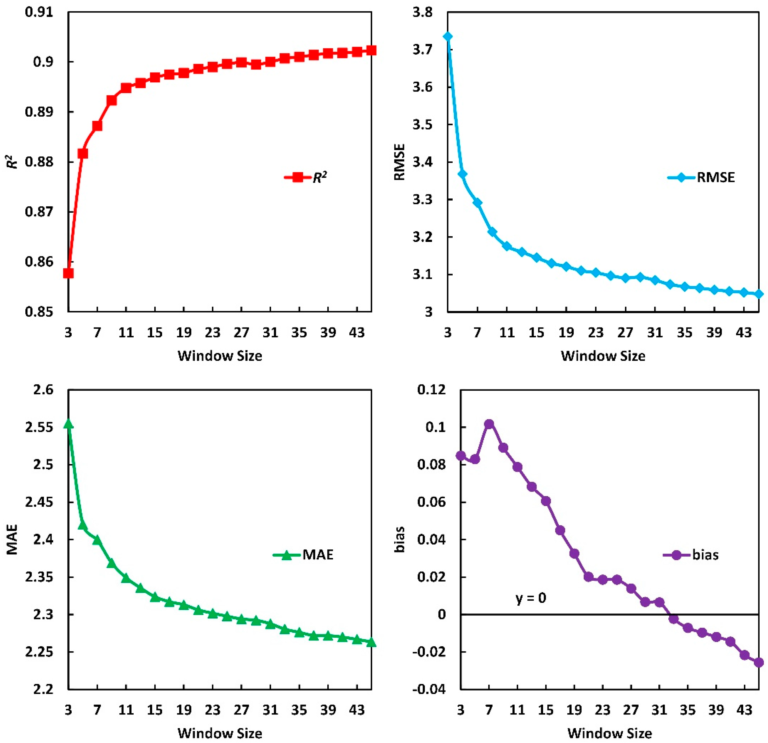Figure 9 displays the change in the quality of the estimate as a function of the window size used for the spatial filling. Figure 10 illustrates this estimation procedure (using a window size of 9 × 9 pixels as an example). The R² increased with increasing window size. In the contrast, RMSE, MAE, and bias decreased with increasing window size. The magnitude of the bias reached its minimum at a window size of 33 × 33 pixels. We therefore used a grid of 33 × 33 pixels centered on the pixel with missing data in our subsequent analysis. The mean difference in TA among these pixels is calculated as follows:

$$\overline{∆TA}=\frac{1}{\text{N}}{\displaystyle \sum }_{\text{j}=\text{i}-4}^{\text{j}+4}{\displaystyle \sum }_{\text{i}=\text{i}-4}^{\text{i}+4}\left(T{A}_{i, j}^t-T{A}_{i, j}^{t-1}\right)$$

(8)

where $\overline{∆TA}$ is the mean TA difference among the pixels with available data both at the date of estimation (i.e., at time t) and the date before the estimation (i.e., at time t–1). N is the number of pixels with available TA values both at the date of estimation and the date before estimation. $T{A}_{i, j}^t$ and $T{A}_{i, j}^{t-1}$ are the TA values for the pixel in line i and column j of the image at times t and t–1.

$T{A}_{i, j}^t$ can be estimated as follows:

$$T{A}_{i, j}^t=T{A}_{i, j}^{t-1}+\overline{∆TA}$$

(9)

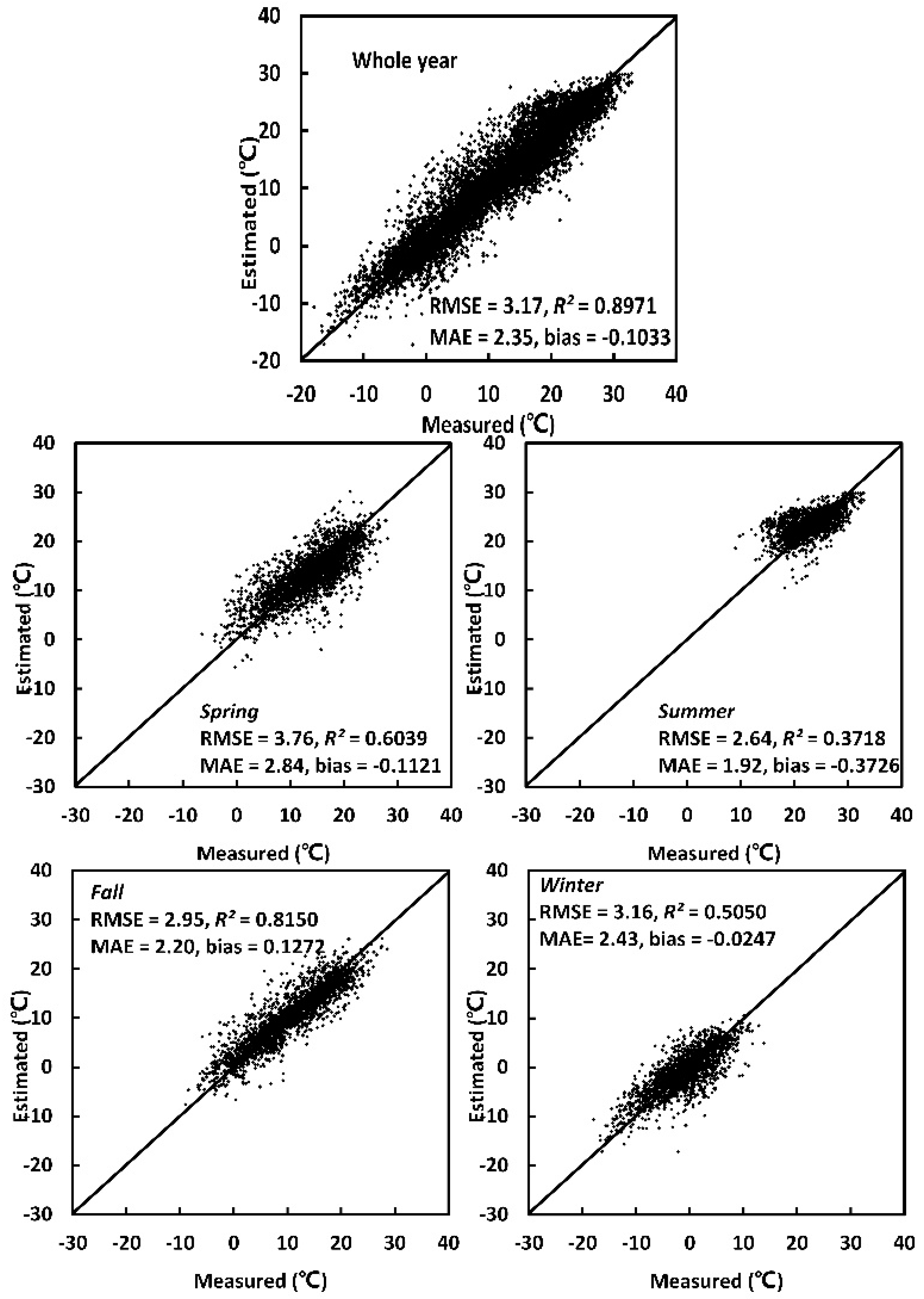
We used this approach to generate a time series of filled pixels using data for the whole year derived from the 14 rural meteorological stations in both 2012 and 2013. Figure 11 shows the resulting relationship between the estimated and measured TA. Overall, the approach produced good results: a strong and statistically significant relationship (R² = 0.8971) with a low MAE (2.35) for data from all seasons. Using the filled dataset increased data coverage to 78.23% and 86.02% in 2012 and 2013, respectively. The model showed a seasonal pattern of error. In summer, the R² was relatively poor and the distribution of the data was more concentrated than in other seasons which led to a lower RMSE. In turn, the higher LST increased turbulence in the atmospheric boundary layer, thereby affecting heat transfer from the land surface into the ambient air and subsequently to the upper atmosphere. In contrast, the land surface receives less solar radiation in winter, thereby weakening turbulence. The retrieval of TA is simpler at night because solar radiation does not affect the thermal infrared signal. Figure 12 demonstrates the day-to-day variation of the measured and estimated daily mean air temperature in 2012 and 2013 at the 14 rural meteorological stations. Judging from the similarity of the measured and estimated air temperatures (i.e., the difference was small and centered on 0 °C), the estimation model generally showed good agreement with the measured TA and was able to reflect the annual pattern of TA fluctuation. We found no systematically positive or negative biases between the estimated and measured values (Figure 11 and Figure 12).

Figure 9. Analysis the optimal size (pixels) of the window used for the spatial filling method illustrated in Figure 10.

Figure 9. Analysis the optimal size (pixels) of the window used for the spatial filling method illustrated in Figure 10.

Figure 10. Flowchart for calculation of missing pixel values caused by cloud cover and other problems using the merged images from the day before the estimation date The red square represents the pixel for which TA will be calculated based on data from the previous day.

Figure 10. Flowchart for calculation of missing pixel values caused by cloud cover and other problems using the merged images from the day before the estimation date The red square represents the pixel for which TA will be calculated based on data from the previous day.

Figure 11. Relationships between the estimated and measured daily mean air temperature (TA) for whole-year data and for data from the spring, summer, fall, and winter.

Figure 11. Relationships between the estimated and measured daily mean air temperature (TA) for whole-year data and for data from the spring, summer, fall, and winter.

Figure 12. Annual variation in the measured and estimated daily mean air temperature (TA) in 2012 and 2013 based on the data from the 14 rural meteorological stations.

Figure 12. Annual variation in the measured and estimated daily mean air temperature (TA) in 2012 and 2013 based on the data from the 14 rural meteorological stations.

4. Conclusions

If clouds are present at a given location, then LST data will not be available. In this paper, we describe a systematic method for filling such gaps in the data based on spatial and temporal data fusion techniques. The first step in this method was to find the optimal strategy for merging images of daily mean air temperature (TA) estimated from daytime and nighttime TERRA and AQUA LST data. The second step was to select the optimal spatial window size to use in interpolation and gap-filling based on estimated TA from the previous day. This process generates high spatial and temporal coverage for the study area. The calibration results showed that the annual average spatial coverage could be improved significantly. Using this approach, the proportion of the pixels with available data increases from 20.28% to 76.99% in 2012 and 28.31% to 89.67% in 2013.

The relationship between TA from the meteorological stations and LSTs derived from the daytime and nighttime TERRA and AQUA MODIS LST data was strong and significant. The nighttime LSTs from TERRA and AQUA MODIS provided a better TA estimator than the daytime LSTs. By comparing different strategies for merging the four TA images calculated using the daytime and nighttime TERRA and AQUA MODIS LST data in different orders, we found an optimal merging strategy (Table 6, Strategy 2). That is, TA_TN was used as the initial image, followed by the TA_AN value if the TA_TN value was missing; if both were missing, the TA_TD value was used, and if all three were missing, the TA_AD value was used. This strategy greatly increased the spatial coverage, and achieved the highest R² and lowest RMSE and MAE among the 24 possible merging strategies. Since this method depends on the availability of TERRA and AQUA daytime and nighttime data, it is of the greatest value under conditions of partial or short-lived cloud cover.

The validation results demonstrate that the data availability was only 55.46% in 2012 and 44.92% in 2013 after the first processing step. Therefore, more effort should be made to increase the spatial coverage of the available data. The relative proximity of air temperature difference between the estimated date and the previous days near the estimated pixels provides an opportunity to predict the missing data, most of which resulted from cloud contamination. The second step was to determine the difference in TA between the estimation date and previous days for every pixel within a selected window size. Adding the mean differences for these pixels to the value for the center pixel from the previous day replaces the missing data. Our analysis found an optimal window size of 33 × 33 pixels. The spatial coverage increased to 76.99% in 2012 and 89.67% in 2013.

The TA values obtained using this method can be employed as input data in crop growth simulation models to monitor the crop growth, predict the timing of crop development stages and forecast the crop yield at the regional scale [45]. Combined with indicators of a potential agricultural disaster such as extreme temperature, these data can improve the ability to predict the development and spatial distribution of damage caused by cold [5,46], freezing [7] or high temperatures [6]. In addition, the growth degree days (GDD), an important indicator for the cropping system in a region, can be calculated with high spatial-temporal daily mean air temperature data.

Additional research should be carried out to test other strategies for filling in data gaps, such as accounting for the effects of solar declination and vegetation indices on TA, and to validate the mapping method. In our future research, we hope to improve TA estimates based on LSTs by considering the influence of local variables such as land use or cover types, soil moisture, snow cover, frozen ground, regional microclimatic conditions, terrain characteristics, and local landscape features on the relationship between TA and LST [8,16,47,48]. We believe that the estimation accuracy of TA will be improved by improving both the mapping strategy and the estimation model.