
StaMPS Improvement for Deformation Analysis in Mountainous Regions: Implications for the Damavand Volcano and Mosha Fault in Alborz


Abstract
:
1. Introduction
2. Improved SBAS Algorithm
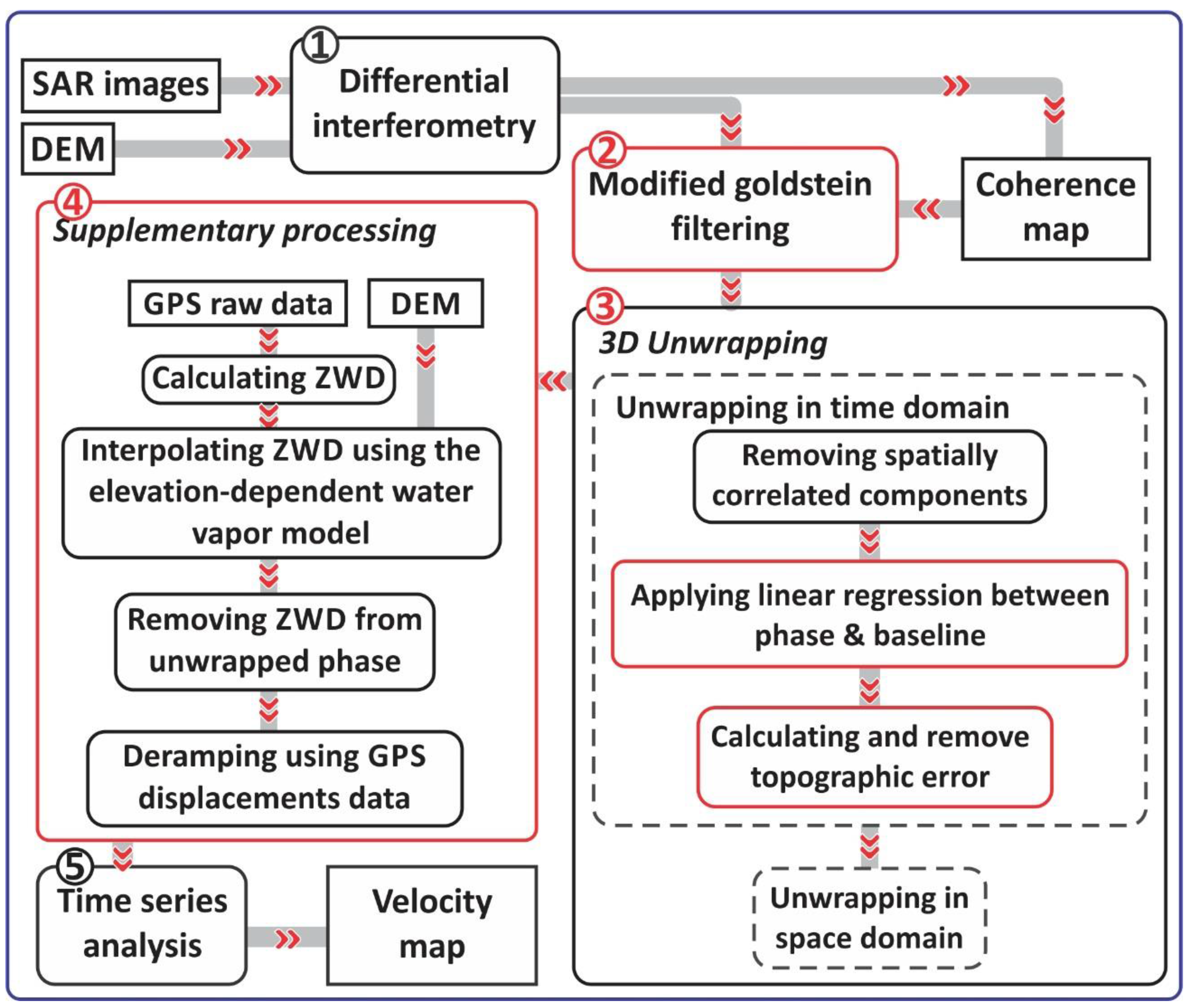
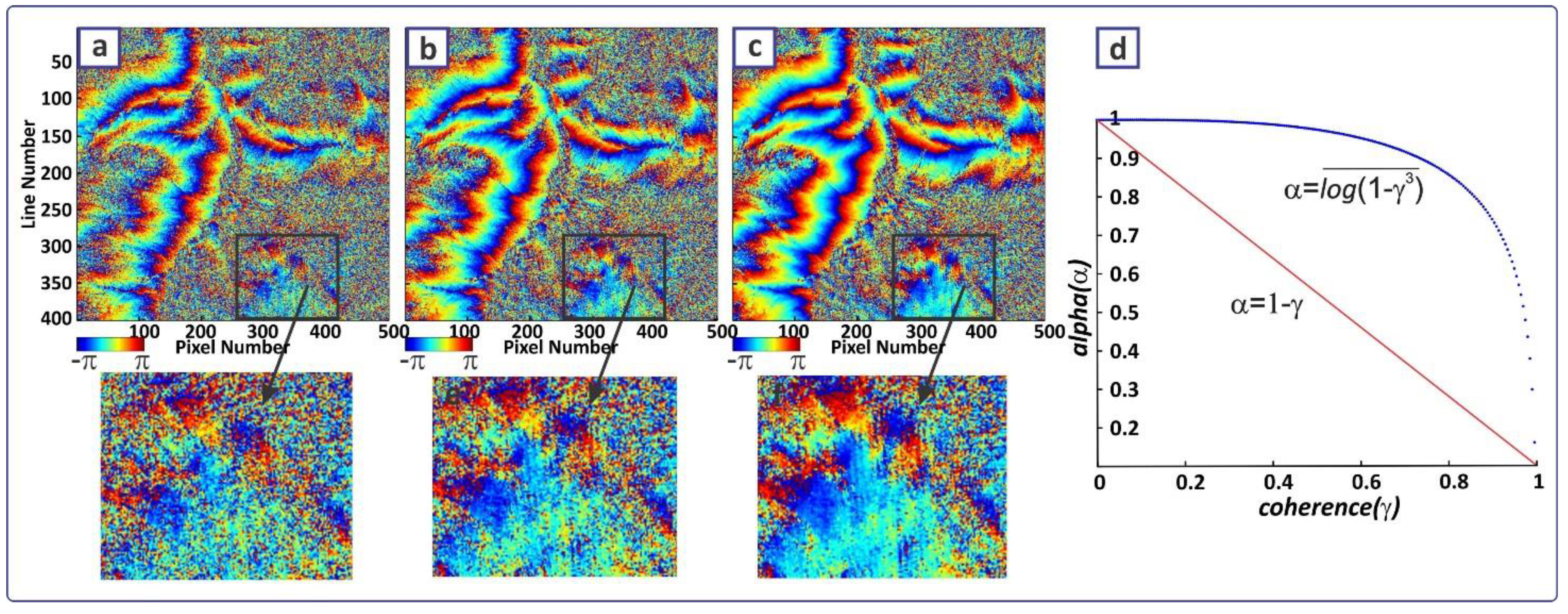
2.1. Modified Filtering
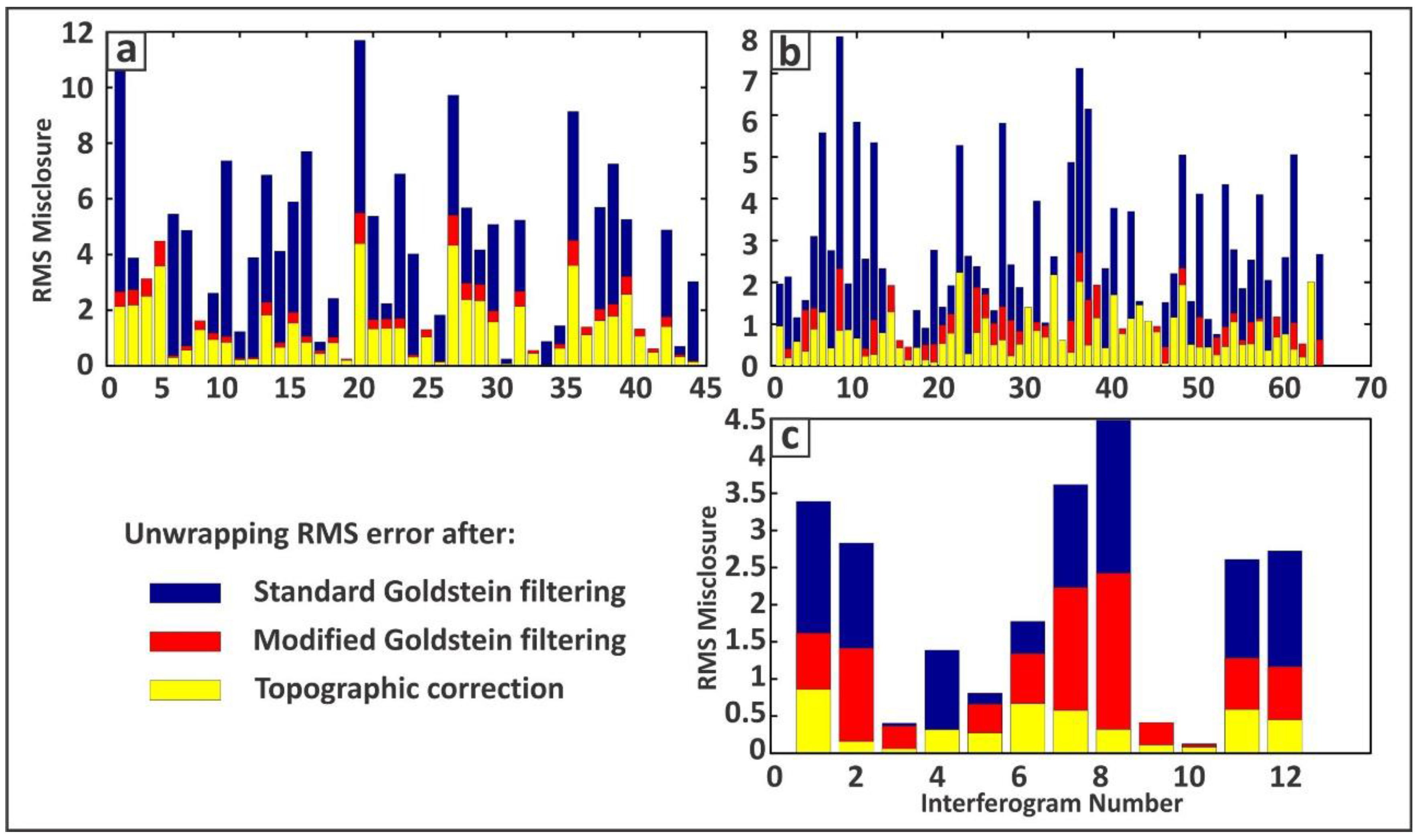
2.2. Improving the Interferometric Phase Unwrapping

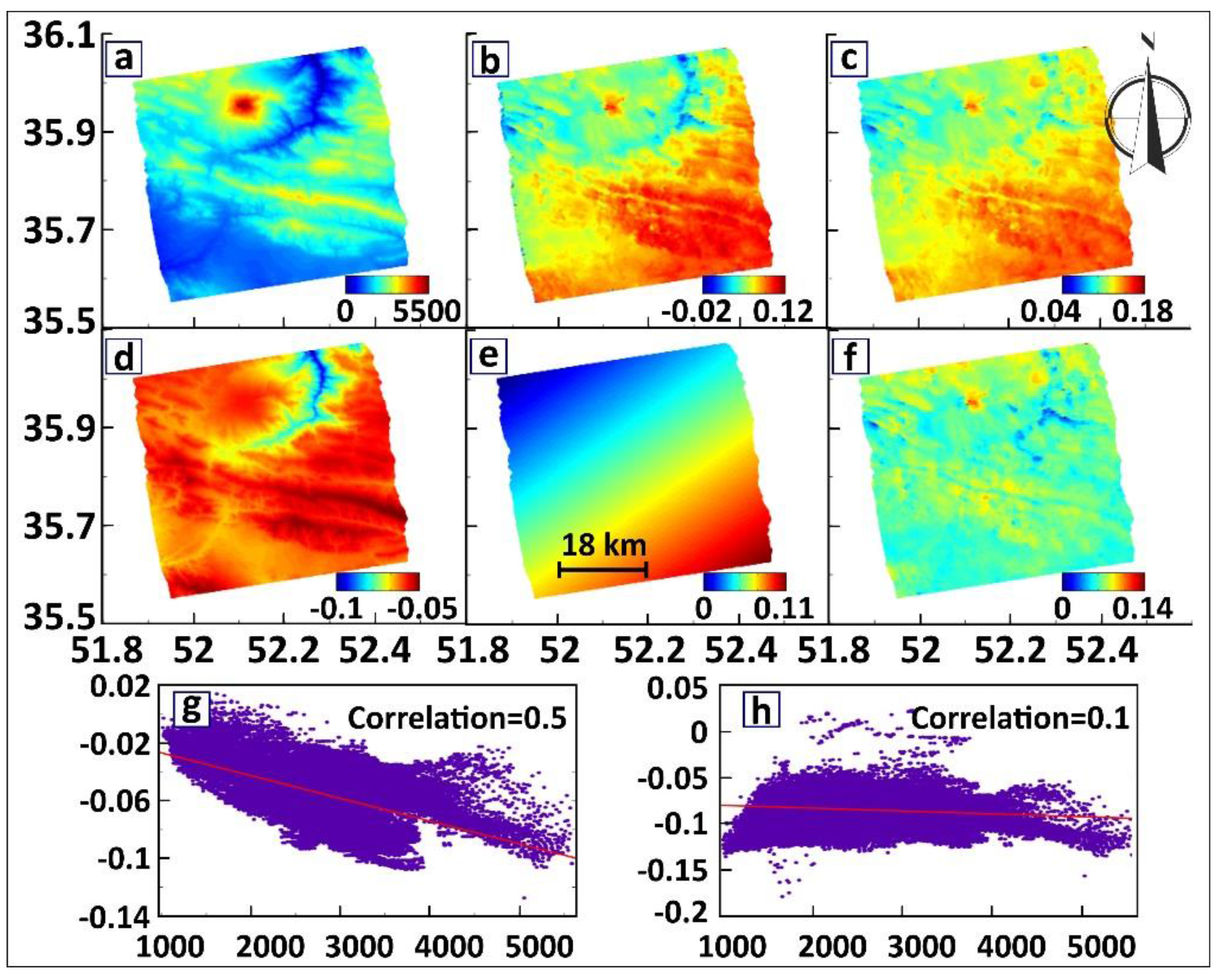
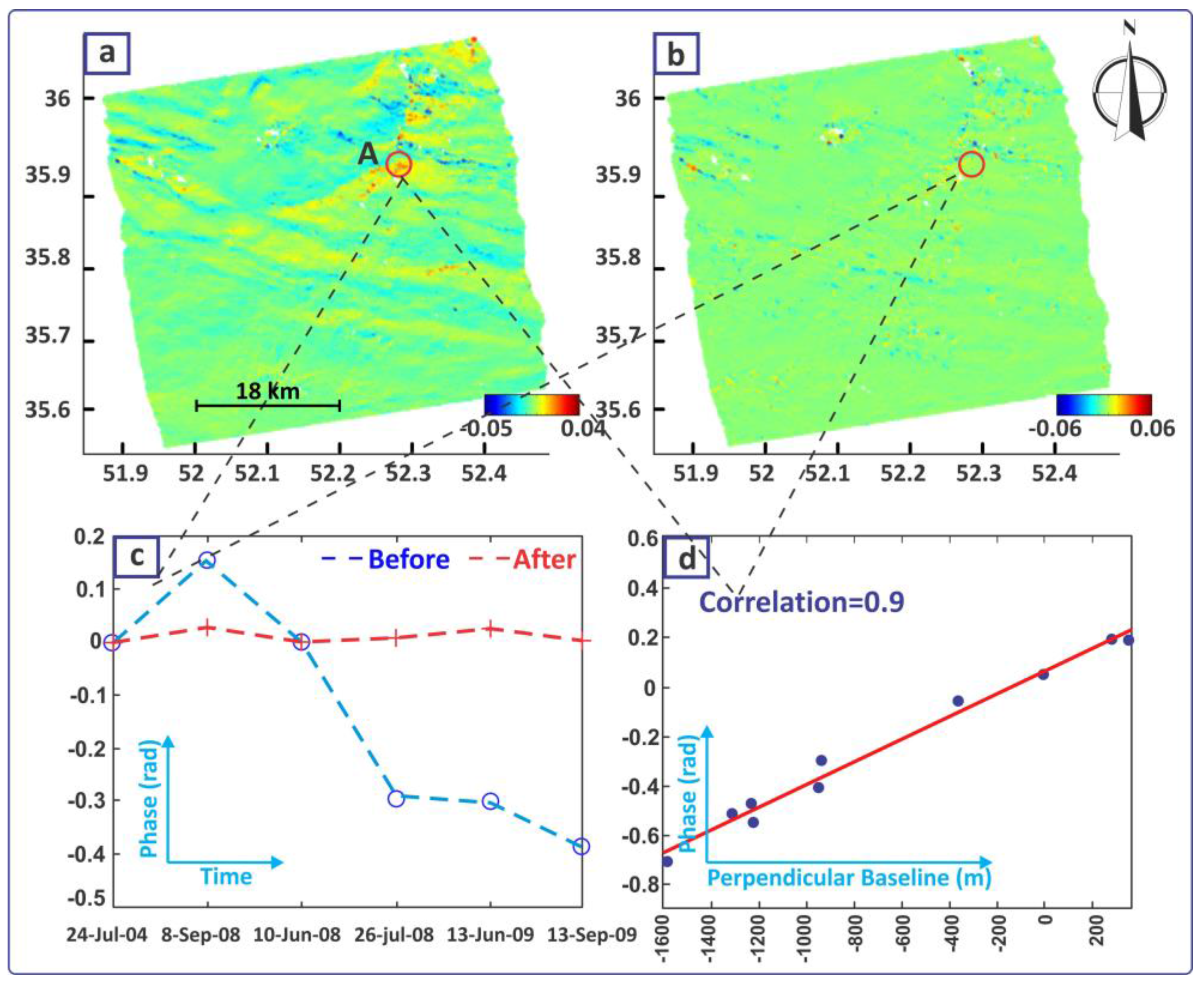
2.3. Supplementary Processing
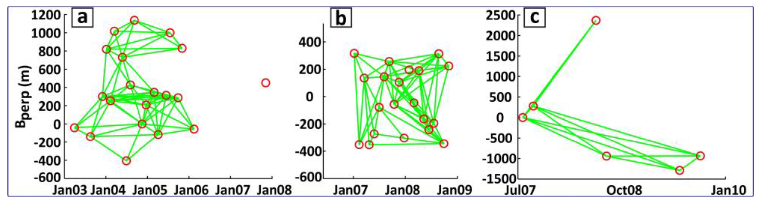
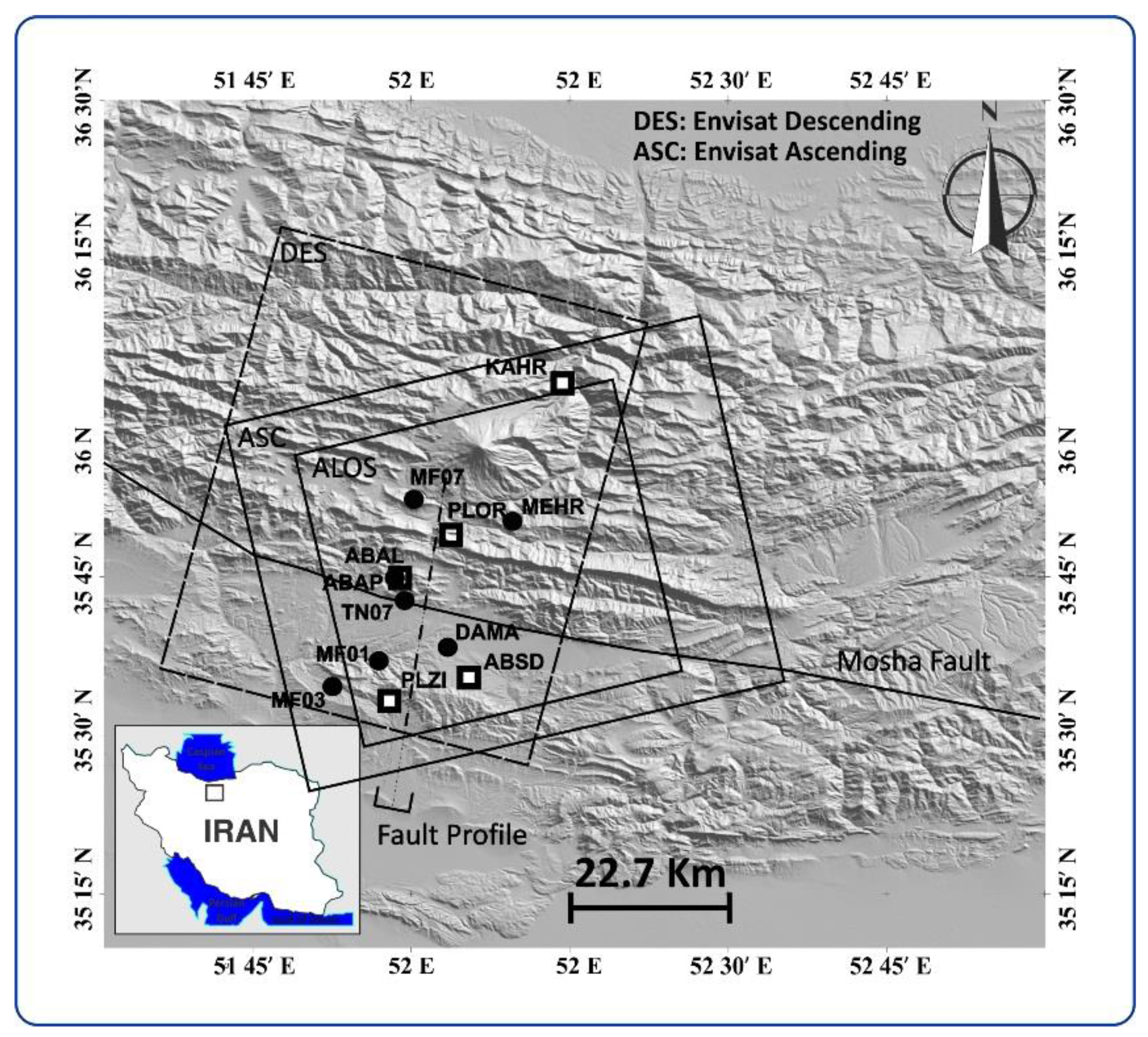
3. Experimental Study

StaMPS Processing vs. ISBAS Processing
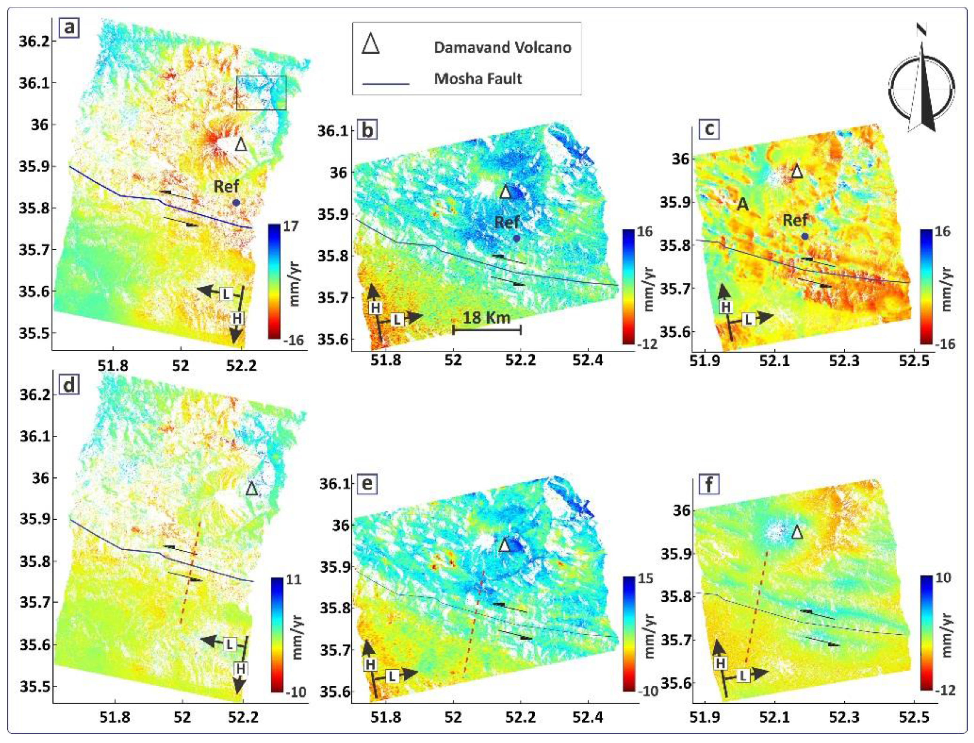
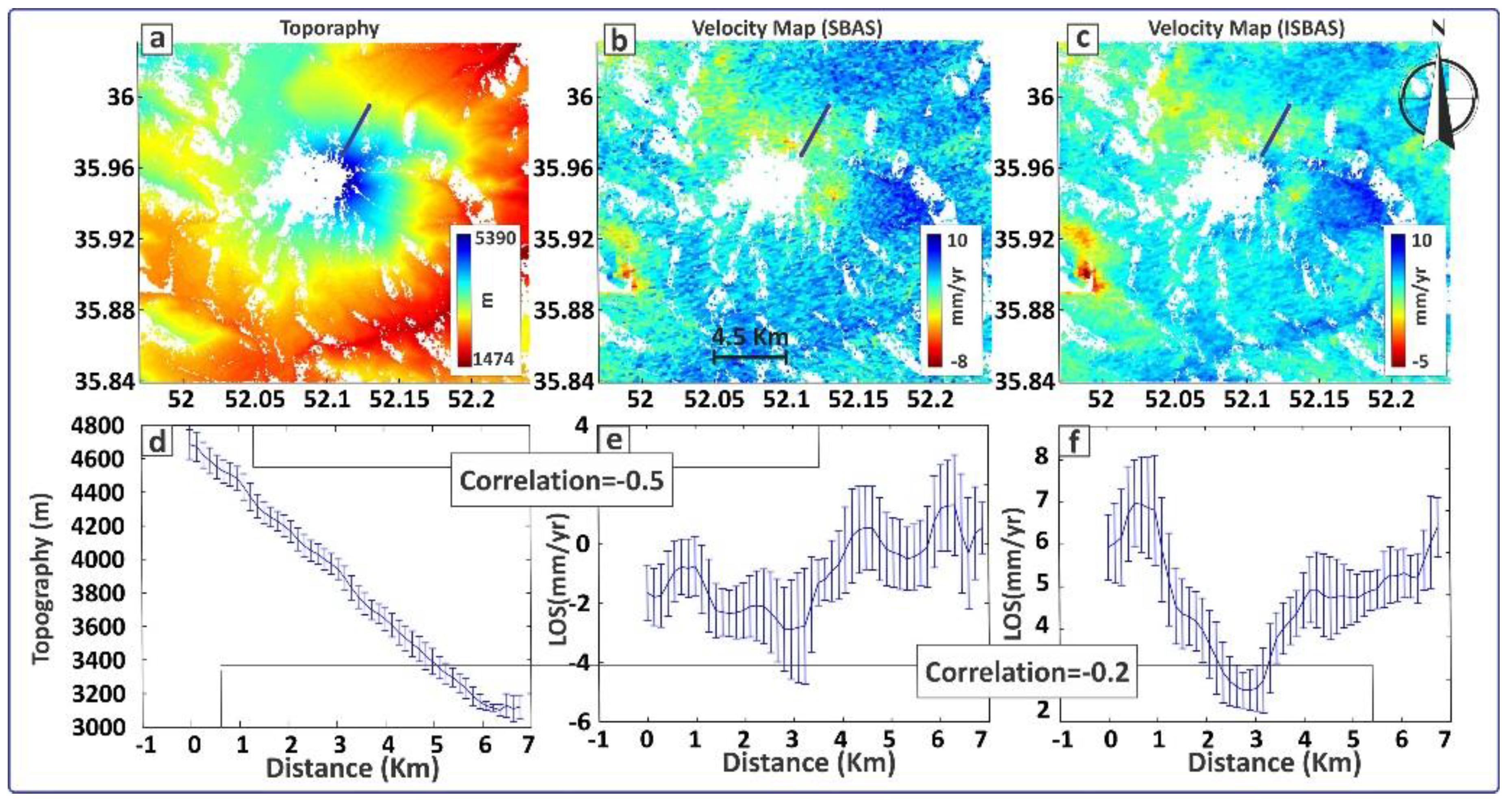
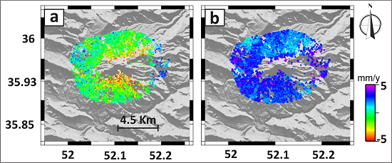
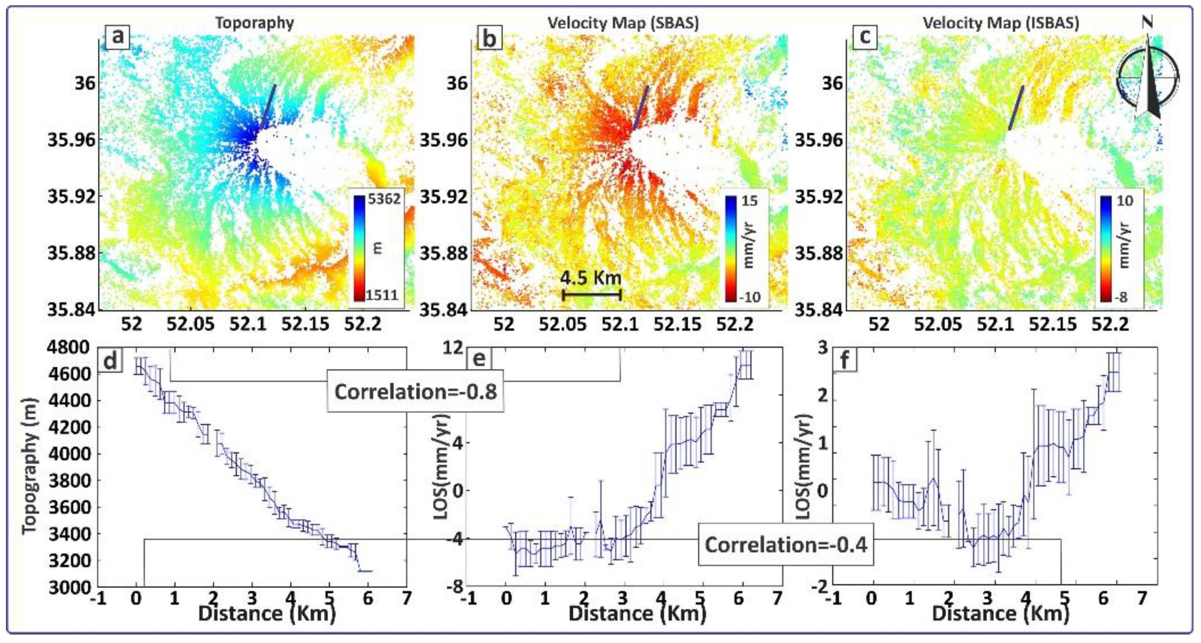
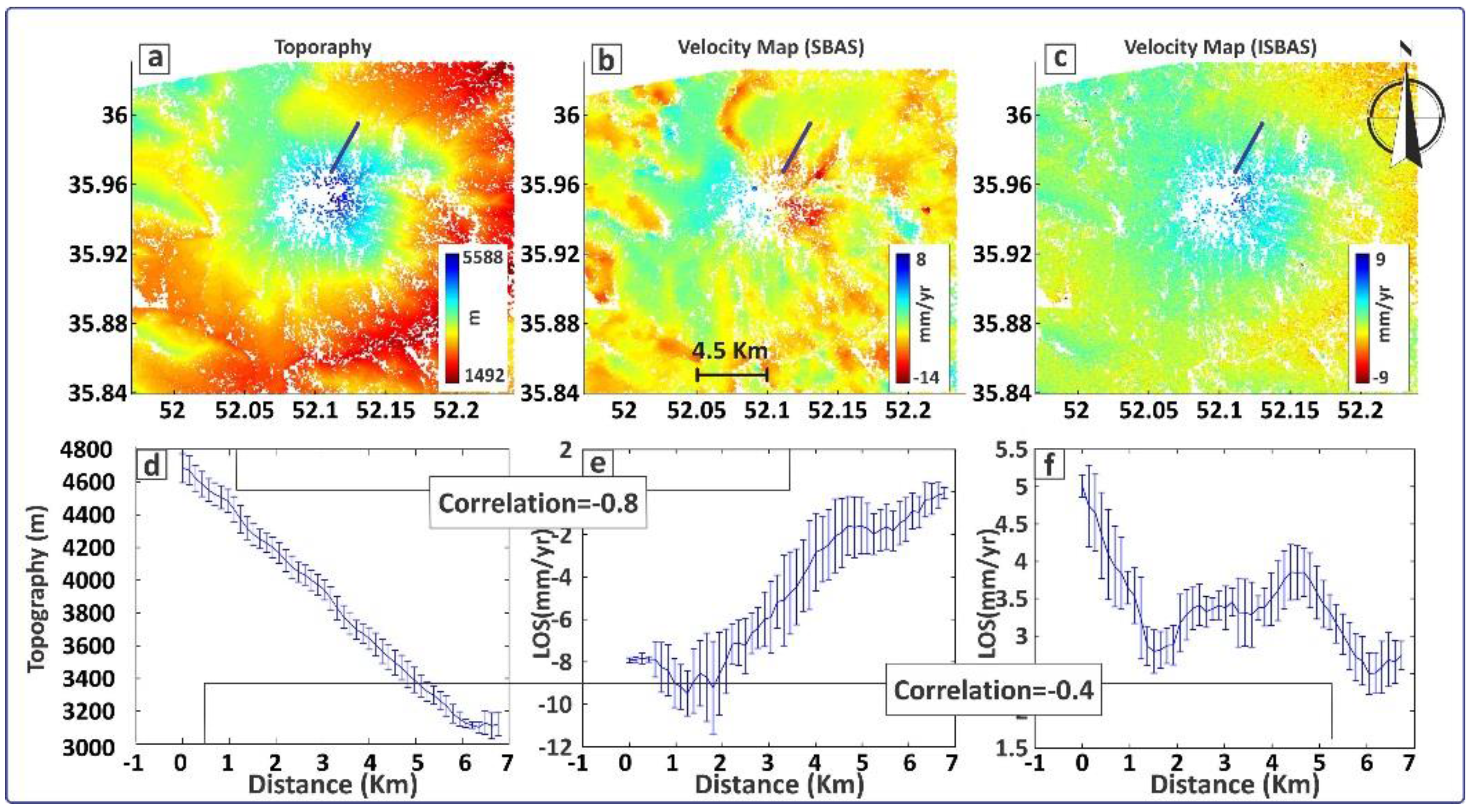
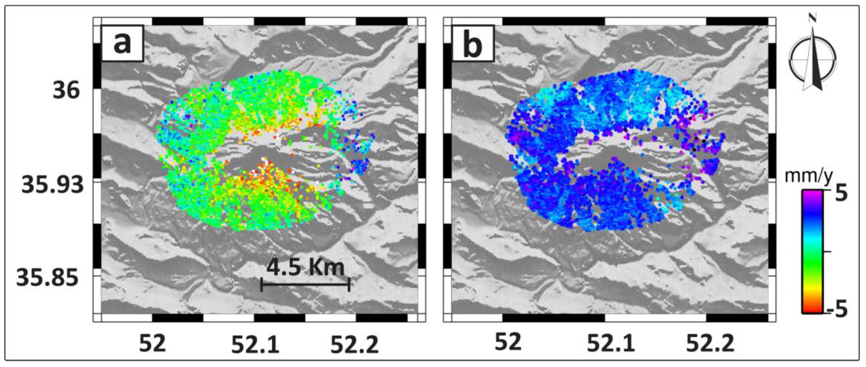
Damavand Volcano


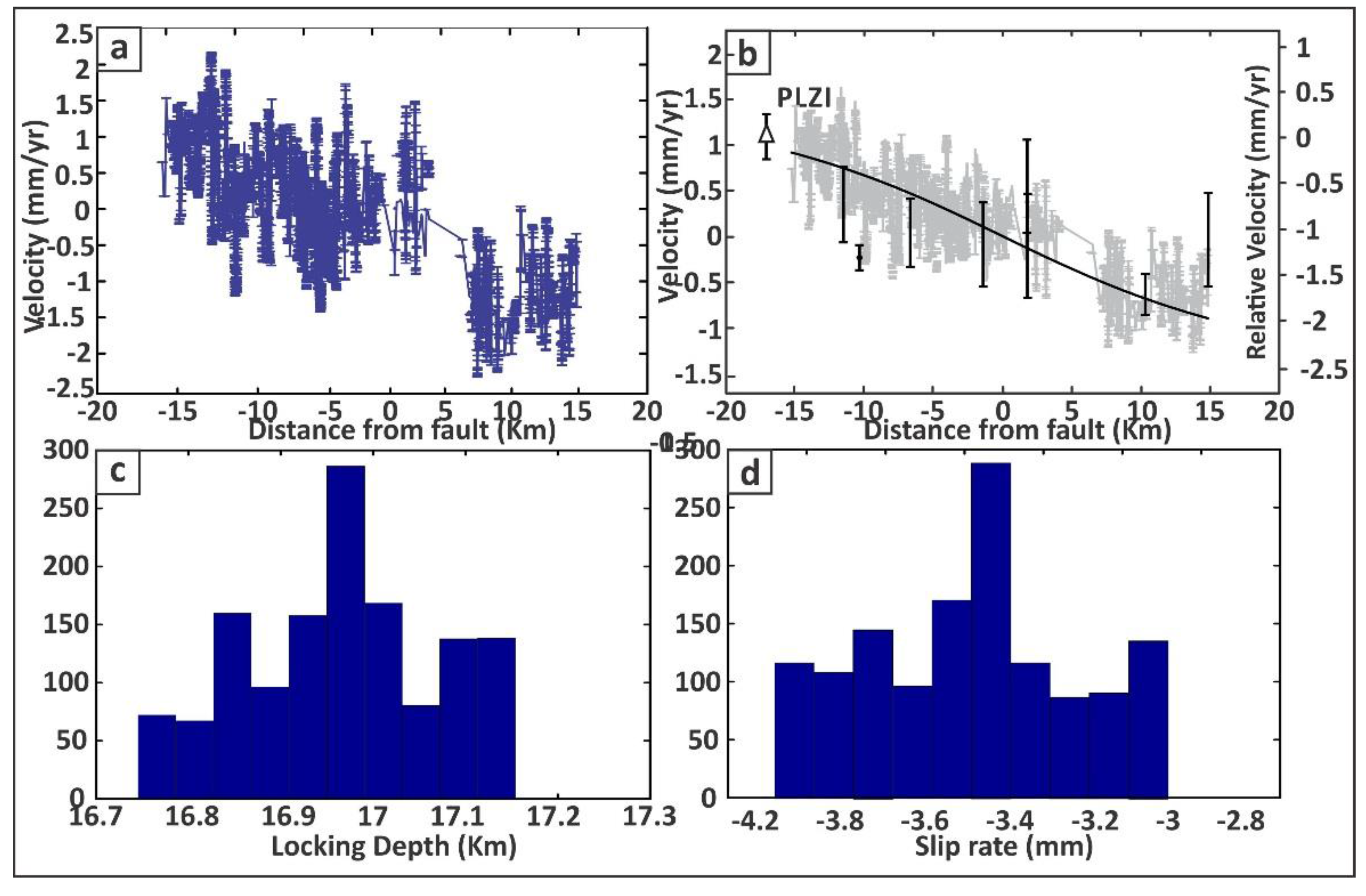
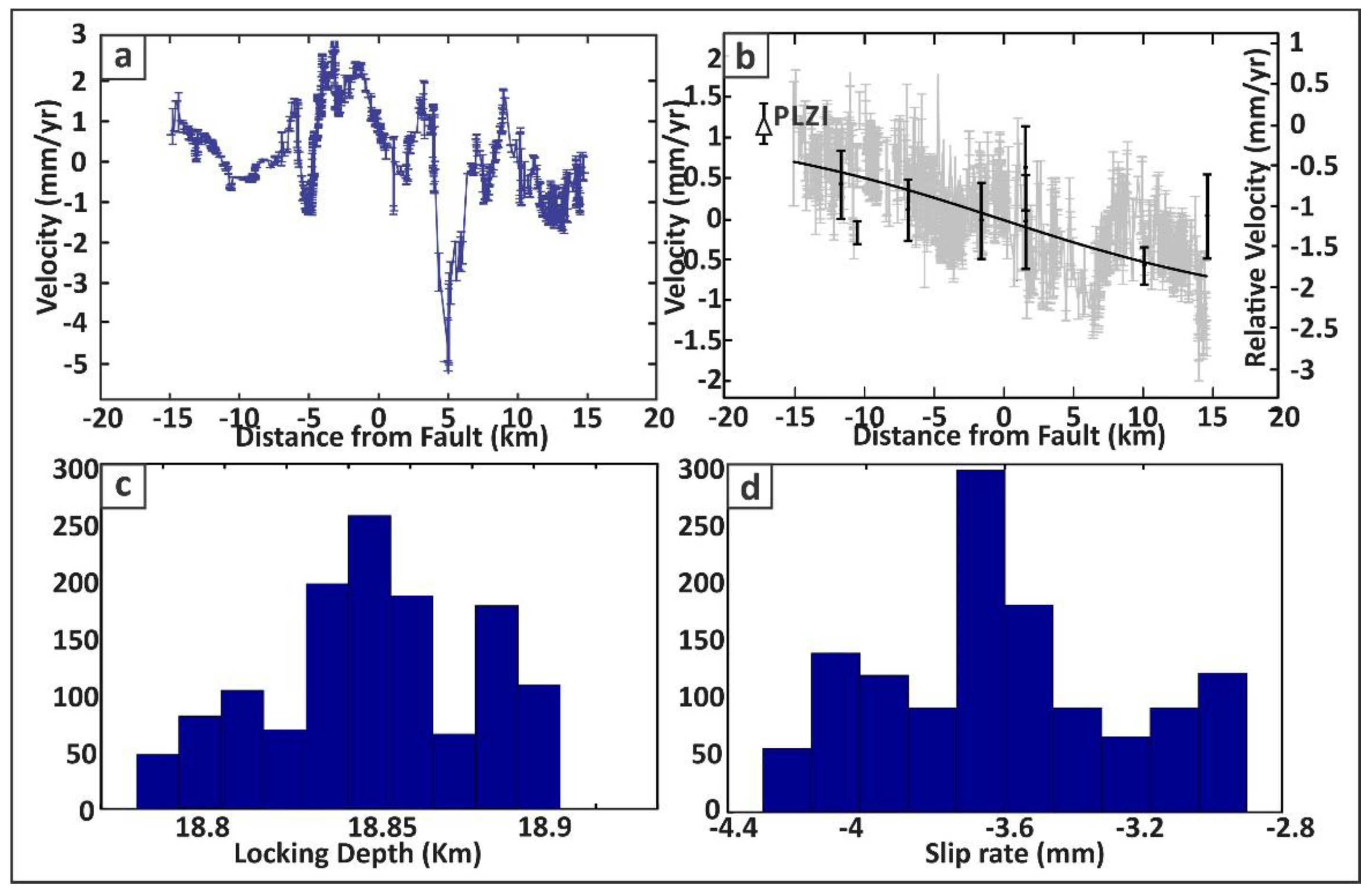
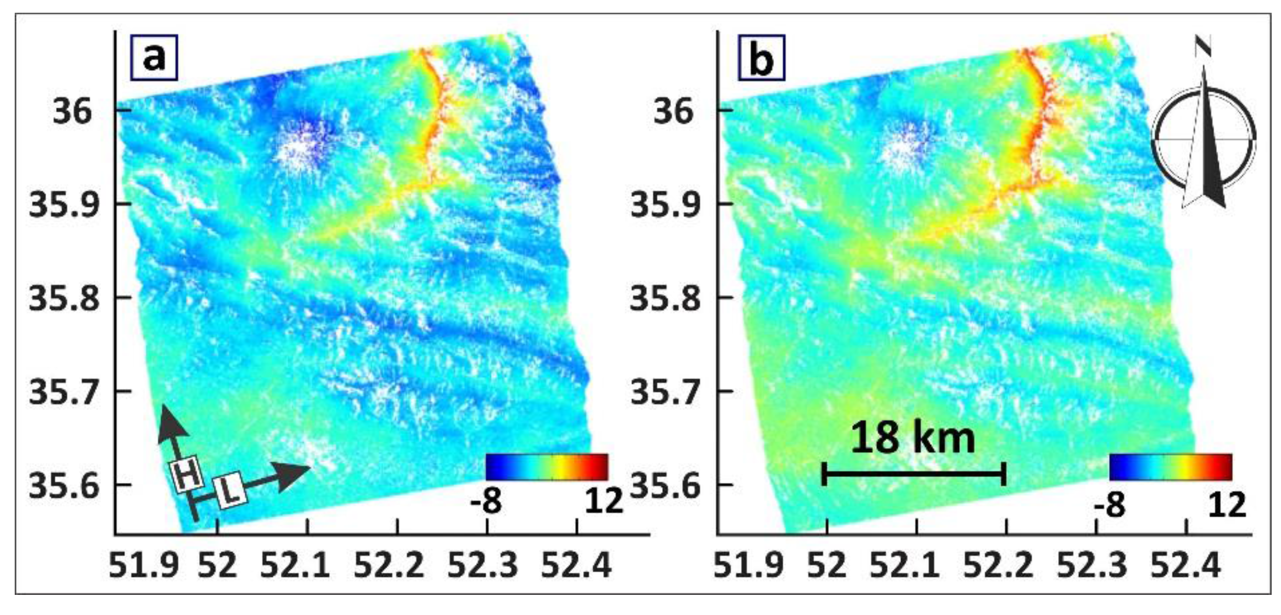
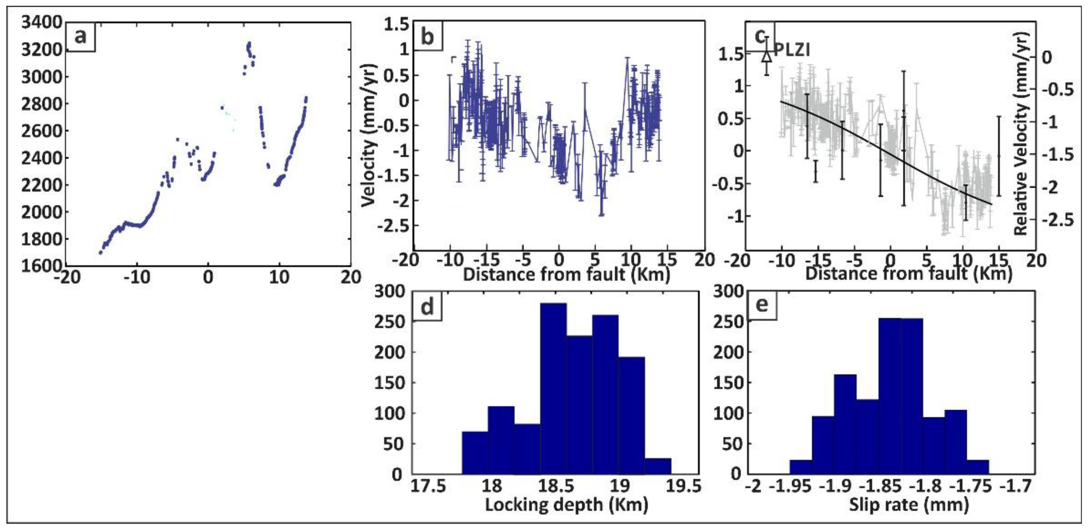
Mosha Fault

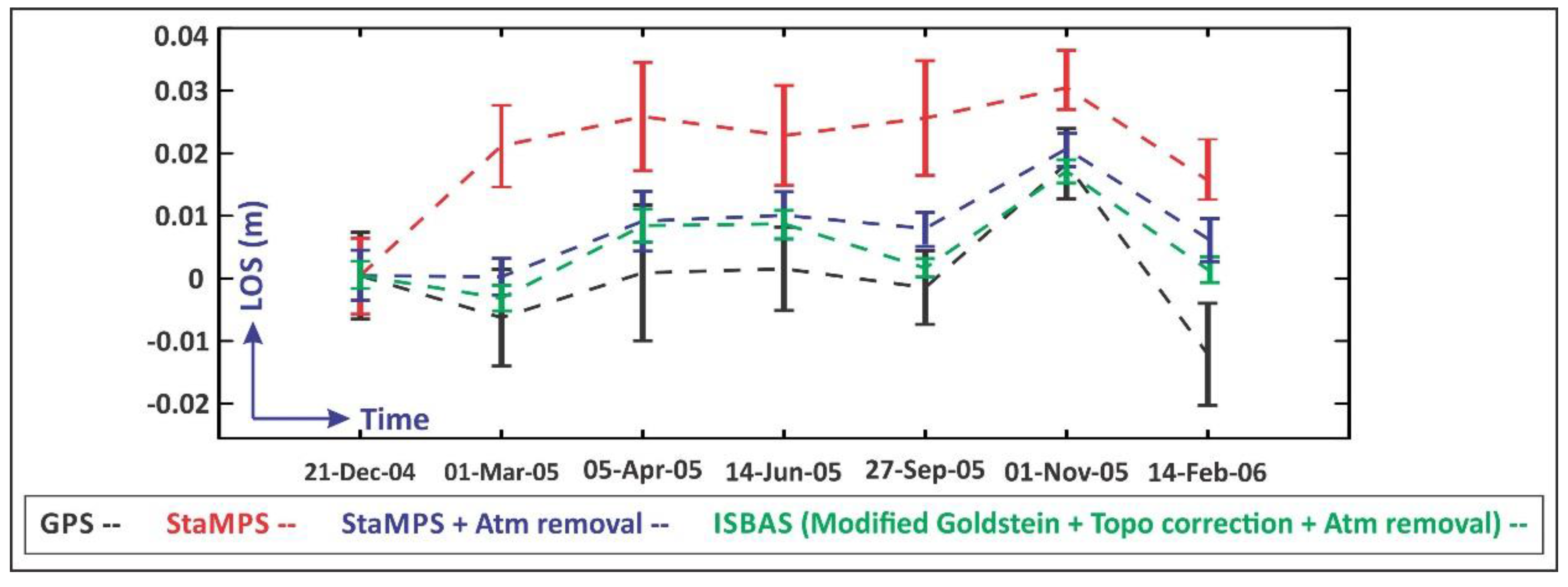
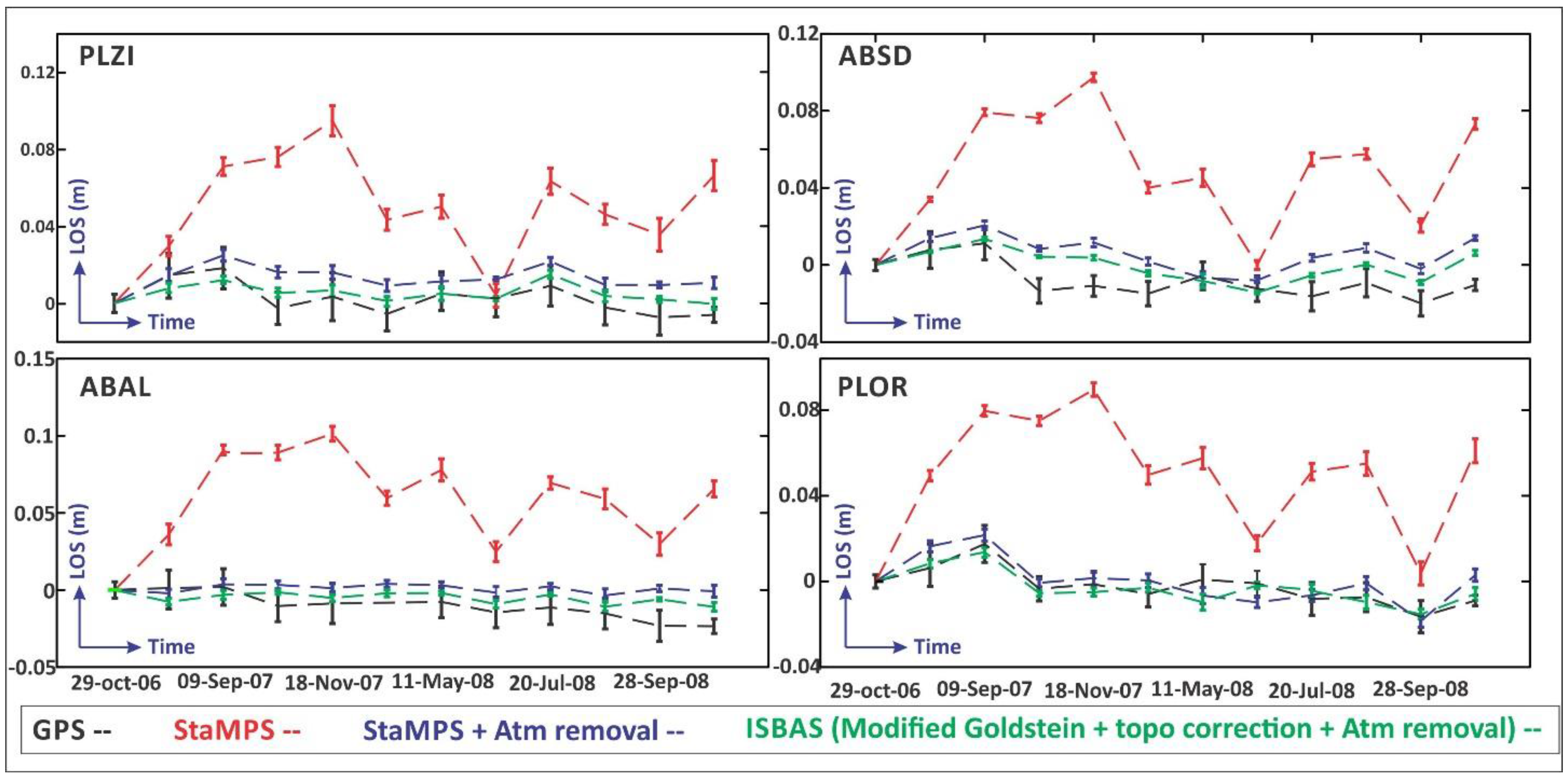
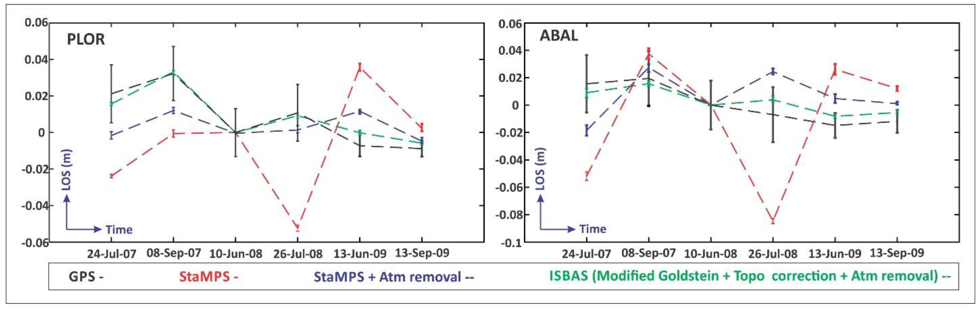
Comparison with GPS Observations
4. Discussion


| RMSE (cm) | |||||||
|---|---|---|---|---|---|---|---|
| Dataset → | Envisat descending | Envisat Ascending | ALOS | ||||
| Processing ↓ | PLOR | PLZI | ABSD | ABAL | PLOR | ABAL | PLOR |
| Stamps | 2.2 | 5.3 | 6.6 | 7.5 | 5.6 | 4.69 | 3.9 |
| Atm & Orb correction | 0.093 | 1.3 | 1.6 | 1.4 | 0.67 | 2.14 | 1.5 |
| ISBAS | 0.66 | 0.56 | 1.02 | 0.87 | 0.36 | 0.6 | 0.4 |
5. Conclusions
Acknowledgments
Author Contributions
Conflict of Interest
References
- Motagh, M.; Klotz, J.; Tavakoli, F.; Djamour, Y.; Arabi, S.; Wetzel, H.U.; Zschau, J. Combination of precise leveling and InSAR data to constrain source parameters of the mw = 6.5, 26 December 2003 Bam Earthquake. Pure Appl. Geophys. 2006, 163, 1–18. [Google Scholar] [CrossRef]
- Hooper, A.; Bekaert, D.; Spaans, K.; Arikan, M. Recent advances in SAR interferometry time series analysis for measuring crustal deformation. Tectonophysics 2012, 514–517, 1–13. [Google Scholar] [CrossRef]
- Caro Cuenca, M.; Hooper, A.J.; Hanssen, R.F. Surface deformation induced by water influx in the abandoned coal mines in Limburg, The Netherlands observed by satellite radar interferometry. J. Appl. Geophys. 2013, 88, 1–11. [Google Scholar] [CrossRef]
- Motagh, M.; Schurr, B.; Anderssohn, J.; Cailleau, B.; Walter, T.R.; Wang, R.; Villotte, J.P. Subduction earthquake deformation associated with 14 November 2007, mw 7.8 tocopilla earthquake in Chile: Results from InSAR and aftershocks. Tectonophysics 2010, 490, 60–68. [Google Scholar] [CrossRef]
- Motagh, M.; Beavan, J.; Fielding, E.J.; Haghshenas, M. Postseismic ground deformation following the september 2010 darfield, New Zealand, earthquake from TerraSAR-X, COSMO-SkyMed, and ALOS InSAR. IEEE Geosci. Remote Sens. Lett. 2014, 11, 186–190. [Google Scholar] [CrossRef]
- Hung, W.C.; Hwang, C.; Chen, Y.A.; Chang, C.P.; Yen, J.Y.; Hooper, A.; Yang, C.Y. Surface deformation from persistent scatterers SAR interferometry and fusion with leveling data: A case study over the Choushui River Alluvial Fan, Taiwan. Remote Sens. Environ. 2011, 115, 957–967. [Google Scholar] [CrossRef]
- Li, Z.W.; Xu, W.B.; Feng, G.C.; Hu, J.; Wang, C.C.; Ding, X.L.; Zhu, J.J. Correcting atmospheric effects on InSAR with MERIS water vapour data and elevation-dependent interpolation model. Geophys. J. Int. 2012, 189, 898–910. [Google Scholar] [CrossRef]
- Li, Z.; Fielding, E.J.; Cross, P. Integration of InSAR time-series analysis and water-vapor correction for mapping postseismic motion after the 2003 bam (Iran) earthquake. IEEE Trans. Geosci. Remote Sens. 2009, 47, 3220–3230. [Google Scholar]
- Li, Z.; Muller, J.P.; Cross, P.; Fielding, E.J. Interferometric synthetic aperture radar (InSAR) atmospheric correction: GPS, moderate resolution imaging spectroradiometer (MODIS), and InSAR integration. J. Geophys. Res.: Solid Earth 2005, 110. [Google Scholar] [CrossRef]
- Fornaro, G.; D’Agostino, N.; Giuliani, R.; Noviello, C.; Reale, D.; Verde, S. Assimilation of GPS-derived atmospheric propagation delay in DInSAR data processing. IEEE J. Sel. Top. Appl. Earth Obs. Remote Sens. 2014. [Google Scholar] [CrossRef]
- Zebker, H.A.; Villasenor, J. Decorrelation in interferometric radar echoes. IEEE Trans. Geosci. Remote Sens. 1992, 30, 950–959. [Google Scholar] [CrossRef]
- Hooper, A.; Segall, P.; Zebker, H. Persistent scatterer interferometric synthetic aperture radar for crustal deformation analysis, with application to Volcán Alcedo, Galápagos. J. Geophys. Res.: Solid Earth 2007, 112. [Google Scholar] [CrossRef]
- Hooper, A.J. A multi-temporal InSAR method incorporating both persistent scatterer and small baseline approaches. Geophys. Res. Lett. 2008, 35. [Google Scholar] [CrossRef]
- Motagh, M.; Wetzel, H.U.; Roessner, S.; Kaufmann, H. A TerraSAR-X InSAR study of landslides in southern Kyrgyzstan, central Asia. Remote Sens. Lett. 2013, 4, 657–666. [Google Scholar] [CrossRef]
- Ferretti, A.; Prati, C.; Rocca, F. Permanent scatterers in SAR interferometry. IEEE Trans. Geosci. Remote Sens. 2001, 39, 8–20. [Google Scholar] [CrossRef]
- Ferretti, A.; Savio, G.; Barzaghi, R.; Borghi, A.; Musazzi, S.; Novali, F.; Prati, C.; Rocca, F. Submillimeter accuracy of InSAR time series: Experimental validation. IEEE Trans. Geosci. Remote Sens. 2007, 45, 1142–1153. [Google Scholar] [CrossRef]
- Ferretti, A.; Prati, C.; Rocca, F. Nonlinear subsidence rate estimation using permanent scatterers in differential SAR interferometry. IEEE Trans. Geosci. Remote Sens. 2000, 38, 2202–2212. [Google Scholar] [CrossRef]
- Kampes, B.M. Displacement Parameter Estimation Using Permanent Scatterer Interferometry. Ph.D. Thesis, Delft University of Technology, Delft, The Netherlands, 2005. [Google Scholar]
- Hooper, A.; Zebker, H.; Segall, P.; Kampes, B. A new method for measuring deformation on volcanoes and other natural terrains using InSAR persistent scatterers. Geophys. Res. Lett. 2004, 31, 1–5. [Google Scholar] [CrossRef]
- Shanker, P.; Zebker, H. Persistent scatterer selection using maximum likelihood estimation. Geophys. Res. Lett. 2007, 34. [Google Scholar] [CrossRef]
- Ferretti, A.; Fumagalli, A.; Novali, F.; Prati, C.; Rocca, F.; Rucci, A. A new algorithm for processing interferometric data-stacks: Squeesar. IEEE Trans. Geosci. Remote Sens. 2011, 49, 3460–3470. [Google Scholar] [CrossRef]
- Motagh, M.; Hoffmann, J.; Kampes, B.; Baes, M.; Zschau, J. Strain accumulation across the gazikoy-saros segment of the north anatolian fault inferred from persistent scatterer interferometry and GPS measurements. Earth Planet. Sci. Lett. 2007, 255, 432–444. [Google Scholar] [CrossRef]
- Berardino, P.; Fornaro, G.; Lanari, R.; Sansosti, E. A new algorithm for surface deformation monitoring based on small baseline differential SAR interferograms. IEEE Trans. Geosci. Remote Sens. 2002, 40, 2375–2383. [Google Scholar] [CrossRef]
- Lanari, R.; Casu, F.; Manzo, M.; Zeni, G.; Berardino, P.; Manunta, M.; Pepe, A. An overview of the small baseline subset algorithm: A DInSAR technique for surface deformation analysis. Pure Appl. Geophys. 2007, 164, 637–661. [Google Scholar] [CrossRef]
- Lanari, R.; Mora, O.; Manunta, M.; Mallorquí, J.J.; Berardino, P.; Sansosti, E. A small-baseline approach for investigating deformations on full-resolution differential SAR interferograms. IEEE Trans. Geosci. Remote Sens. 2004, 42, 1377–1386. [Google Scholar] [CrossRef]
- Lauknes, T.R.; Zebker, H.A.; Larsen, Y. InSAR deformation time series using an-norm small-baseline approach. IEEE Trans. Geosci. Remote Sens. 2011, 49, 536–546. [Google Scholar] [CrossRef]
- Schmidt, D.A.; Bürgmann, R. Time-dependent land uplift and subsidence in the santa clara valley, California, from a large interferometric snthetic aperture radar data set. J. Geophys. Res.: Solid Earth 2003, 108. [Google Scholar] [CrossRef]
- Jolivet, R.; Grandin, R.; Lasserre, C.; Doin, M.P.; Peltzer, G. Systematic InSAR tropospheric phase delay corrections from global meteorological reanalysis data. Geophys. Res. Lett. 2011, 38. [Google Scholar] [CrossRef] [Green Version]
- Fornaro, G.; Reale, D.; Serafino, F. Four-dimensional SAR imaging for height estimation and monitoring of single and double scatterers. IEEE Trans. Geosci. Remote Sens. 2009, 47, 224–237. [Google Scholar] [CrossRef]
- Samsonov, S.; Tiampo, K. Time series analysis of subsidence at Tauhara and Ohaaki geothermal fields, New Zealand, observed by ALOS PALSAR interferometry during 2007–2009. Can. J. Remote Sens. 2010, 36, S327–S334. [Google Scholar] [CrossRef]
- Fattahi, H.; Amelung, F. Dem error correction in InSAR time series. IEEE Trans. Geosci. Remote Sens. 2013, 51, 4249–4259. [Google Scholar] [CrossRef]
- Samsonov, S. Topographic correction for ALOS PALSAR interferometry. IEEE Trans. Geosci. Remote Sens. 2010, 48, 3020–3027. [Google Scholar] [CrossRef]
- Pinel, V.; Hooper, A.; de la Cruz-Reyna, S.; Reyes-Davila, G.; Doin, M.P.; Bascou, P. The challenging retrieval of the displacement field from InSAR data for andesitic stratovolcanoes: Case study of Popocatepetl and Colima Volcano, Mexico. J. Volcanol. Geotherm. Res. 2011, 200, 49–61. [Google Scholar] [CrossRef]
- Hooper, A.J. Persistent Scatter Radar Interferometry for Crustal Deformation Studies and Modeling of Volcanic Deformation. Ph.D. Thesis, Stanford University, Stanford, CA, USA, 2006. [Google Scholar]
- Hooper, A.; Zebker, H.A. Phase unwrapping in three dimensions with application to InSAR time series. J. Opt. Soc. Am. A: Opt. Image Sci. Vis. 2007, 24, 2737–2747. [Google Scholar] [CrossRef]
- Hooper, A. Bayesian inversion of wrapped InSAR data for geophysical parameter estimation. In Proceedings of ESA Living Planet Symposium, Bergen, Norway, 28 June–2 July 2010.
- Goldstein, R.M.; Werner, C.L. Radar interferogram filtering for geophysical applications. Geophys. Res. Lett. 1998, 25, 4035–4038. [Google Scholar] [CrossRef]
- Baran, I.; Stewart, M.P.; Kampes, B.M.; Perski, Z.; Lilly, P. A modification to the goldstein radar interferogram filter. IEEE Trans. Geosci. Remote Sens. 2003, 41, 2114–2118. [Google Scholar] [CrossRef]
- Doin, M.P.; Lasserre, C.; Peltzer, G.; Cavalié, O.; Doubre, C. Corrections of stratified tropospheric delays in SAR interferometry: Validation with global atmospheric models. J. Appl. Geophys. 2009, 69, 35–50. [Google Scholar] [CrossRef]
- Pinel, V.; Hooper, A.; de la Cruz-Reyna, S.; Reyes-Davila, G.; Doin, M.P. Study of the Deformation Field of Two Active Mexican Stratovolcanoes (Popocatepetl and Colima Volcano) by Time Series of Insar Data; European Space Agency: Paris, France, 2008. [Google Scholar]
- Emardson, T.R.; Johansson, J.M. Spatial interpolation of the atmospheric water vapor content between sites in a ground-based GPS network. Geophys. Res. Lett. 1998, 25, 3347–3350. [Google Scholar] [CrossRef]
- Li, Z.; Fielding, E.J.; Cross, P.; Muller, J.P. Interferometric synthetic aperture radar atmospheric correction: GPS topography-dependent turbulence model. J. Geophys. Res.: Solid Earth 2006, 111. [Google Scholar] [CrossRef]
- Li, Z.; Ding, X.; Huang, C.; Wadge, G.; Zheng, D. Modeling of atmospheric effects on InSAR measurements by incorporating terrain elevation information. J. Atmos. Sol. Terr. Phys. 2006, 68, 1189–1194. [Google Scholar] [CrossRef]
- Xu, W.; Li, Z.; Ding, X.; Zhu, J. Interpolating atmospheric water vapor delay by incorporating terrain elevation information. J. Geod. 2011, 85, 555–564. [Google Scholar] [CrossRef]
- Onn, F.; Zebker, H. Correction for interferometric synthetic aperture radar atmospheric phase artifacts using time series of zenith wet delay observations from a GPS network. J. Geophys. Res. Solid Earth 2006, 111. [Google Scholar] [CrossRef]
- Zumberge, J.; Heflin, M.; Jefferson, D.; Watkins, M.; Webb, F.H. Precise point positioning for the efficient and robust analysis of GPS data from large networks. J. Geophys. Res.: Solid Earth 1997, 102, 5005–5017. [Google Scholar] [CrossRef]
- Sharifi, M.; Souri, A. A hybrid LS-HE and LS-SVM model to predict time series of precipitable water vapor derived from GPS measurements. Arabian J. Geosci. 2014. [Google Scholar] [CrossRef]
- Agram, P.S. Persistent Scatterer Interferometry in Natural Terrain. Ph.D. Thesis, Stanford University, Stanford, CA, USA, 2010. [Google Scholar]
- Samieie-Esfahany, S.; Hanssen, R.; van Thienen-Visser, K.; Muntendam-Bos, A. On the effect of horizontal deformation on InSAR subsidence estimates. In Proceedings of the Fringe 2009 Workshop, Frascati, Italy, 30 November–4 December 2009.
- Djamour, Y.; Vernant, P.; Bayer, R.; Nankali, H.R.; Ritz, J.; Hinderer, J.; Hatam, Y.; Luck, B.; Le Moigne, N.; Sedighi, M.; et al. GPS and gravity constraints on continental deformation in the Alborz Mountain Range, Iran. Geophys. J. Int. 2010, 183, 1287–1301. [Google Scholar] [CrossRef]
- Savage, J.; Burford, R. Accumulation of tectonic strain in California. Bull. Seismol. Soc. Am. 1970, 60, 1877–1896. [Google Scholar]
- Haupt, R.L.; Haupt, S.E. Practical Genetic Algorithms; John Wiley & Sons: Hoboken, NJ, USA, 2004. [Google Scholar]
- Cressie, N. Statistics for Spatial Data: Wiley Series in Probability and Statistics; Wiley-Interscience: Hoboken, NJ, USA, 1993. [Google Scholar]
- Mora, O.; Mallorqui, J.J.; Broquetas, A. Linear and nonlinear terrain deformation maps from a reduced set of interferometric SAR images. IEEE Trans. Geosci. Remote Sens. 2003, 41, 2243–2253. [Google Scholar] [CrossRef]
- Biescas, E.; Crosetto, M.; Agudo, M.; Monserrat, O.; Crippa, B. Two radar interferometric approaches to monitor slow and fast land deformation. J. Surv. Eng. 2007, 133, 66–71. [Google Scholar] [CrossRef]
- Yazdanparast, M.; Vosooghi, B. A research on damavand magma source model using GPS data. Geomat. Nat. Hazards Risk 2014, 5, 26–40. [Google Scholar] [CrossRef]
- Nilforoushan, F.; Masson, F.; Vernant, P.; Vigny, C.; Martinod, J.; Abbassi, M.; Nankali, H.; Hatzfeld, D.; Bayer, R.; Tavakoli, F.; et al. GPS network monitors the Arabia-Eurasia collision deformation in Iran. J. Geod. 2003, 77, 411–422. [Google Scholar] [CrossRef]
- Vernant, P.; Nilforoushan, F.; Chéry, J.; Bayer, R.; Djamour, Y.; Masson, F.; Nankali, H.; Ritz, J.F.; Sedighi, M.; Tavakoli, F. Deciphering oblique shortening of central Alborz in Iran using geodetic data. Earth Planet. Sci. Lett. 2004, 223, 177–185. [Google Scholar] [CrossRef]
- Ritz, J.; Balescu, S.; Soleymani, S.; Abbassi, M.; Nazari, H.; Feghhi, K.; Shabanian, E.; Tabassi, H.; Farbod, Y.; Lamothe, M. Determining the long-term slip rate along the Mosha Fault, Central Alborz, Iran. Implications in terms of seismic activity. In Proceeding of the 4th International Conference on Seismology and Earthquake Engeneering, Tehran, Iran, 12–14 May 2003.
- Peyret, M.; Djamour, Y.; Rizza, M.; Ritz, J.F.; Hurtrez, J.E.; Goudarzi, M.A.; Nankali, H.; Chéry, J.; le Dortz, K.; Uri, F. Monitoring of the large slow kahrod landslide in Alborz Mountain Range (Iran) by GPS and SAR interferometry. Eng. Geol. 2008, 100, 131–141. [Google Scholar] [CrossRef]
- Allen, M.B.; Ghassemi, M.R.; Shahrabi, M.; Qorashi, M. Accommodation of late cenozoic oblique shortening in the Alborz Range, northern Iran. J. Struct. Geol. 2003, 25, 659–672. [Google Scholar] [CrossRef]
- Zanchi, A.; Berra, F.; Mattei, M.; Ghassemi, M.R.; Sabouri, J. Inversion tectonics in central Alborz, Iran. J. Struct. Geol. 2006, 28, 2023–2037. [Google Scholar] [CrossRef]
- Yassaghi, A.; Madanipour, S. Influence of a transverse basement fault on along-strike variations in the geometry of an inverted normal fault: Case study of the mosha fault, central Alborz Range, Iran. J. Struct. Geol. 2008, 30, 1507–1519. [Google Scholar] [CrossRef]
- Ashtari, M.; Hatzfeld, D.; Kamalian, N. Microseismicity in the region of tehran. Tectonophysics 2005, 395, 193–208. [Google Scholar] [CrossRef]
© 2015 by the authors; licensee MDPI, Basel, Switzerland. This article is an open access article distributed under the terms and conditions of the Creative Commons Attribution license (http://creativecommons.org/licenses/by/4.0/).
Share and Cite
Vajedian, S.; Motagh, M.; Nilfouroushan, F. StaMPS Improvement for Deformation Analysis in Mountainous Regions: Implications for the Damavand Volcano and Mosha Fault in Alborz. Remote Sens. 2015, 7, 8323-8347. https://doi.org/10.3390/rs70708323
Vajedian S, Motagh M, Nilfouroushan F. StaMPS Improvement for Deformation Analysis in Mountainous Regions: Implications for the Damavand Volcano and Mosha Fault in Alborz. Remote Sensing. 2015; 7(7):8323-8347. https://doi.org/10.3390/rs70708323
Chicago/Turabian StyleVajedian, Sanaz, Mahdi Motagh, and Faramarz Nilfouroushan. 2015. "StaMPS Improvement for Deformation Analysis in Mountainous Regions: Implications for the Damavand Volcano and Mosha Fault in Alborz" Remote Sensing 7, no. 7: 8323-8347. https://doi.org/10.3390/rs70708323
APA StyleVajedian, S., Motagh, M., & Nilfouroushan, F. (2015). StaMPS Improvement for Deformation Analysis in Mountainous Regions: Implications for the Damavand Volcano and Mosha Fault in Alborz. Remote Sensing, 7(7), 8323-8347. https://doi.org/10.3390/rs70708323