
Mapping Secondary Forest Succession on Abandoned Agricultural Land with LiDAR Point Clouds and Terrestrial Photography

Abstract
:
1. Introduction
2. Materials and Methods
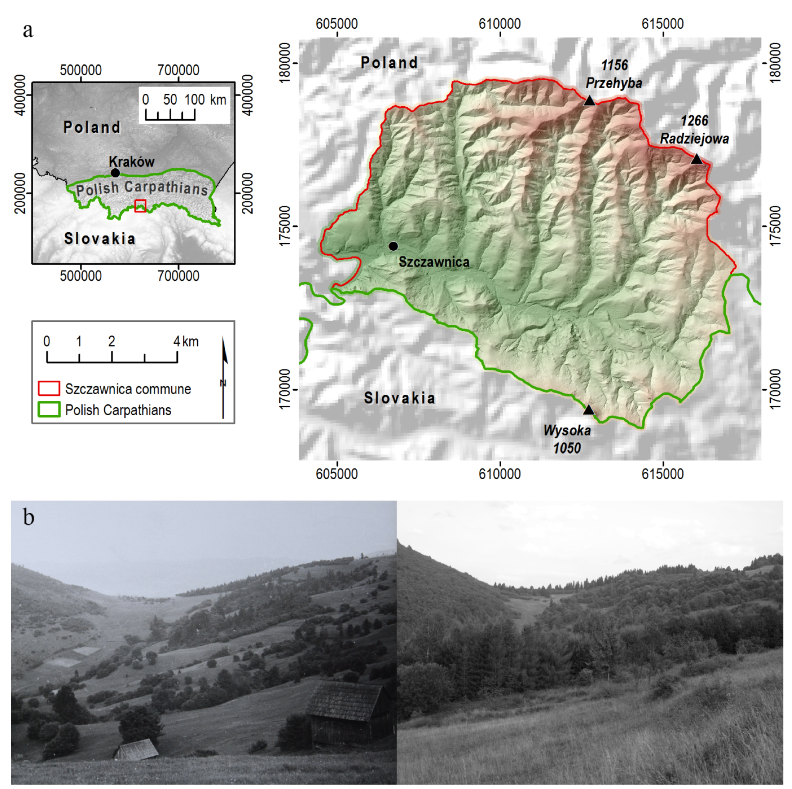
2.1. Study Area
2.2. Data

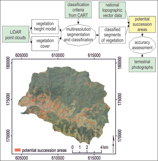
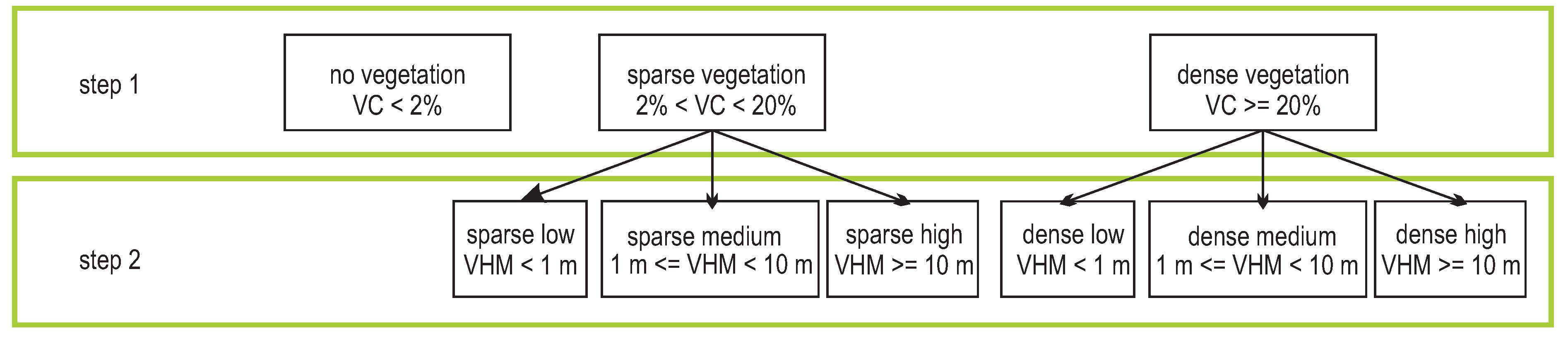
2.3. ALS Processing

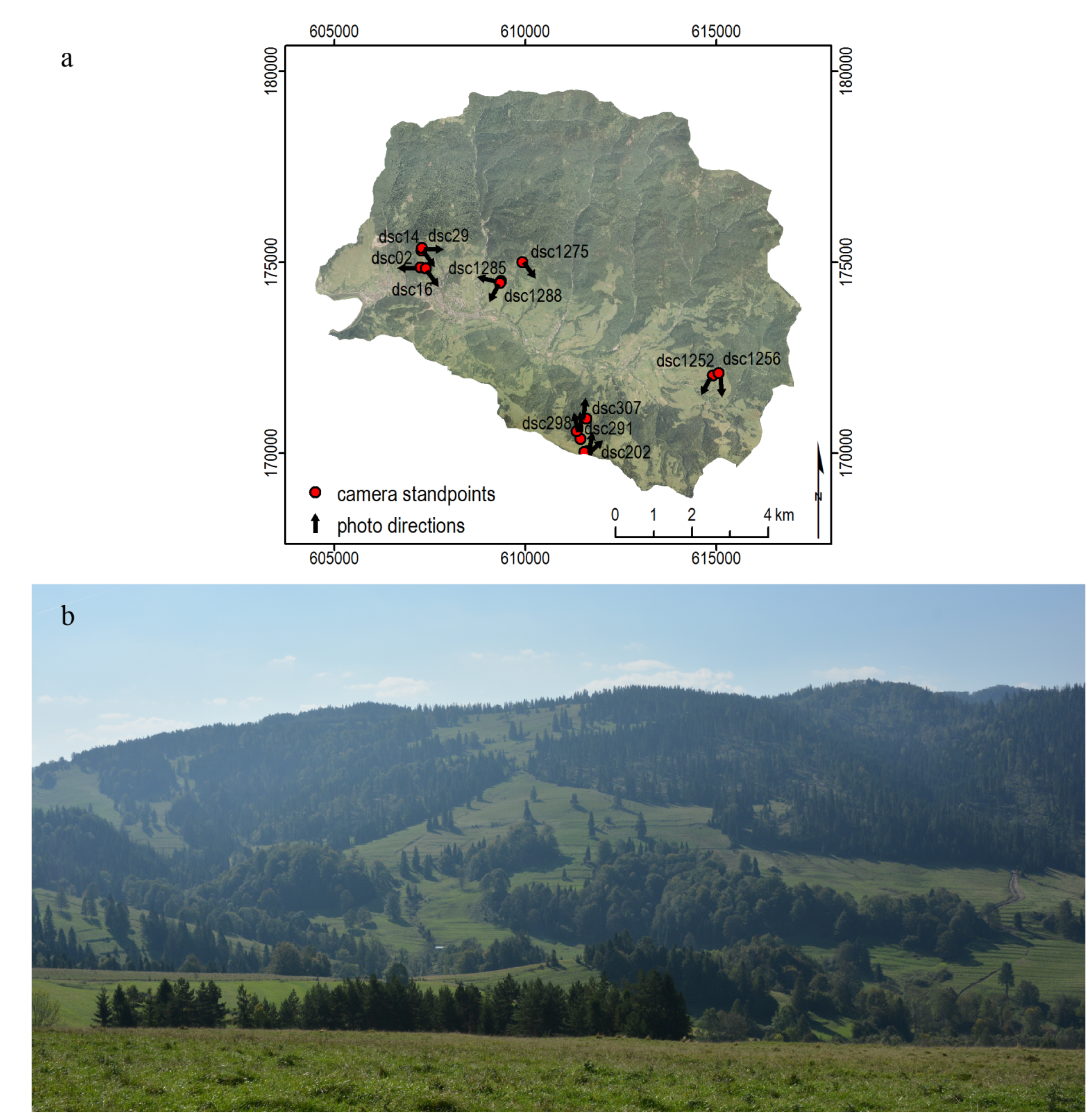
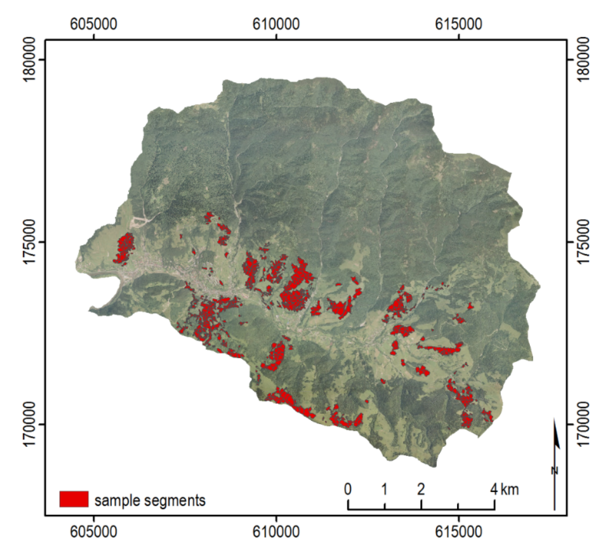
2.4. Accuracy Assessment

3. Results
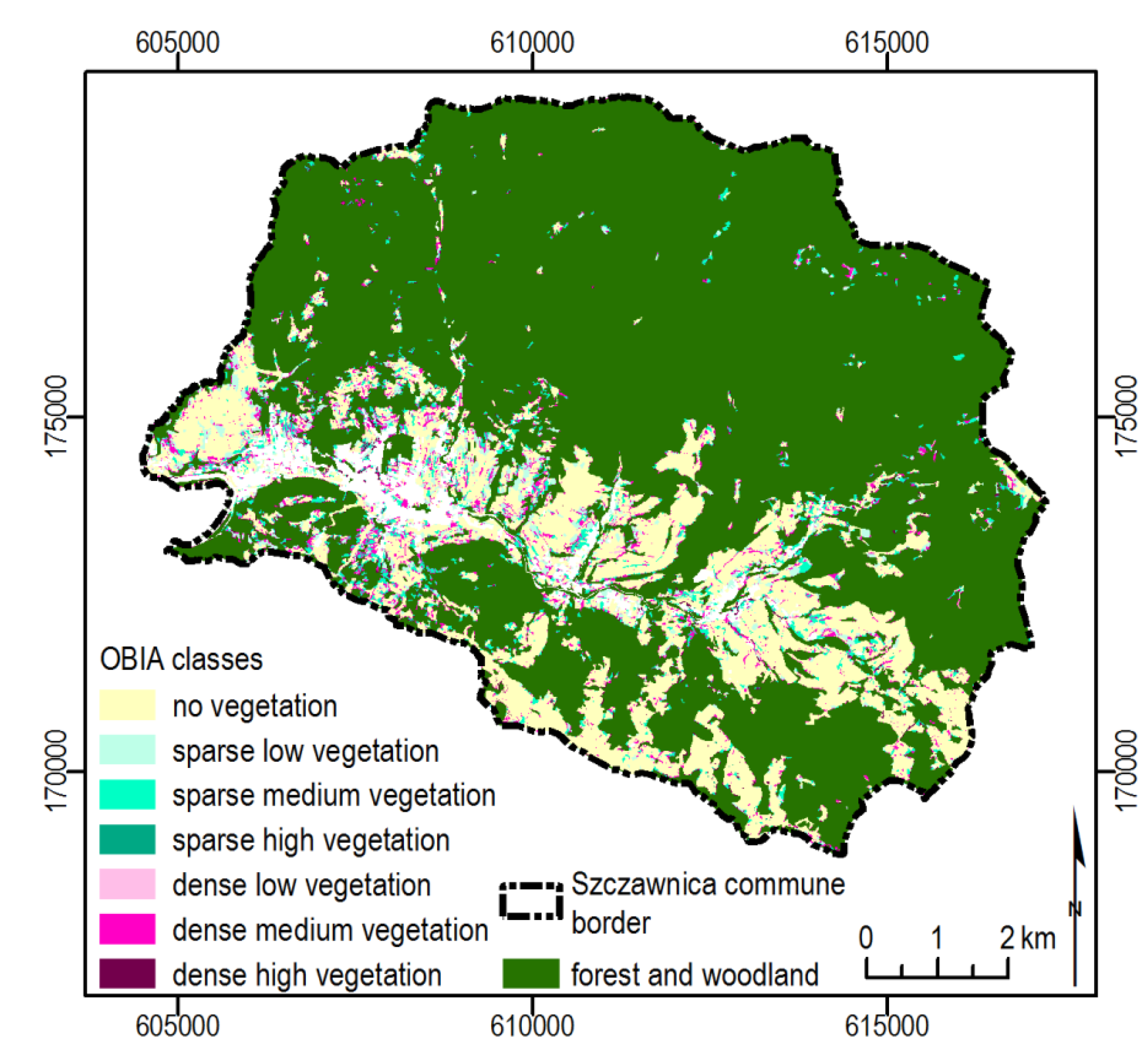
3.1. Object-Based Classification of LiDAR Data

| OBIA Class | Number of Classified Objects | Mean Area of Classified Objects [m2] | % of Analyzed Area | Number of Classified Objects in Sample Used for the Accuracy Assessment |
|---|---|---|---|---|
| no veg. | 2936 | 5254 | 18.21 | 529 |
| sparse low veg. | 917 | 2465 | 2.67 | 141 |
| sparse medium veg. | 4821 | 1510 | 8.59 | 172 |
| sparse high veg. | 1137 | 999 | 1.34 | 0 |
| dense low veg. | 30 | 957 | 0.03 | 0 |
| dense medium veg. | 8823 | 1625 | 16.92 | 135 |
| dense high veg. | 18270 | 2423 | 52.24 | 12 |
| Total | 36934 | 100 | 989 |
3.2. Relationships between the BDOT10k and LiDAR-Based Classification

| BDOT10k Class OBIA Class | Arable Land | Grassland | Forest, Woodland and Grove | Shrubland | Total | ||||
|---|---|---|---|---|---|---|---|---|---|
| % of SA | % of BDOT10k | % of SA | % of BDOT10k | % of SA | % of BDOT10k | % of SA | % of BDOT10k | % of SA | |
| no vegetation | 8.9 | 81.3 | 8.4 | 59.6 | 0.9 | 1.2 | 0.0 | 5.7 | 18.2 |
| sparse low veg | 0.8 | 6.7 | 1.4 | 10.0 | 0.5 | 0.7 | 0.0 | 10.4 | 2.7 |
| sparse medium veg | 0.5 | 4.9 | 2.0 | 14.2 | 6.0 | 8.0 | 0.0 | 25.7 | 8.5 |
| sparse high veg | 0.0 | 0.0 | 0.0 | 0.1 | 1.3 | 1.8 | 0.0 | 0.0 | 1.3 |
| dense low veg | 0.0 | 0.1 | 0.0 | 0.1 | 0.0 | 0.0 | 0.0 | 0.0 | 0.0 |
| dense medium veg | 0.6 | 5.6 | 1.7 | 12.1 | 14.5 | 19.4 | 0.1 | 57.2 | 16.9 |
| dense high veg | 0.2 | 1.4 | 0.6 | 3.9 | 51.6 | 68.9 | 0.0 | 1.0 | 52.4 |
| TOTAL | 11.0 | 100 | 14.1 | 100 | 74.8 | 100 | 0.1 | 100 | 100 |
| sum of vegetated area | 2.1 | 18.7 | 5.7 | 40.4 | 73.9 | 98.8 | 0.1 | 94.3 | 81.8 |
3.3. Accuracy Assessment of the Extended National Database
4. Discussion
| Reference Map | No Veg | Sparse Low Veg | Sparse Medium Veg | Sparse High Veg | Dense Low Veg | Dense Medium Veg | Dense High Veg | Total | Users Accuracy |
|---|---|---|---|---|---|---|---|---|---|
| No veg | 514 | 10 | 3 | 2 | 529 | 97.2 | |||
| Sparse low veg | 125 | 13 | 3 | 141 | 88.7 | ||||
| Sparse medium veg | 9 | 158 | 5 | 172 | 91.9 | ||||
| Sparse high veg | 0 | 0 | 0.0 | ||||||
| Dense low veg | 0 | 0 | 0.0 | ||||||
| Dense medium veg | 3 | 131 | 1 | 135 | 97.0 | ||||
| Dense high veg | 12 | 12 | 100.0 | ||||||
| Total | 514 | 144 | 177 | 2 | 3 | 136 | 13 | 989 | |
| Producers accuracy | 100.0 | 86.8 | 89.3 | 0.0 | 0.0 | 96.3 | 92.3 | ||
| Overall accuracy | 95.0 |
5. Conclusions
Acknowledgments
Author Contributions
Conflicts of Interest
References
- Hansen, M.C.; Stehman, S.V.; Potapov, P.V. Quantification of global gross forest cover loss. Proc. Natl. Acad. Sci. USA 2010, 107, 8650–8655. [Google Scholar] [CrossRef] [PubMed]
- FAO. Global Forest Resources Assessment 2010. Main Report; Food and Agriculture Organization of the United Nations: Rome, Italy, 2010; p. 378. [Google Scholar]
- Fuchs, R.; Herold, M.; Verburg, P.H.; Clevers, J.G.P.W. A high-resolution and harmonized model approach for reconstructing and analysing historic land changes in Europe. Biogeosciences 2013, 10, 1543–1559. [Google Scholar] [CrossRef]
- Fuchs, R.; Herold, M.; Verburg, P.H.; Clevers, J.G.P.W.; Eberle, J. Gross changes in reconstructions of historic land cover/use for Europe between 1900 and 2010. Glob. Chang. Biol. 2015, 21, 299–313. [Google Scholar] [CrossRef] [PubMed]
- Verburg, P.H.; Overmars, K.P. Combining top-down and bottom-up dynamics in land use modeling: exploring the future of abandoned farmlands in Europe with the Dyna-CLUE model. Landsc. Ecol. 2009, 24, 1167–1181. [Google Scholar] [CrossRef]
- Václavík, T.; Rogan, J. Identifying trends in land use/land cover changes in the context of post-socialist transformation in Central Europe: A case study of the Greater Olomouc Region, Czech Republic. GISci. Remote Sens. 2009, 46, 54–76. [Google Scholar] [CrossRef]
- Munteanu, C.; Kuemmerle, T.; Boltiziar, M.; Butsic, V.; Gimmi, U.; Kaim, D.; Király, G.; Konkoly-Gyuró, É.; Kozak, J.; Lieskovský, J.; et al. Forest and agricultural land change in the Carpathian region—A meta-analysis of long-term patterns and drivers of change. Land Use Policy 2014, 38, 685–697. [Google Scholar] [CrossRef]
- Pazúr, R.; Lieskovský, J.; Feranec, J.; Oťaheľ, J. Spatial determinants of abandonment of large-scale arable lands and managed grasslands in Slovakia during the periods of post-socialist transition and European Union accession. Appl. Geogr. 2014, 54, 118–128. [Google Scholar] [CrossRef]
- MacDonald, D.; Crabtree, J.; Wiesinger, G.; Dax, T.; Stamou, N.; Fleury, P.; Gutierrez Lazpita, J.; Gibon, A. Agricultural abandonment in mountain areas of Europe: Environmental consequences and policy response. J. Environ. Manag. 2000, 59, 47–69. [Google Scholar] [CrossRef]
- Kozak, J. Forest Cover Change in the Western Carpathians in the Past 180 Years. Mt. Res. Dev. 2003, 23, 369–375. [Google Scholar] [CrossRef]
- Feranec, J.; Ot’ahel’, J. Land cover changes in Slovakia in the period 1970–2000. Geogr. Cas. 2008, 60, 113–128. [Google Scholar]
- Sitko, I.; Troll, M. Timberline Changes in Relation to Summer Farming in the Western Chornohora (Ukrainian Carpathians). Mt. Res. Dev. 2008, 28, 263–271. [Google Scholar] [CrossRef]
- Gerard, F.; Petit, S.; Smith, G.; Thomson, A.; Brown, N.; Manchester, S.; Wadsworth, R.; Bugar, G.; Halada, L.; Bezak, P.; et al. Land cover change in Europe between 1950 and 2000 determined employing aerial photography. Prog. Phys. Geogr. 2010, 34, 183–205. [Google Scholar] [CrossRef] [Green Version]
- Stefanski, J.; Chaskovskyy, O.; Waske, B. Mapping and monitoring of land use changes in post-Soviet western Ukraine using remote sensing data. Appl. Geogr. 2014, 55, 155–164. [Google Scholar] [CrossRef]
- Wezyk, P.; de Kok, R. Automatic mapping of the dynamics of forest succession on abandoned parcels in south Poland. In Hrsg. Angewandte Geoinformatik zum 17. AGIT-Symposium Salzburg 2005; Strobl, J., Blaschke, T., Griesebner, G., Eds.; Herbert Wichman Verlag: Heidelberg, Germany, 2005; pp. 774–779. [Google Scholar]
- Kuemmerle, T.; Hostert, P.; Radeloff, V.C.; Linden, S.; Perzanowski, K.; Kruhlov, I. Cross-border Comparison of Post-socialist Farmland Abandonment in the Carpathians. Ecosystems 2008, 11, 614–628. [Google Scholar] [CrossRef]
- Kozak, J. Reforesting landscapes. In Reforesting Landscapes Linking Pattern and Process (Landscape Series); Nagendra, H., Southworth, J., Eds.; Springer: Dordrecht, The Netherlands, 2010; Volume 10, pp. 253–273. [Google Scholar]
- Hostert, P.; Kuemmerle, T.; Prishchepov, A.; Sieber, A.; Lambin, E.F.; Radeloff, V.C. Rapid land use change after socio-economic disturbances: the collapse of the Soviet Union versus Chernobyl. Environ. Res. Lett. 2011, 6, 045201. [Google Scholar] [CrossRef]
- PSR. Powszechny Spis Rolny 2010. Raport z Wyników Województwa Małopolskiego; Urząd Statystyczny w Krakowie: Kraków, Poland, 2011. [Google Scholar]
- PSR. Powszechny Spis Rolny 2010. Raport z Wyników Województwa Podkarpackiego; Urząd Statystyczny w Rzeszowie: Rzeszów, Poland, 2011. [Google Scholar]
- Ostafin, K. Zmiany Granicy Rolno-Leśnej w Środkowej Część Beskidu Średniego od Połowy XIX Wieku do 2005 Roku; Wydawnictwo Uniwersytetu Jagiellońskiego: Kraków, Poland, 2009. [Google Scholar]
- Kaim, D. Wykorzystanie Powtórzonej Fotografii Naziemnej w Badaniach Zmian Pokrycia Terenu Wybranych Obszarów Karpat Polskich. Ph.D. Thesis, Jagiellonian University, Kraków, Poland, June 2014. [Google Scholar]
- Risch, A.C. Above- and Belowground Patterns and Processes Following Land Use Change in Subalpine Conifer Forests of the Central European Alps. Ph.D. Thesis, Swiss Federal Institute of Technology Zurich, Zurich, Switzerland, 2004. [Google Scholar]
- Griffiths, P.; Kuemmerle, T.; Baumann, M.; Radeloff, V.C.; Abrudan, I.V.; Lieskovsky, J.; Munteanu, C.; Ostapowicz, K.; Hostert, P. Forest disturbances, forest recovery, and changes in forest types across the Carpathian ecoregion from 1985 to 2010 based on Landsat image composites. Remote Sens. Environ. 2014, 151, 72–88. [Google Scholar] [CrossRef]
- Falkowski, M.J.; Evans, J.S.; Martinuzzi, S.; Gessler, P.E.; Hudak, A.T. Characterizing forest succession with lidar data: An evaluation for the Inland Northwest, USA. Remote Sens. Environ. 2009, 113, 946–956. [Google Scholar] [CrossRef]
- Kane, V.R.; McGaughey, R.J.; Bakker, J.D.; Gersonde, R.F.; Lutz, J.A.; Franklin, J.F. Comparisons between field- and LiDAR-based measures of stand structural complexity. Can. J. For. Res. 2010, 40, 761–773. [Google Scholar] [CrossRef]
- Blatt, S.E.; Crowder, A.; Harmsen, R. Secondary Succession in Two South-Eastern Ontario Old-Fields. Plant Ecol. 2005, 177, 25–41. [Google Scholar] [CrossRef]
- Townshend, J.R.; Masek, J.G.; Huang, C.; Vermote, E.F.; Gao, F.; Channan, S.; Sexton, J.O.; Feng, M.; Narasimhan, R.; Kim, D.; et al. Global characterization and monitoring of forest cover using Landsat data: Opportunities and challenges. Int. J. Digit. Earth 2012, 5, 373–397. [Google Scholar] [CrossRef]
- Pflugmacher, D.; Cohen, W.B.; Kennedy, R.E.; Yang, Z. Using Landsat-derived disturbance and recovery history and LiDAR to map forest biomass dynamics. Remote Sens. Environ. 2013, 151, 124–137. [Google Scholar] [CrossRef]
- Villarreal, M.; Norman, L.; Webb, R.; Turner, R. Historical and contemporary geographic data reveal complex spatial and temporal responses of vegetation to climate and land stewardship. Land 2013, 2, 194–224. [Google Scholar] [CrossRef]
- Maier, B.; Tiede, D.; Dorren, L. Characterising mountain forest structure using landscape metrics on LiDAR-based canopy surface models. In Object-Based Image Analysis; Blaschke, T., Lang, S., Hay, G.J., Eds.; Lecture Notes in Geoinformation and Cartography; Springer: Berlin/Heidelberg, Germany, 2008; pp. 625–643. [Google Scholar]
- Van Ewijk, K.Y.; Treitz, P.M.; Scott, N.A. Characterizing forest succession in Central Ontario using LiDAR-derived indices. Photogramm. Eng. Remote Sens. 2011, 77, 261–269. [Google Scholar] [CrossRef]
- Eysn, L.; Hollaus, M.; Schadauer, K.; Pfeifer, N. Forest delineation based on airborne LiDAR data. Remote Sens. 2012, 4, 762–783. [Google Scholar] [CrossRef]
- Wulder, M.A.; White, J.C.; Nelson, R.F.; Næsset, E.; Ørka, H.O.; Coops, N.C.; Hilker, T.; Bater, C.W.; Gobakken, T. LiDAR sampling for large-area forest characterization: A review. Remote Sens. Environ. 2012, 121, 196–209. [Google Scholar] [CrossRef]
- Xiao, W.E.N. Detecting changes in trees using multi-temporal airborne LiDAR point clouds. Master’s Thesis, University of Twente, Enschede, The Nederlands, 2012; p. 49. [Google Scholar]
- Meyer, V.; Saatchi, S.S.; Chave, J.; Dalling, J.W.; Bohlman, S.; Fricker, G.A.; Robinson, C.; Neumann, M.; Hubbell, S. Detecting tropical forest biomass dynamics from repeated airborne lidar measurements. Biogeosciences 2013, 10, 5421–5438. [Google Scholar] [CrossRef]
- Martinuzzi, S.; Gould, W.A.; Vierling, L.A.; Nelson, R.F. Quantifying Tropical dry forest type and succession: Substantial Improvement with LiDAR. Biotropica 2012, 45, 135–146. [Google Scholar] [CrossRef]
- Asmare, M.F. Airborne LiDAR data and VHR WorldView Satellite Imagery to Support Community Based Forest Certification in Chitwan, Nepal. MSc Thesis, University of Twente, Enschede, The Nederlands, 2013. [Google Scholar]
- Blaschke, T.; Burnett, C.; Pekkarinen, A. Image segmentation methods for object-based analysis and classification. In Remote Sensing Image Analysis: Including the Spatial Domain; de Jong, S.M., van der Meer, F.D., Eds.; Springer: Dordrecht, The Netherlands, 2004; pp. 211–236. [Google Scholar]
- Hay, G.J.; Castilla, G.; Wulder, M.A.; Ruiz, J.R. An automated object-based approach for the multiscale image segmentation of forest scenes. Int. J. Appl. Earth Obs. Geoinf. 2005, 7, 339–359. [Google Scholar] [CrossRef]
- Blaschke, T.; Hay, G.J.; Kelly, M.; Lang, S.; Hofmann, P.; Addink, E.; Feitosa, R.Q.; van der Meer, F.; van der Werff, H.; van Coillie, F.; et al. Geographic Object-Based Image Analysis—Towards a new paradigm. ISPRS J. Photogramm. Remote Sens 2014, 87, 180–191. [Google Scholar] [CrossRef] [PubMed]
- Baatz, M.; Hoffmann, C.; Willhauck, G. Progressing from object-based to object-oriented image analysis. In Object-Based Image Analysis; Blaschke, T., Lang, S., Hay, G.J., Eds.; Lecture Notes in Geoinformation and Cartography; Springer: Berlin/Heidelberg, Germany, 2008; pp. 29–42. [Google Scholar]
- Kim, Y.; Chang, A.; Kim, Y.; Eo, Y. Estimation of forest biomass based on segmentation using. In Proceedings of ASPRS 2012 Annual Conference, Sacramento, CA, USA, 19–23 March 2012.
- Jakubowski, M.; Li, W.; Guo, Q.; Kelly, M. Delineating individual trees from LiDAR data: A comparison of vector- and raster-based segmentation approaches. Remote Sens. 2013, 5, 4163–4186. [Google Scholar] [CrossRef]
- Van Aardt, J.A.N.; Wynne, R.H.; Scrivani, J.A. LiDAR-based mapping of forest volume and biomass by taxonomic group using structurally homogenous segments. Photogramm. Eng. Remote Sens. 2008, 74, 1033–1044. [Google Scholar] [CrossRef]
- Diedershagen, O.; Koch, B.; Weinacker, H. Automatic segmentation and characterisation of forest stand parameters using airborne LiDAR data, multispectral and FoGIS data. In Proceedings of the ISPRS Working Group VIII/2, Freiburg, Germany, 3–6 October 2004; pp. 208–212.
- Hellesen, T.; Matikainen, L. An object-based approach for mapping shrub and tree cover on grassland habitats by use of LiDAR and CIR orthoimages. Remote Sens. 2013, 5, 558–583. [Google Scholar] [CrossRef]
- Höfle, B.; Hollaus, M.; Lehner, H.; Pfeifer, N.; Wagner, W. Area-based parameterization of forest structure using full-waveform airborne laser scanning data. In Proceedings of SilviLaser 2008, 8th International Conference on LiDAR Applications in Forest Assessment and Inventory; Hill, R., Rosette, J., Suárez, J., Eds.; Heriot-Watt University: Edinburgh, UK, 2008; pp. 1–9. [Google Scholar]
- Dupuy, S.; Laine, G.; Tormos, T. OBIA for combining LiDAR and multispectral data to characterize forested areas and land cover in tropical region. In Proceedings of the 4th International Conference on Geographic Object-Based Image Analysis (GEOBIA), Rio de Janeiro, Brazil, 7–9 May 2012; pp. 279–285.
- Massada, A.B.; Kent, R.; Blank, L.; Perevolotsky, A. Automated segmentation of vegetation structure units in a Mediterranean landscape. Int. J. Remote Sens. 2012, 33, 37–41. [Google Scholar] [CrossRef]
- Szostak, M.; Wezyk, P.; Tompalski, P. Aerial orthophoto and airborne laser scanning as monitoring tools for land cover dynamics: A case study from the Milicz Forest District (Poland). Pure Appl. Geophys. 2013, 171, 857–866. [Google Scholar] [CrossRef]
- Gimmi, U. Applications of monoplotting techique in land use change studies. In Proceedings of Landscape study with Historical Photographs through Monoplotting—Workshop, Corzoneso, Switzerland, 27–28 June 2014.
- Zier, J.L.; Baker, W.L. A century of vegetation change in the San Juan Mountains, Colorado: An analysis using repeat photography. For. Ecol. Manage. 2006, 228, 251–262. [Google Scholar] [CrossRef]
- Hendrick, L.E.; Copenheaver, C.A. Using Repeat Landscape Photography to Assess Vegetation Changes in Rural Communities of the Southern Appalachian Mountains in Virginia, USA. Mt. Res. Dev. 2009, 29, 21–29. [Google Scholar] [CrossRef]
- Kaim, D.; Kolecka, N. Zmiany pokrycia terenu w Tatrach Polskich określone na podstawie powtorzonej fotografii naziemnej. Pr. Geogr. 2010, 123, 31–45. [Google Scholar]
- Webb, R.H. Repeat Photography: Methods and Applications in the Natural Sciences; Island Press: Washington, DC, USA, 2010; Volume 15, p. 392. [Google Scholar]
- Aschenwald, J.; Leichter, K.; Tasser, E.; Tappeiner, U. Spatio-temporal landscape analysis in mountainous terrain by means of small format photography: A methodological approach. IEEE Trans. Geosci. Remote Sens. 2001, 39, 885–893. [Google Scholar] [CrossRef]
- Corripio, J.G. Snow surface albedo estimation using terrestrial photography. Int. J. Remote Sens. 2004, 25, 5705–5729. [Google Scholar] [CrossRef]
- Fluehler, M.; Niederoest, J.; Akca, D.; Zurich, E.T.H.; Vi, C.; Vi, W.G.V.I. Development of an Educational Software System; ETH Zurich, Institute of Geodesy and Photogrammetry: Zurich, Switzerland, 2005. [Google Scholar]
- Meire, E.; Frankl, A.; de Wulf, A.; Haile, M.; Deckers, J.; Nyssen, J. Land use and cover dynamics in Africa since the nineteenth century: warped terrestrial photographs of North Ethiopia. Reg. Environ. Chang. 2012, 13, 717–737. [Google Scholar] [CrossRef]
- Bozzini, C.; Conedera, M.; Krebs, P. A new tool for obtaining cartographic georeferenced data from single oblique photos. In Proceedings of the XXIIIrd International CIPA Symposium, Prague, Czech Republic, 12–16 September 2011; p. 6.
- Kolecka, N. Terrestrial Photography as Possible Data Source for Geographic Information Systems. Arch. Fotogram. Kartogr. i Teledetekcji 2010, 21, 159–168. [Google Scholar]
- Chrustek, P.; Kolecka, N.; Bühler, Y. Obtaining Snow Avalanche Information by Means of Terrestrial Photogrammetry—Evaluation of a New Approach. In The Carpathians: Integrating Nature and Society towards Sustainability. Environmental Science and Engineering; Kozak, J., Ostapowicz, K., Bytnerowicz, A., Wyzga, B., Eds.; Springer: Berlin/Heidelberg, Germany, 2013; pp. 597–613. [Google Scholar]
- Chrustek, P.; Kolecka, N.; Bühler, Y. Snow avalanches mapping—Evaluation of a new approach. In Proceedings of the International Snow Science Workshop 2013, Grenoble–Chamonix Mont Blanc, France, 7–11 October 2013; Naaim-Bouvet, F., Durand, Y., Lambert, R., Eds.; ANENA: Grenoble, France, 2013; pp. 750–755. [Google Scholar]
- Bozzini, C.; Conedera, M.; Krebs, P. New Monoplotting Tool to Extract Georeferenced Vector Data and Orthorectified Raster Data from Oblique Non-Metric Photographs. Int. J. Herit. Digit. Era 2012, 1, 500–518. [Google Scholar] [CrossRef]
- Steiner, L. Reconstruction of Glacier States from Geo-Referenced, Historical Postcards. Master’ Thesis, ETH Zurich, Zurich, Switzerland, October 2011. [Google Scholar]
- Wiesmann, S.; Steiner, L.; Pozzi, M.; Bozzini, C.; Bauder, A.; Hurni, L. Reconstructing Historic Glacier States Based on Terrestrial Oblique Photographs. In Proceedings of the AutoCarto International Symposium on Automated Cartography, Columbus, OH, USA, 16–18 September 2012.
- Szwagrzyk, J. Forest succession on abandoned farmland; current estimates, forecasts and uncertainties. Sylwan 2004, 4, 53–59. [Google Scholar]
- Frączek, M.; Zborowska, M. Secondary forest succession in the non-existing village Świerzowa Ruska in the Magurski National Park. Rocz. Bieszczadzkie 2010, 18, 112–128. [Google Scholar]
- GUS. Area and Population in the Territorial Profile in 2014; Central Statistical Office: Warszawa, Poland, 2014. [Google Scholar]
- Kaim, D. Zmiany pokrycia terenu na pograniczu polsko-słowackim na przykładzie Małych Pienin. Przegląd Geogr. 2009, 81, 93–106. [Google Scholar]
- Jaguś, A.; Kulpa, R.; Rzętała, M. Zmiany użytkowania terenu i wód powierzchniowych w Pieninach. Pieniny—Przyr. i Człowiek 2006, 9, 143–155. [Google Scholar]
- Dec, M.; Kaszta, Ż.; Korzeniowska, K.; Podsada, A.; Sobczyszyn-Żmudź, S.; Wójtowicz, A.; Zimna, E.; Ostapowicz, K. Land Use Change in Three Carpathian Communities (Niedźwiedź, Szczawnica and Trzciana) in the Second Part of the 20th Century. Arch. Fotogram. Kartogr. i Teledetekcji 2009, 20, 81–89. [Google Scholar]
- ISOK ISOK—IT System of the Country’s Protection. Available online: http://www.isok.gov.pl/en/ (accessed on 7 October 2014).
- Woźniak, P. Wykorzystanie danych przestrzennych do opracowania map zagrożenia powodziowego i map ryzyka powodziowego. In Proceedings of the Conference Regarding Development and Use of the Flood Hazard Maps and Flood Risk Maps, Warszawa, Poland, 24 June 2014.
- ASPRS. LAS Specification. Version 1.2; The American Society for Photogrammetry & Remote Sensing: Bethesda, MD, USA, 2008; pp. 1–13. [Google Scholar]
- Axelsson, P. Processing of laser scanner data—Algorithms and applications. ISPRS J. Photogramm. Remote Sens. 1999, 54, 138–147. [Google Scholar] [CrossRef]
- Meng, X.; Currit, N.; Zhao, K. Ground filtering algorithms for airborne LiDAR data: A review of critical issues. Remote Sens. 2010, 2, 833–860. [Google Scholar] [CrossRef]
- MSWiA. Rozporządzenie MSWiA z Dnia 17 Listopada 2011 r. w Sprawie Bazy Danych Obiektów Topograficznych Oraz Bazy Danych Obiektów Ogólnogeograficznych, a Także Standardowych Opracowań Kartograficznych; Ministry of the Interior and Administration (Poland): Warszawa, Poland, 2011. [Google Scholar]
- Kolecka, N.; Kozak, J.; Dobosz, M.; Psomas, A. Land Abandonment Mapping in the Polish Carpathians. South-East. Eur. J. Earth Obs. Geomatics. 2014, 3, 103–108. [Google Scholar]
- Jennings, S.B.; Brown, N.D.; Sheil, D. Assessing forest canopies and understorey illumination: canopy closure, canopy cover and other measures. Forestry 1999, 72, 59–73. [Google Scholar] [CrossRef]
- Smith, A.M.S.; Falkowski, M.J.; Evans, J.S.; Robinson, A.P. A cross-comparison of field, spectral, and LiDAR estimates of forest canopy cover. Can. J. Remote Sens. 2009, 35, 447–459. [Google Scholar] [CrossRef]
- ESRI LAS Specification. Version 1.2. Available online: http://www.esri.com/ (accessed on 7 October 2014).
- ERDAS ERDAS Imagine. Hexagon Geospatial. Available online: http://www.hexagongeospatial.com/ (accessed on 7 October 2014).
- Trimble eCognition. Available online: http://www.ecognition.com/ (accessed on 7 October 2014).
- Drǎguţ, L.; Tiede, D.; Levick, S.R. ESP: A tool to estimate scale parameter for multiresolution image segmentation of remotely sensed data. Int. J. Geogr. Inf. Sci. 2010, 24, 859–871. [Google Scholar] [CrossRef]
- Drăguţ, L.; Eisank, C.; Strasser, T. Local variance for multi-scale analysis in geomorphometry. Geomorphology 2011, 130, 162–172. [Google Scholar] [CrossRef] [PubMed]
- Breiman, L.; Friedman, J.; Stone, C.J.; Olshen, R.A. Classification and Regression Trees; Chapman & Hall/CRC: Belmont, CA, USA, 1984. [Google Scholar]
- Congalton, R.; Green, K. Assessing the Accuracy of Remotely Sensed Data: Principles and Practices; CRC/Taylor & Francis: Boca Raton, FL, USA, 2009; p. 183. [Google Scholar]
- Radoux, J.; Bogaert, P.; Defourny, P. Overall Accuracy Estimation for Geographic Object-based Image Classification. In Proceedings of the Ninth International Symposium on Spatial Accuracy Assessment in Natural Resources and Environmental Sciences, Leicester, UK, 20–23 July 2010; pp. 17–20.
- Hernando, A.; Tiede, D.; Albrecht, F.; Lang, S.; García-Abril, A. Novel parameters for evaluating the spatial and thematic accuracy of land cover maps. In Proceedings of the 4th GEOBIA, Rio de Janeiro, Brazil, 7–9 May 2012; pp. 613–617.
- Olofsson, P.; Foody, G.M.; Herold, M.; Stehman, S.V.; Woodcock, C.E.; Wulder, M.A. Good practices for estimating area and assessing accuracy of land change. Remote Sens. Environ. 2014, 148, 42–57. [Google Scholar] [CrossRef]
- Whiteside, T.G.; Maier, S.W.; Boggs, G.S. Area-based and location-based validation of classified image objects. Int. J. Appl. Earth Obs. Geoinf. 2014, 28, 117–130. [Google Scholar] [CrossRef]
- Schöpfer, E.; Lang, S.; Albrecht, F. Object-fate analysis: Spatial relationships for the assessment of object transition and correspondence. In Object-Based Image Analysis; Blaschke, T., Lang, S., Hay, G.J., Eds.; Lecture Notes in Geoinformation and Cartography; Springer: Berlin/Heidelberg, Germany, 2008; pp. 785–801. [Google Scholar]
- Kraus, K. Photogrammetry. Geometry from Images and Laser Scans, 2nd ed.; Walter de Gruyter: Berlin, Germany, 2007. [Google Scholar]
- Congalton, R.G. A Review of Assessing the Accuracy of Classifications of Remotely Sensed Data. Remote Sens. Environ. 1991, 46, 35–46. [Google Scholar] [CrossRef]
- Schöpfer, E.; Lang, S. Object-fate analysis—A virtual overlay method for the categorization of object transition and object-based accuracy assessment. Int. Arch. Photogramm. Remote Sens. Spat. Inf. Sci. 2006, 36, C42. [Google Scholar]
- Lang, S.; Schopfer, E.; Langanke, T. Combined object-based classification and manual interpretation—Synergies for a quantitative assessment of parcels and biotopes. Geocarto Int. 2009, 24, 99–114. [Google Scholar] [CrossRef]
- Drăguţ, L.; Csillik, O.; Eisank, C.; Tiede, D. Automated parameterisation for multi-scale image segmentation on multiple layers. ISPRS J. Photogramm. Remote Sens. 2014, 88, 119–127. [Google Scholar] [CrossRef] [PubMed]
- Overton, I.C.; Siggins, A.; Gallant, J.C.; Penton, D.; Byrne, G. Flood Modelling and Vegetation Mapping in Large River Systems. In Laser Scanning for the Environmental Sciences; Heritage, G.L., Large, A.R.G., Eds.; Wiley-Blackwell: Oxford, UK, 2009; pp. 220–244. [Google Scholar]
- Hopkinson, C.; Chasmer, L.E.; Sass, G.; Creed, I.F.; Sitar, M.; Kalbfleisch, W.; Treitz, P. Vegetation class dependent errors in lidar ground elevation and canopy height estimates in a boreal wetland environment. Can. J. Remote Sens. 2005, 31, 191–206. [Google Scholar] [CrossRef]
- Yan, W.Y.; Shaker, A.; El-Ashmawy, N. Urban land cover classification using airborne LiDAR data: A review. Remote Sens. Environ. 2015, 158, 295–310. [Google Scholar] [CrossRef]
- Höfle, B.; Hollaus, M.; Hagenauer, J. Urban vegetation detection using radiometrically calibrated small-footprint full-waveform airborne LiDAR data. ISPRS J. Photogramm. Remote Sens. 2012, 67, 134–147. [Google Scholar] [CrossRef]
- ARMIR Średnia powierzchnia gospodarstwa. Ogłoszenie Prezesa Agencji Restrukturyzacji i Modernizacji Rolnictwa. Available online: http://www.arimr.gov.pl/dla-beneficjenta/srednia-powierzchnia-gospodarstwa.html (accessed on 18 Feburary 2015).
- Krajowy Program Zwiększania Lesistości. Aktualizacja 2003 r.; Polish Minister of Environment: Warszawa, Poland, 2003.
- Informacja o Stanie Lasów Oraz o Realizacji “Krajowego Programu Zwiększania Lesistości” w 2012 Roku; Polish Minister of Environment: Warszawa, Poland, 2013.
© 2015 by the authors; licensee MDPI, Basel, Switzerland. This article is an open access article distributed under the terms and conditions of the Creative Commons Attribution license (http://creativecommons.org/licenses/by/4.0/).
Share and Cite
Kolecka, N.; Kozak, J.; Kaim, D.; Dobosz, M.; Ginzler, C.; Psomas, A. Mapping Secondary Forest Succession on Abandoned Agricultural Land with LiDAR Point Clouds and Terrestrial Photography. Remote Sens. 2015, 7, 8300-8322. https://doi.org/10.3390/rs70708300
Kolecka N, Kozak J, Kaim D, Dobosz M, Ginzler C, Psomas A. Mapping Secondary Forest Succession on Abandoned Agricultural Land with LiDAR Point Clouds and Terrestrial Photography. Remote Sensing. 2015; 7(7):8300-8322. https://doi.org/10.3390/rs70708300
Chicago/Turabian StyleKolecka, Natalia, Jacek Kozak, Dominik Kaim, Monika Dobosz, Christian Ginzler, and Achilleas Psomas. 2015. "Mapping Secondary Forest Succession on Abandoned Agricultural Land with LiDAR Point Clouds and Terrestrial Photography" Remote Sensing 7, no. 7: 8300-8322. https://doi.org/10.3390/rs70708300
APA StyleKolecka, N., Kozak, J., Kaim, D., Dobosz, M., Ginzler, C., & Psomas, A. (2015). Mapping Secondary Forest Succession on Abandoned Agricultural Land with LiDAR Point Clouds and Terrestrial Photography. Remote Sensing, 7(7), 8300-8322. https://doi.org/10.3390/rs70708300