
Designing a New Framework Using Type-2 FLS and Cooperative-Competitive Genetic Algorithms for Road Detection from IKONOS Satellite Imagery

 ,
,
Abstract
:
1. Introduction
2. Related work
- -
- -
- The Michigan approach, in which each chromosome represents a single rule and the whole population forms the rule base [53].
- -
- -
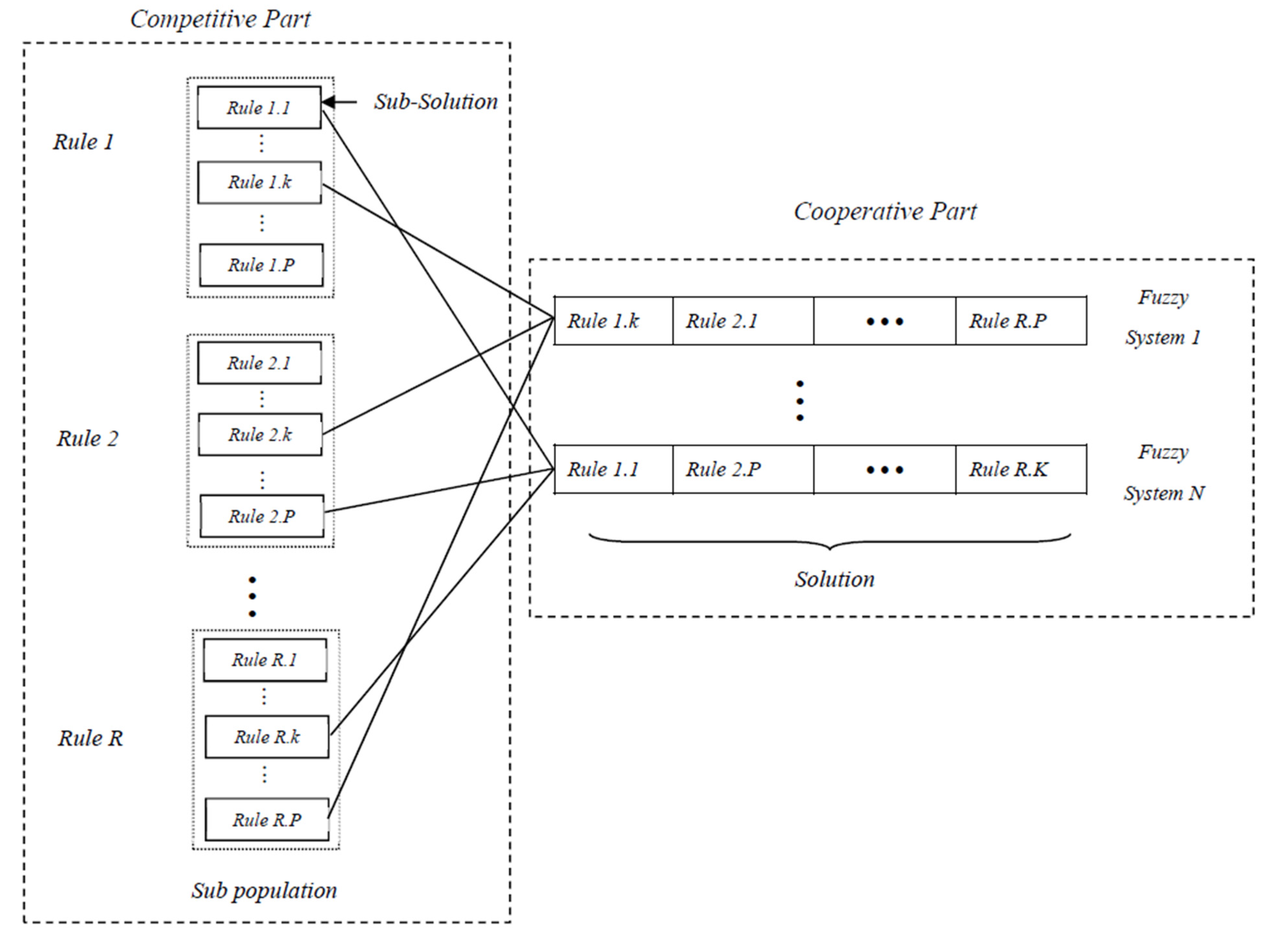
- The cooperative-competitive learning (CCL) approach, in which the chromosomes compete and cooperate simultaneously [58,59,60,61]. This can be understood in two opposite ways: the individuals could collaborate for the same purpose and thus construct the solution together, or they could compete against each other for the same resources. The use of CCL algorithms is recommended when the following issues arise: the search space is huge, the problem may be decomposed into subcomponents or different coding schemes are used [62].
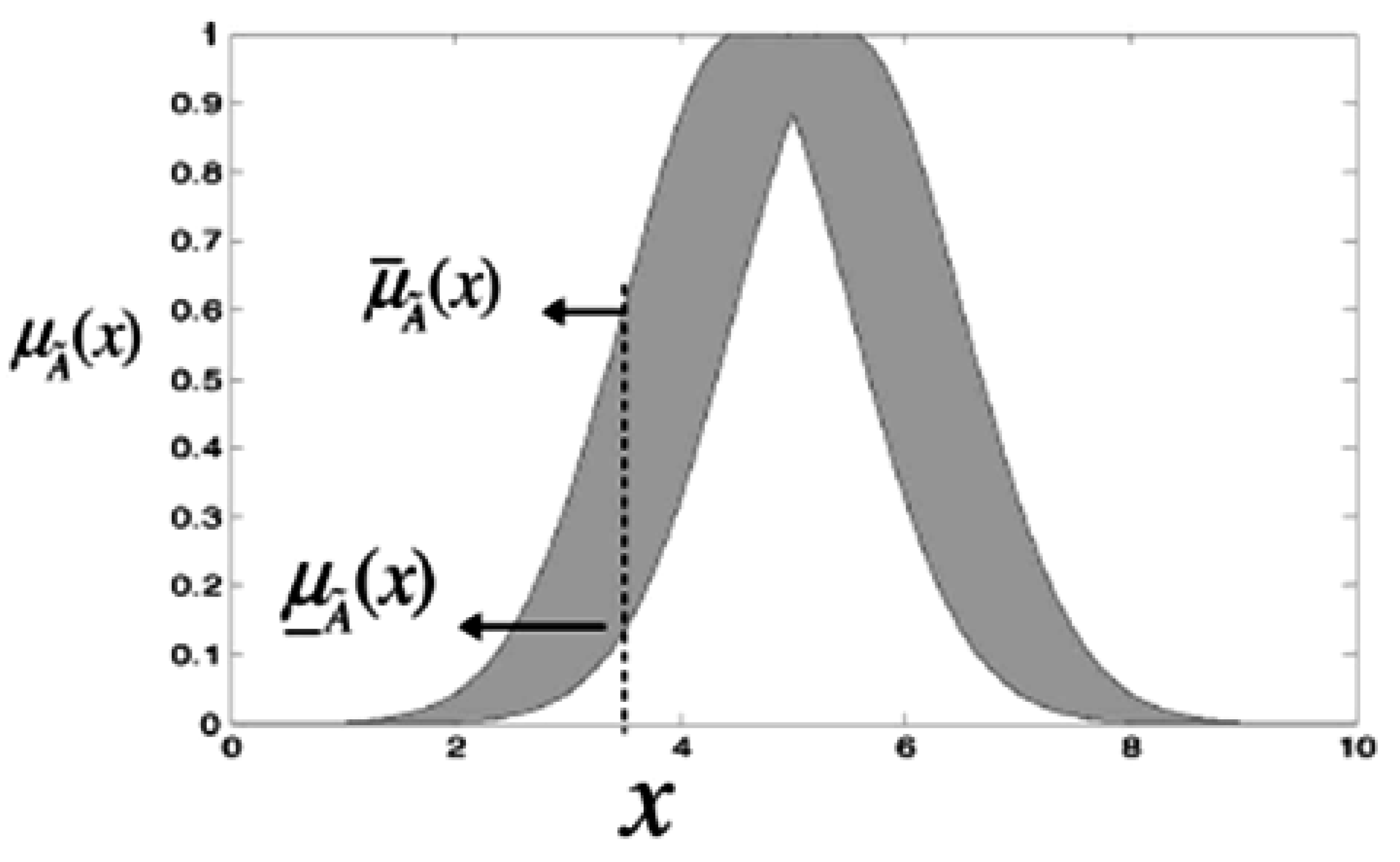
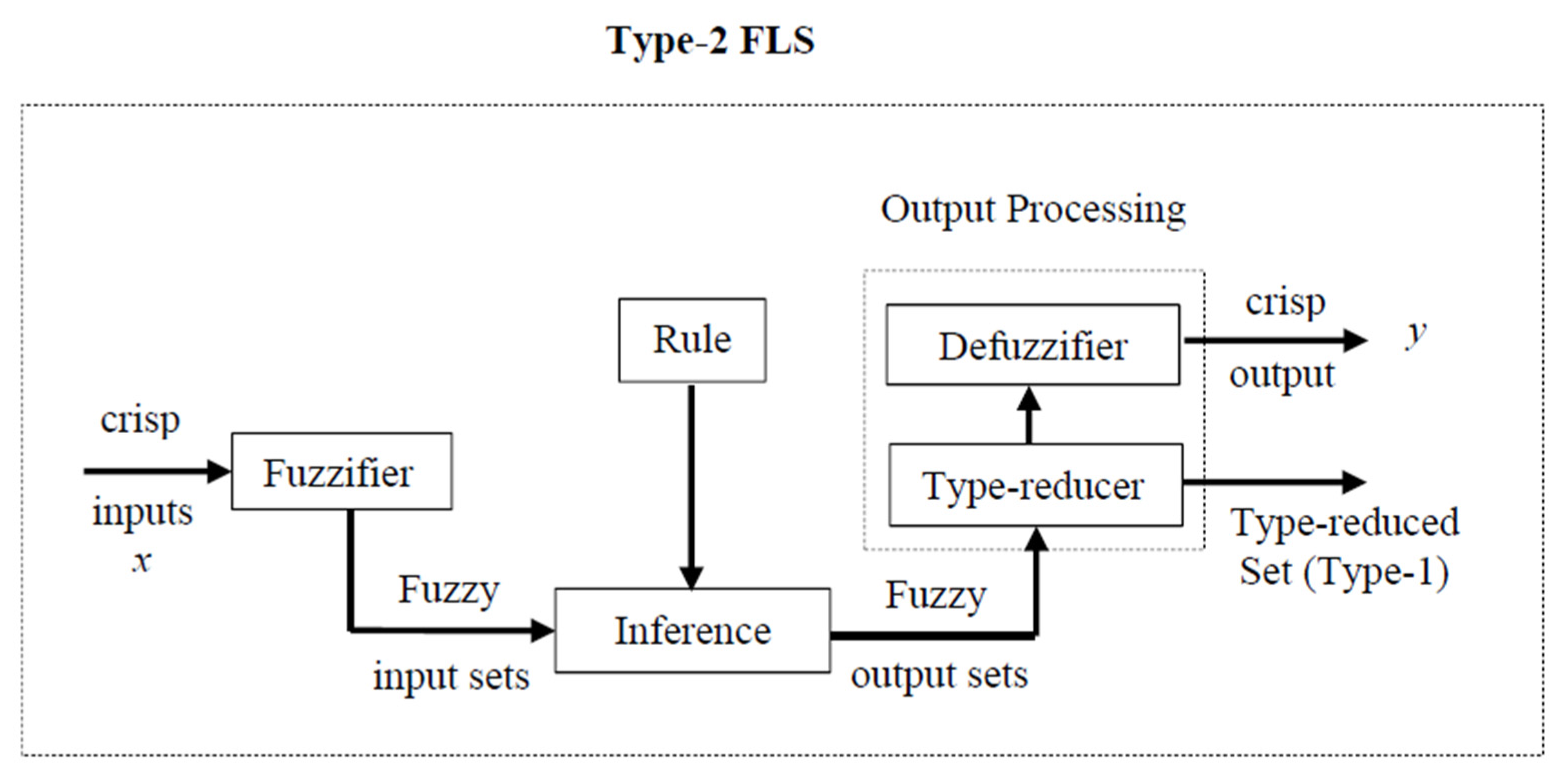
3. Type-2 Fuzzy Logic System (T2 FLS)


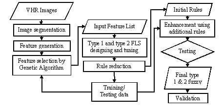
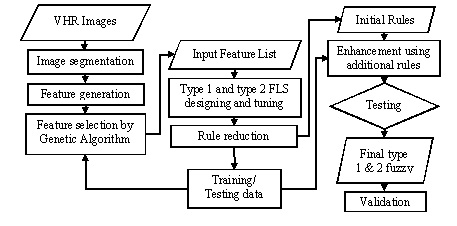
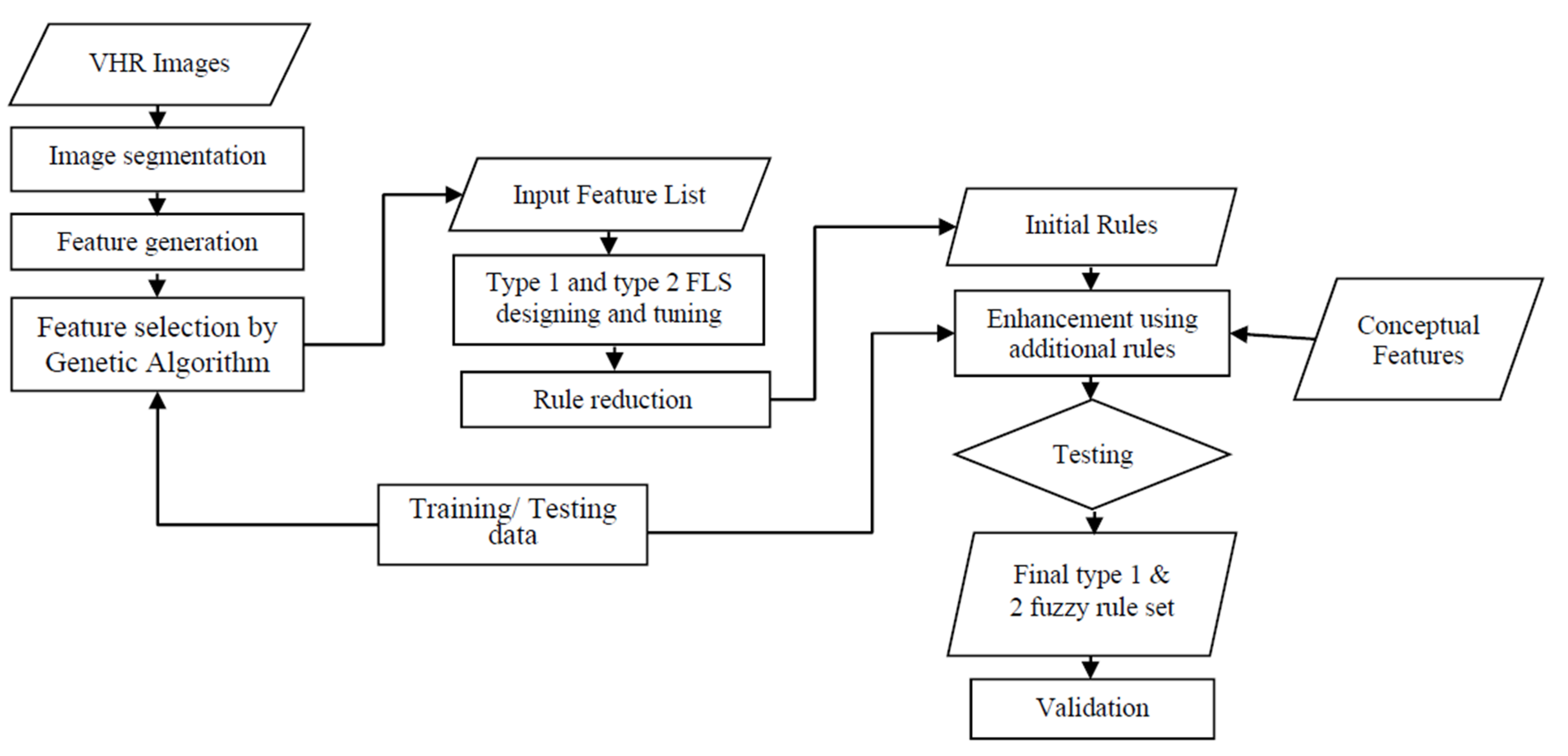
4. Proposed Method

4.1. Object-Based Feature Generation
4.2. Feature Selection by the GA
4.3. Designing and Tuning the FLSs
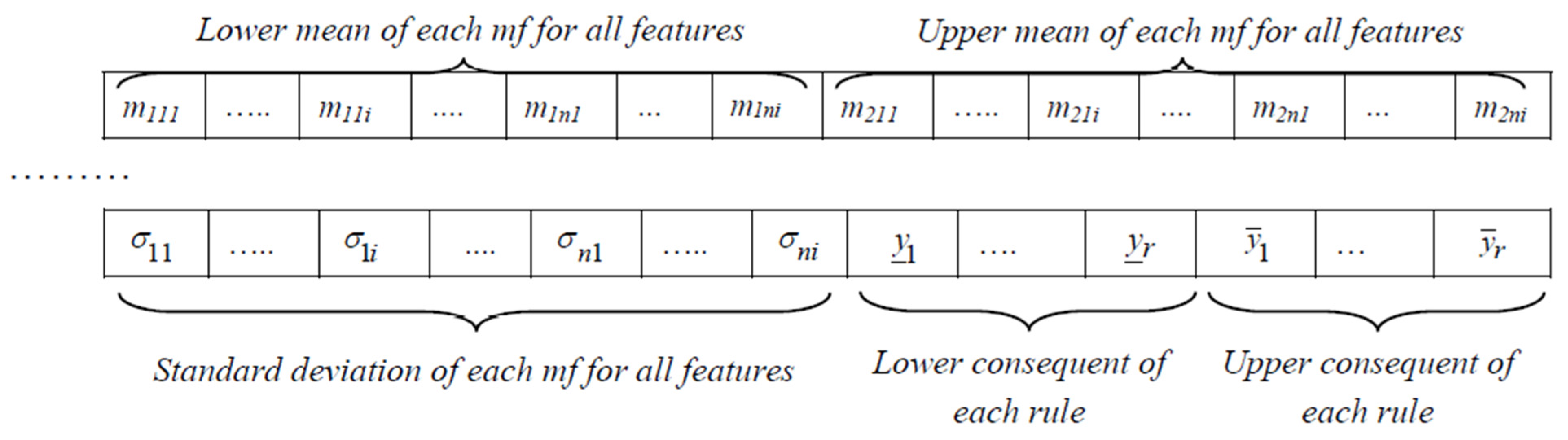
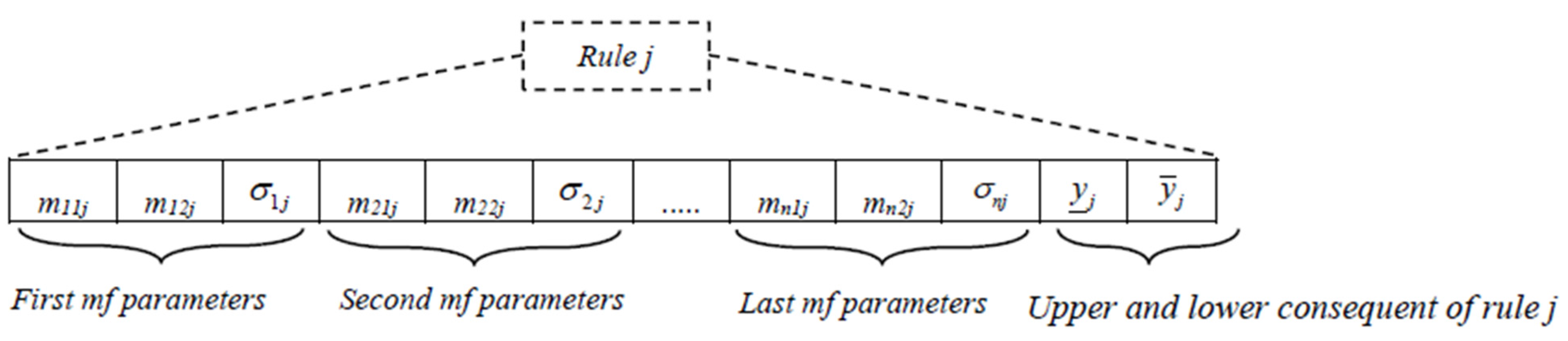
4.3.1. Initial Population Production


4.3.2. Fitness Function
4.3.3. Reproduction, Crossover and Mutation
4.4. Rule Reduction
4.5. Testing and Enhancement
4.6. Validation
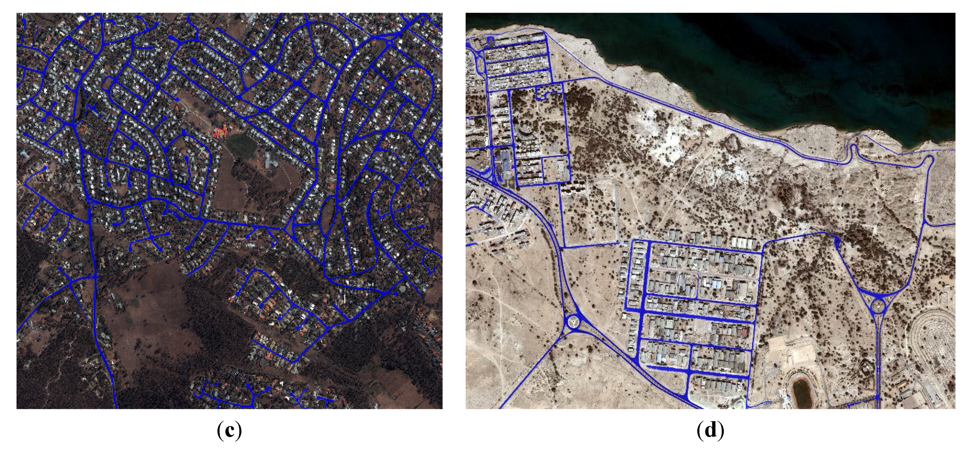
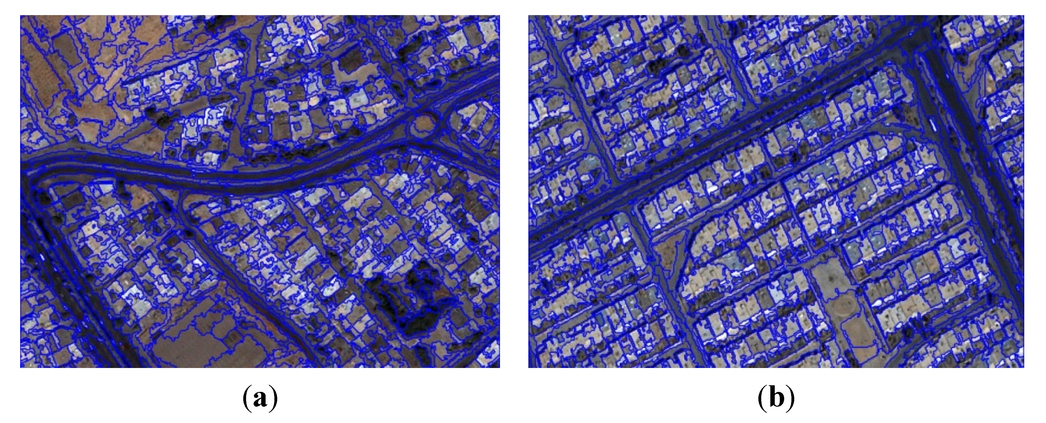
5. Implementation and Analysis
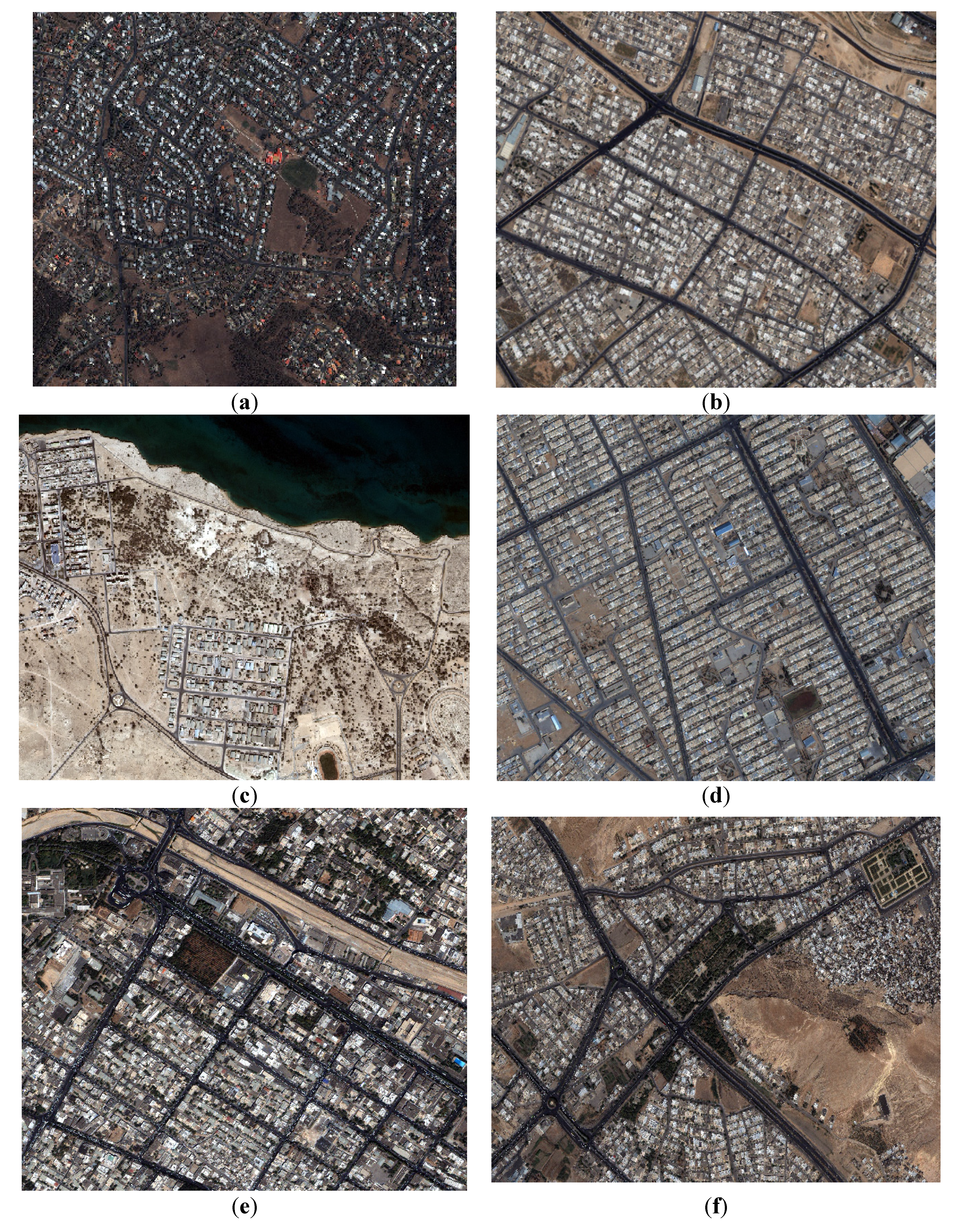
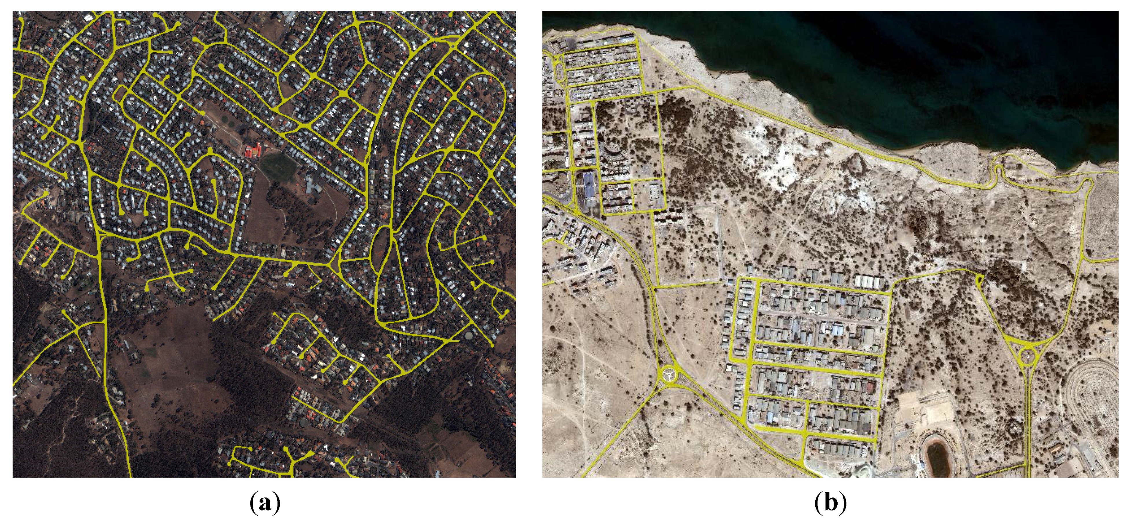
5.1. Input Data
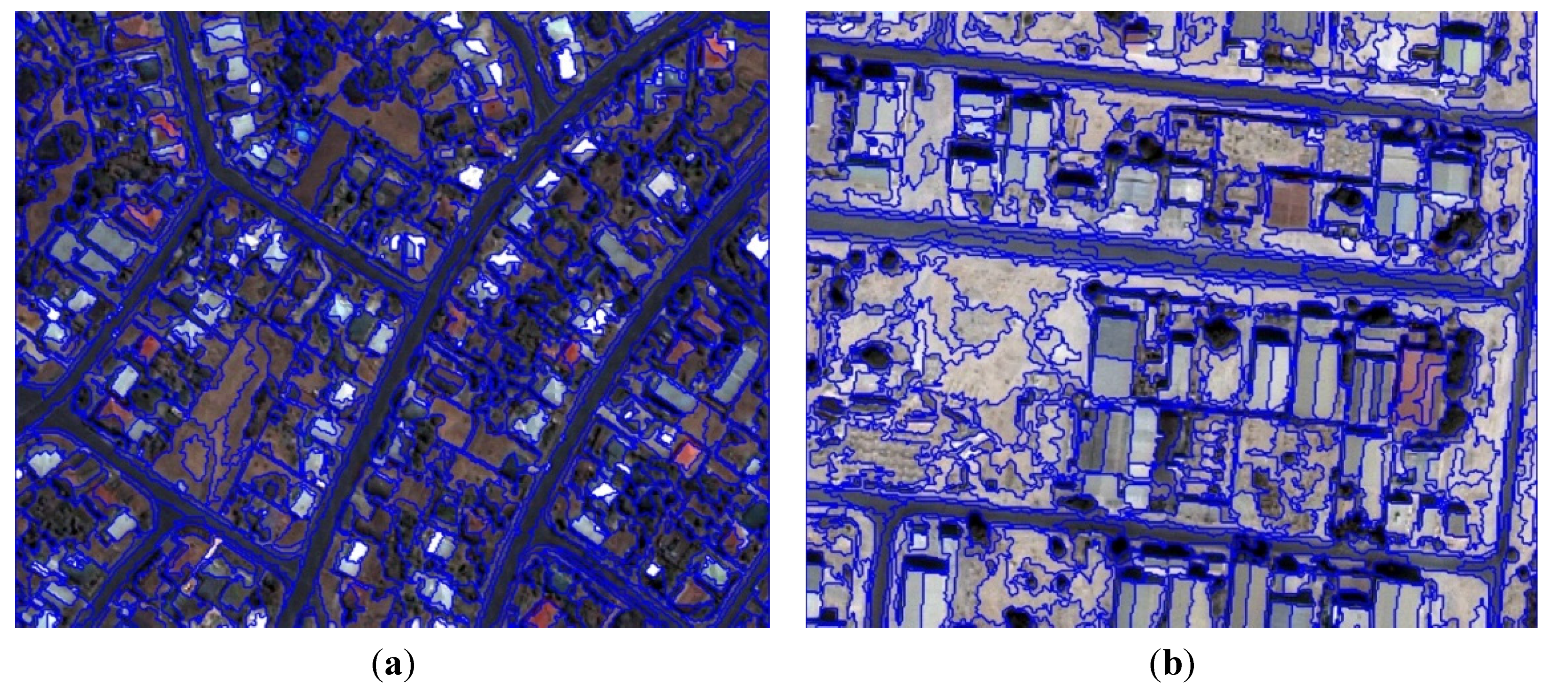
5.2. Object-Based Feature Selection


| Spectral | Shape | Texture | Combination |
|---|---|---|---|
| Mean (for 4 bands:NIR,Red,Green,Blue) | Area | GLCM homogeneity (for 4 bands in all.dir) | Intensity/Density |
| Brightness | Asymmetry | GLCM contrast (for 4 bands in all.dir) | Saturation/Density |
| Max. diff | Shape index | GLCM dissimilarity (for 4 bands in all.dir) | Intensity/compactness |
| Standard deviation (for 4 bands) | Roundness | GLCM entropy (for 4 bands in all.dir) | Saturation/shape Index |
| Ratio (for 4 bands) | Rectangular fit | GLCM mean (for 4 bands in all.dir) | Intensity/Shape Index |
| Contrast to neighbor (for 4 bands) | width | GLCM stddev (for 4 bands in all.dir) | Area × Max diff/ Border length |
| Std. deviation to neighbor (for 4 bands) | Border index | GLCM ang. 2nd moment (for 4 bands in all.dir) | Ratio Red/Density |
| Mean diff. to neighbors (for 4 bands) | length | Area × Ratio red/Border length | |
| Mean diff. to darker neighbors (for 4 bands) | Density | Hue/Density | |
| Mean diff. to brighter neighbors (for 4 bands) | Elliptic fit | Hue/Shape Index | |
| Hue | Compactness | Max diff/Density | |
| Intensity | Length/Width | Max diff/Rectangular Fit | |
| saturation | Border length | Max diff/Shape Index | |
| NDVI | Ratio Red/Rectangular Fit | ||
| NDWI | Ratio Red/Shape Index |
| NDVI | Standard deviation Blue | Hue | Brightness |
| NDWI | GLCM Homogeneity Blue | Ratio Red | Saturation/Density |
| Feature Description | |
|---|---|
| Brightness | Sum of the mean values of the layers containing spectral information divided by their quantity computed for an image object. |
| Standard deviation | Calculated from the layer values of all n pixels forming an image object. |
| Hue | The hue value of the HSI color space representing the gradation of color. |
| Saturation | The saturation value of the HSI color space representing the intensity of a specific hue. Relative purity of color; pure spectrum colors are fully saturated. |
| Ratio | The ratio of layer k reflects the amount that layer k contributes to the total brightness. |
| GLCM Homogeneity | It is a measure of the amount of local homogeneity in the image object. |
| NDVI | (NIR − Red) / (NIR + Red) |
| NDWI | (Green − NIR) / (Green + NIR) |
| Density | The density expressed by the area covered by the image object divided by its radius. |
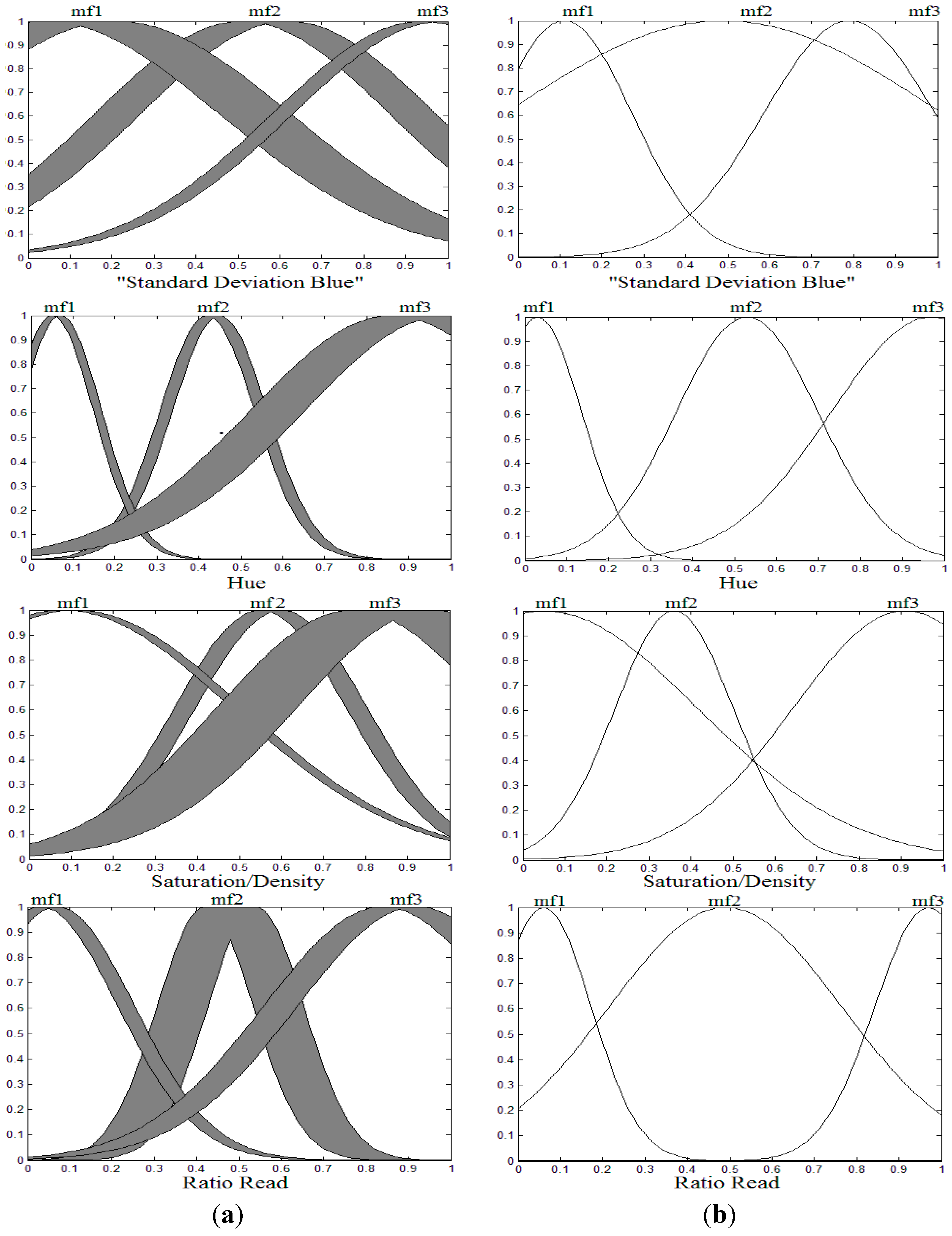
5.3. Type 2 FLS Designing and Tuning
| Accuracy | T2 FLS | T1 FLS | ||
|---|---|---|---|---|
| Road | Non Road | Road | Non Road | |
| Completeness | 0.97 | 0.9733 | 0.97 | 0.9667 |
| correctness | 0.9479 | 0.9848 | 0.9357 | 0.9848 |
| Kappa | 0.9379 | 0.9282 | ||

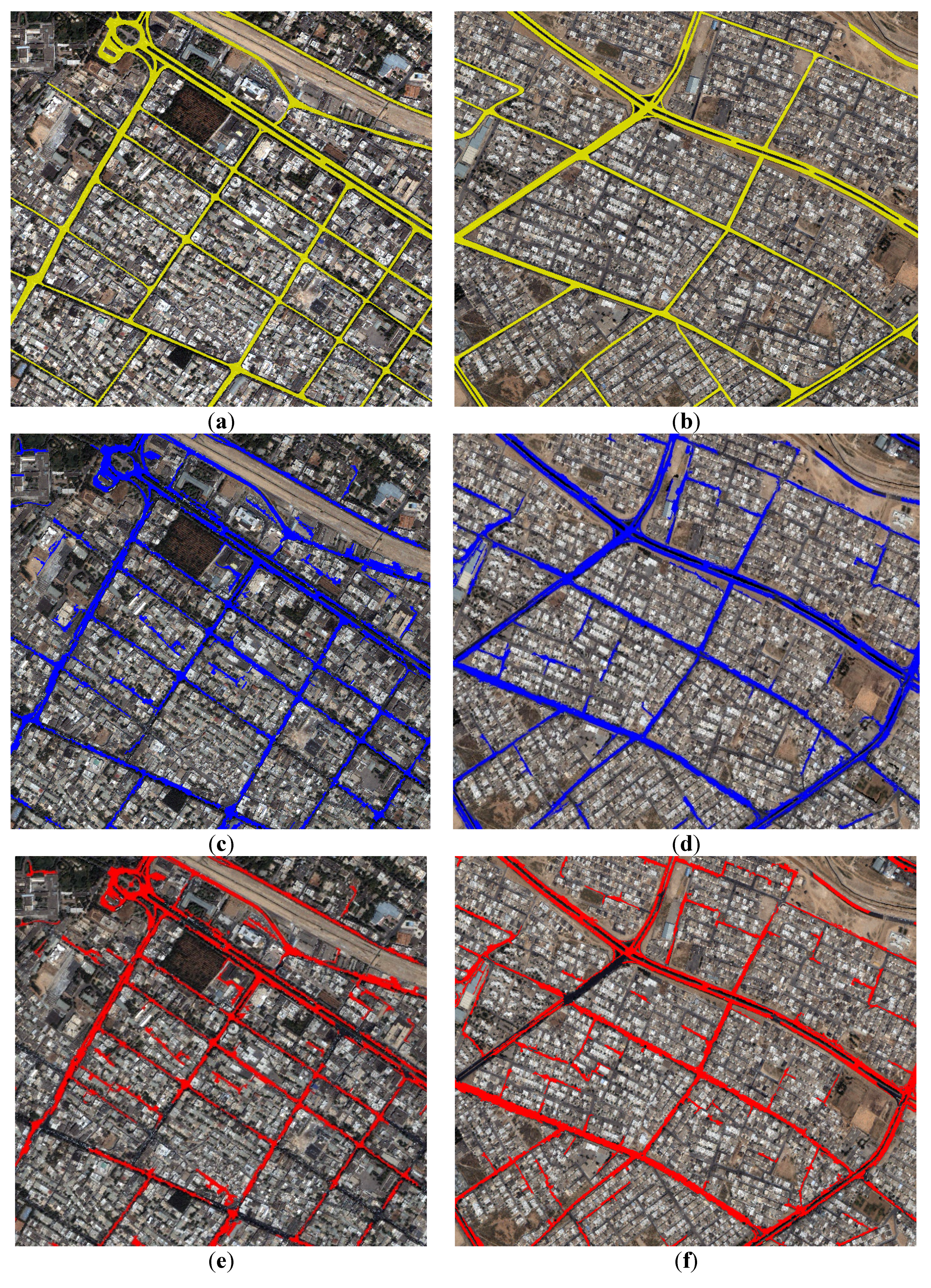
5.4. Testing and Enhancement
| Class | Test Images | T2 FLS | T1 FLS | |||||
|---|---|---|---|---|---|---|---|---|
| Completeness | Correctness | Kappa | Completeness | Correctness | Kappa | |||
| Road | Kish | 0.8577 | 0.7926 | 0.8173 | 0.8587 | 0.7526 | 0.7946 | |
| Hobart | 0.8897 | 0.8036 | 0.8323 | 0.8852 | 0.7773 | 0.8141 | ||
| Non Road | Kish | 0.9920 | 0.9949 | 0.8173 | 0.9899 | 0.9949 | 0.7946 | |
| Hobart | 0.9839 | 0.9918 | 0.8323 | 0.9812 | 0.9914 | 0.8141 | ||


| Class | Test Images | T2 FLS | T1 FLS | ||||
|---|---|---|---|---|---|---|---|
| Completeness | Correctness | Kappa | Completeness | Correctness | Kappa | ||
| Road | Kish | 0.8615 | 0.8433 | 0.8454 | 0.8635 | 0.8081 | 0.8273 |
| Hobart | 0.8933 | 0.8455 | 0.8581 | 0.8897 | 0.8272 | 0.8457 | |
| Non Road | Kish | 0.9943 | 0.9950 | 0.8454 | 0.9927 | 0.9951 | 0.8273 |
| Hobart | 0.9879 | 0.9921 | 0.8581 | 0.9862 | 0.9918 | 0.8457 | |
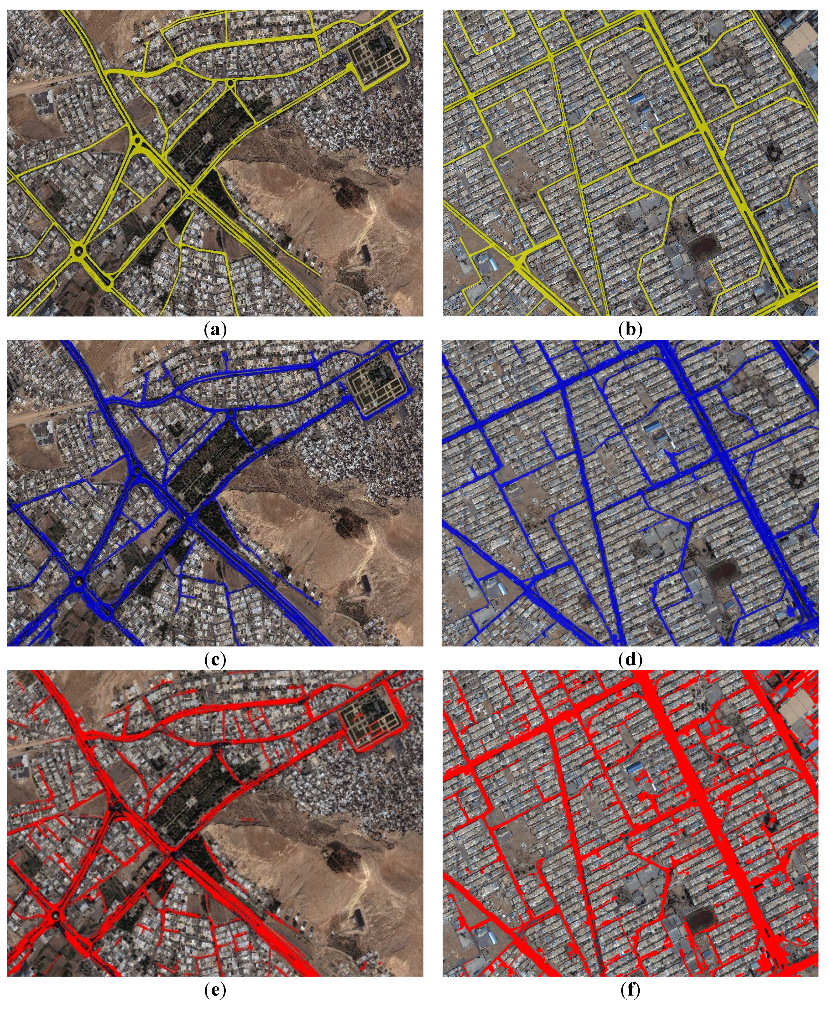
5.5. Validation

| Class | Validation Images | T2 FLS | T1 FLS | ||||
|---|---|---|---|---|---|---|---|
| Completeness | Correctness | Kappa | Completeness | Correctness | Kappa | ||
| Road | Shiraz | 0.8012 | 0.6961 | 0.7201 | 0.7840 | 0.5420 | 0.6018 |
| Yazd | 0.8433 | 0.6675 | 0.7138 | 0.8307 | 0.4863 | 0.5589 | |
| Hamadan1 | 0.7354 | 0.6801 | 0.6780 | 0.6561 | 0.6589 | 0.6255 | |
| Hamadan2 | 0.8084 | 0.6464 | 0.6922 | 0.7218 | 0.5736 | 0.6056 | |
| Non Road | Shiraz | 0.9683 | 0.9817 | 0.7201 | 0.9400 | 0.9796 | 0.6018 |
| Yazd | 0.9543 | 0.9825 | 0.7138 | 0.9046 | 0.9801 | 0.5589 | |
| Hamadan1 | 0.9676 | 0.9750 | 0.6780 | 0.9682 | 0.9678 | 0.6255 | |
| Hamadan2 | 0.9634 | 0.9838 | 0.6922 | 0.9556 | 0.9765 | 0.6056 | |


| Class | Validation images | T2 FLS | T1 FLS | |||||
|---|---|---|---|---|---|---|---|---|
| Completeness | Correctness | Kappa | Completeness | Correctness | Kappa | |||
| Road | Shiraz | 0.8034 | 0.7455 | 0.7520 | 0.7883 | 0.6167 | 0.6604 | |
| Yazd | 0.8559 | 0.7043 | 0.7453 | 0.8357 | 0.5309 | 0.6015 | ||
| Hamadan1 | 0.7406 | 0.7021 | 0.6939 | 0.6587 | 0.6870 | 0.6426 | ||
| Hamadan2 | 0.8192 | 0.6813 | 0.7206 | 0.7326 | 0.6307 | 0.6490 | ||
| Non Road | Shiraz | 0.9751 | 0.9821 | 0.7520 | 0.9556 | 0.9803 | 0.6604 | |
| Yazd | 0.9609 | 0.9840 | 0.7453 | 0.9197 | 0.9810 | 0.6015 | ||
| Hamadan1 | 0.9706 | 0.9756 | 0.6939 | 0.9719 | 0.9682 | 0.6426 | ||
| Hamadan2 | 0.9683 | 0.9848 | 0.7206 | 0.9645 | 0.9776 | 0.6490 | ||
6. Conclusions
Acknowledgments
Author Contributions
Conflicts of Interest
References
- Baatz, M.; Schäpe, A. Multiresolution segmentation: An optimization approach for high quality multi-scale image segmentation. In Angewandte Geographische Informationsverarbeitung XII; Strobl, J., Blaschke, T., Eds.; Wichmann-Verlag: Heidelberg, Germany, 2000; pp. 12–23. [Google Scholar]
- Herold, M.; Scepan, J.; Muller, A.; Gunter, S. Object-oriented mapping and analysis of urban landuse/cover using IKONOS data. In Proceedings of the 22nd EARSEL Symposium Geoinformation for European-Wide Integration, Prague, Czech Republic, 4–6 June 2002; pp. 531–538.
- Benz, U.; Hofmann, P.; Willhauck, G.; Lingenfelder, I.; Heynen, M. Multiresolution object-oriented fuzzy analysis of remote sensing data for GIS-ready information. ISPRS J. Photogramm. Remote Sens. 2004, 58, 239–258. [Google Scholar] [CrossRef]
- Mendel, J.M.; John, R.B. T2 fuzzy sets made simple. IEEE Trans. Fuzzy Syst. 2002, 10, 117–127. [Google Scholar] [CrossRef]
- Mena, J.B. State of the art on automatic road extraction for GIS update: A novel classification. Pattern Recognit. Lett. 2003, 24, 3037–3058. [Google Scholar] [CrossRef]
- Laptev, I.; Mayer, H.; Lindeberg, T.; Eckstein, W.; Steger, C.; Baumgartner, A. Automatic extraction of roads from aerial images based on scale-space and snakes. Mach. Vis. Appl. 2003, 12, 13–23. [Google Scholar] [CrossRef]
- Gruen, A.; Li, H. Semi-automatic linear feature extraction by dynamic programming and LSB snakes. Photogramm. Eng. Remote Sens. 1997, 63, 985–995. [Google Scholar]
- Doucette, P.; Agouris, P.; Stefanidis, A. Automated road extraction from high resolution multispectral imagery. Photogramm. Eng. Remote Sens. 2004, 70, 1405–1416. [Google Scholar] [CrossRef]
- Zhang, Q.; Couloigner, I. Wavelet approach to road extraction from high spatial resolution remotely sensed imagery. Geomatica 2004, 58, 33–39. [Google Scholar]
- Mokhtarzade, M.; Valadan Zoej, M.J. Road detection from high-resolution satellite images using artificial neural networks. Int. J. Appl. Earth Obs. Geoinf. 2007, 9, 32–40. [Google Scholar] [CrossRef]
- Peng, T. Incorporating generic and specific prior knowledge in a multiscale phase field model for road extraction from VHR Images. IEEE J. Sel. Top. Appl. Earth Obs. Remote Sens. 2008, 1, 130–148. [Google Scholar] [CrossRef] [Green Version]
- Valero, S.; Chanussot, J.; Benediktsson, J.A.; Talbot, H.; Waske, B. Advanced directional mathematical morphology for the detection of the road network in very high resolution remote sensing images. Pattern Recognit. Lett. 2010, 31, 1120–1127. [Google Scholar] [CrossRef] [Green Version]
- Movaghati, S.; Moghaddamjoo, A.; Tavakoli, A. Road extraction from satellite images using particle filtering and extended kalman filtering. IEEE Trans. Geosci. Remote Sens. 2010, 48, 2807–2815. [Google Scholar] [CrossRef]
- Mirnalinee, T.T.; Das, S.; Varghese, K. An integrated multistage framework for automatic road extraction from high resolution satellite imagery. J. Indian Soc. Remote Sens. 2011, 39, 1–25. [Google Scholar] [CrossRef]
- Shao, Y. Application of a fast linear feature detector to road extraction from remotely sensed imagery. IEEE J. Sel. Top. Appl. Earth Obs. Remote Sens. 2011, 4, 626–631. [Google Scholar] [CrossRef]
- Shi, W.; Miao, Z.; Debayle, J. An integrated method for urban main-road centerline extraction from optical remotely sensed imagery. IEEE Trans. Geosci. Remote Sens. 2014, 52, 3359–3372. [Google Scholar] [CrossRef]
- Miao, Z.; Wang, B.; Shi, B.; Wu, H. A method for accurate road centerline extraction from a classified image. IEEE J. Sel. Top. Appl. Earth Obs. Remote Sens. 2014, 7, 4762–4771. [Google Scholar] [CrossRef]
- Boyko, A.; Funkhouser, T. Extracting roads from dense point clouds in large scale urban environment. ISPRS J. Photogramm. Remote Sens. 2011, 66, s2–s12. [Google Scholar] [CrossRef]
- Yu, Y.; Li, J.; Guan, H.; Jia, F.; Wang, C. Learning hierarchical features for automated extraction of road markings from 3-D mobile LIDAR point clouds. IEEE J. Sel. Top. Appl. Earth Obs. Remote Sens. 2015, 8, 709–726. [Google Scholar] [CrossRef]
- He, C.; Yang, F.; Yin, S.; Deng, X.; Liao, M. Stereoscopic road network extraction by decision-level fusion of optical and SAR imagery. IEEE J. Sel. Top. Appl. Earth Obs. Remote Sens. 2013, 6, 2221–2228. [Google Scholar]
- Lu, P.; Du, K.; Yu, W.; Wang, R.; Deng, Y.; Balz, T. A new region growing-based method for road network extraction and its application on different resolution SAR images. IEEE J. Sel. Top. Appl. Earth Obs. Remote Sens. 2014, 7, 4772–4783. [Google Scholar] [CrossRef]
- Blaschke, T.; Strobl, J. What’s wrong with pixels? Some recent developments interfacing remote sensing and GIS. GeoBIT/GIS. 2001, 6, 12–17. [Google Scholar]
- Cleve, C.; Kelly, M.; Kearns, F.R.; Moritz, M. Classification of the wild land urban interface: A comparison of pixel- and object-based classifications using high resolution aerial photography. Comput. Environ. Urban Syst. 2008, 32, 317–326. [Google Scholar] [CrossRef]
- Blaschke, T. Object based image analysis for remote sensing. ISPRS J. Photogramm. Remote Sens. 2010, 65, 2–16. [Google Scholar] [CrossRef]
- Baltasavias, E. Object extraction and revision by image analysis using existing geo data and knowledge: Current status and steps towards operational systems. ISPRS J. Photogramm. Remote Sens. 2004, 58, 129–151. [Google Scholar] [CrossRef]
- Laliberte, A.S.; Rango, A.; Havstad, K.M.; Paris, J.F.; Beck, R.F.; McNeely, R.; Gonzalez, A.L. Object-oriented image analysis for mapping shrub encroachment from 1937 to 2003 in southern New Mexico. Remote Sens. Environ. 2004, 93, 198–210. [Google Scholar] [CrossRef]
- Frohn, R.C.; Hinkel, K.M.; Eisner, W.R. Satellite remote sensing classification of thaw lakes and drained thaw lake basins on the North Slope of Alaska. Remote Sens. Environ. 2005, 97, 116–126. [Google Scholar] [CrossRef]
- Ehlers, M.; Gähler, M.; Janowsky, R. Automated techniques for environmental monitoring and change analyses for ultra-high-resolution remote sensing data. Photogramm. Eng. Remote Sens. 2006, 72, 835–844. [Google Scholar] [CrossRef]
- Im, J.; Jensen, J.R.; Tullis, J.A. Object-based change detection using correlation image analysis and image segmentation. Int. J. Remote Sens. 2008, 29, 399–423. [Google Scholar] [CrossRef]
- Huang, X.; Zhang, L. An SVM ensemble approach combining spectral, structural, and semantic features for the classification of high-resolution remotely sensed imagery. IEEE Trans. Geosci. Remote Sens. 2013, 51, 257–272. [Google Scholar] [CrossRef]
- Huang, X.; Zhang, L. Road centreline extraction from high-resolution imagery based on multiscale structural features and support vector machines. Int. J. Remote Sens. 2009, 30, 1977–1987. [Google Scholar] [CrossRef]
- Zarrinpanjeh, N.; Samadzadegan, F.; Schenk, T. A new ant based distributed framework for urban road map updating from high resolution satellite imagery. Comput. Geosci. 2013, 54, 337–350. [Google Scholar] [CrossRef]
- Grote, A.; Heipke, C.; Rottensteiner, F. Road network extraction in suburban areas. Photogramm. Rec. 2012, 27, 8–28. [Google Scholar] [CrossRef]
- Agouris, P.; Gyftakis, S.; Stefanidis, A. Using a fuzzy supervisor for object extraction within an integrated geospatial environment. Int. Arch. Photogramm. Remote Sens. Spat. Inf. Sci. 1998, 32, 191–195. [Google Scholar]
- Amini, J.; Lucas, C.; Saradjian, M.R.; Azizi, A.; Sadeghian, S. Fuzzy logic system for road identification using IKONOS images. Photogramm. Rec. 2002, 17, 493–503. [Google Scholar] [CrossRef]
- Hinz, S.; Wiedemann, C. Increasing efficiency of road extraction by self-diagnosis. Photogramm. Eng. Remote Sens. 2004, 70, 1457–1466. [Google Scholar] [CrossRef]
- Bacher, U.; Mayer, H. Automatic road extraction from multispectral high resolution satellite images. Int. Arch. Photogramm. Remote Sens. Spat. Inf. Sci. 2005, 36, Part 3/W24. 29–34. [Google Scholar]
- Mayer, H.; Hinz, S.; Bacher, U.; Baltsavias, E. A test of automatic road extraction approaches. Int. Arch. Photogramm. Remote Sens. Spat. Inf. Sci. 2006, 36, 209–214. [Google Scholar]
- Mohammadzadeh, A.; Tavakoli, A.; Valadan Zoej, M.J. Road extraction based on fuzzy logic and mathematical morphology from pan-sharpened IKONOS images. Photogramm. Rec. 2006, 21, 44–60. [Google Scholar] [CrossRef]
- Singh, P.P.; Garg, R.D. A two-stage framework for road extraction from high-resolution satellite images by using prominent features of impervious surfaces. Int. J. Remote Sens. 2014, 35, 8074–8107. [Google Scholar] [CrossRef]
- Melin, P.; Castillo, O. Hybrid Intelligent Systems for Pattern Recognition Using Soft Computing; Springer-Verlag: Berlin, Germany, 2005. [Google Scholar]
- Cordón, O.; Herrera, F.; Hoffmann, F.; Magdalena, L. Genetic Fuzzy Systems: Evolutionary Tuning and Learning of Fuzzy Knowledge Bases; World Scientific: Singapore, 2001; Chapters 1–5; pp. 1–350. [Google Scholar]
- Lopez, M.; Melin, P.; Castillo, O. Optimization of response integration with fuzzy logic in ensemble neural networks using genetic algorithms. Stud. Comput. Intell. 2008, 154, 129–150. [Google Scholar]
- Sanchez, D.; Melin, P. Modular neural network with fuzzy integration and its optimization using genetic algorithms for human recognition based on iris, ear and voice biometrics. In Soft Computing for Recognition Based on Biometrics; Studies in Computational Intelligence; Springer: Berlin/Heidelberg, Germany, 2010; Volume 312, pp. 85–102. [Google Scholar]
- Hidalgo, D.; Castillo, O.; Melin, P. T1 and T2 fuzzy inference systems as integration methods in modular neural networks for multimodal biometry and its optimization with genetic algorithms. Inf. Sci. 2009, 179, 2123–2145. [Google Scholar] [CrossRef]
- Wu, D.; Tan, W.W. Genetic learning and performance evaluation of interval T2 fuzzy logic controllers. Eng. Appl. Artif. Intell. 2006, 19, 829–841. [Google Scholar] [CrossRef]
- Cordón, O.; Gomide, F.; Herrera, F.; Hoffmann, F.; Magdalena, L. Ten years of genetic fuzzy systems: Current framework and new trend. Fuzzy Sets Syst. 2004, 141, 5–31. [Google Scholar] [CrossRef]
- Cordón, O. A historical review of evolutionary learning methods for Mamdani-type fuzzy rule-based systems: Designing interpretable genetic fuzzy systems. Int. J. Approx. Reason. 2011, 52, 894–913. [Google Scholar] [CrossRef]
- Castillo, O.; Melin, P. Optimization of T2 fuzzy systems based on bio-inspired methods: A concise review. Inf. Sci. 2012, 205, 1–19. [Google Scholar] [CrossRef]
- Papadakis, S.E.; Theocharis, J.B. A GA-based fuzzy modeling approach for generating TSK models. Fuzzy Sets Syst. 2002, 131, 121–152. [Google Scholar] [CrossRef]
- Casillas, J.; Martínez, P.; Benítez, A.D. Learning consistent, complete and compact sets of fuzzy rules in conjunctive normal form for regression problems. Soft Comput. 2009, 13, 451–465. [Google Scholar] [CrossRef]
- Sanza, J.; Fernández, A.; Bustince, H.; Herrerac, F. A genetic tuning to improve the performance of fuzzy rule-based classification systems with interval-valued fuzzy sets: Degree of ignorance and lateral position. Int. J. Approx. Reason. 2011, 52, 751–766. [Google Scholar] [CrossRef]
- Ishibuchi, H.; Nakashima, T.; Murata, T. Performance evaluation of fuzzy classifier systems for multidimensional pattern classification problems. IEEE Trans. Syst. Man Cybern. 1999, 29, 601–618. [Google Scholar] [CrossRef] [PubMed]
- Gonzblez, A.; Pérez, R. SLAVE: A genetic learning system based on an iterative approach. IEEE Trans. Fuzzy Syst. 1999, 7, 176–191. [Google Scholar] [CrossRef]
- González, A.; Herrera, F. Multi-stage genetic fuzzy systems based on the iterative rule learning approach. Mathw. Soft Comput. 1997, 4, 233–249. [Google Scholar]
- Cordón, O.; Del Jesús, M.J.; Herrera, F.; Lozano, M. MOGUL: A methodology to obtain genetic fuzzy rule-based systems under the iterative rule learning approach. Intell. Syst. 1999, 14, 1123–1153. [Google Scholar] [CrossRef]
- Stavrakoudis, D.G.; Theocharis, J.B.; Zalidis, G.C. A multistage genetic fuzzy classifier for land cover classification from satellite imagery. Soft Comput. 2011, 15, 2355–2374. [Google Scholar] [CrossRef]
- Palacios, A.M.; Sánchez, L.; Couso, I. Extending a simple genetic cooperative-competitive learning fuzzy classifier to low quality datasets. Evol. Intell. 2009, 2, 73–84. [Google Scholar] [CrossRef]
- Dorronsoro, B.; Danoy, G.; Nebro, A.J.; Bouvry, P. Achieving super-linear performance in parallel multi-objective evolutionary algorithms by means of cooperative coevolution. Comput. Oper. Res. 2013, 40, 1552–1563. [Google Scholar] [CrossRef]
- Wang, X.; Cheng, H.; Huang, M. QoS multicast routing protocol oriented to cognitive network using competitive coevolutionary algorithm. Expert Syst. Appl. 2014, 41, 4513–4528. [Google Scholar] [CrossRef]
- Chandra, R.; Frean, M.; Zhang, M. Crossover-based local search in cooperative co-evolutionary feedforward neural networks. Appl. Soft Comput. 2012, 12, 2924–2932. [Google Scholar] [CrossRef]
- Pena-Reyes, C.A. Fuzzy CoCo: A cooperative-coevolutionary approach to fuzzy modeling. IEEE Trans. Fuzzy Syst. 2001, 9, 727–737. [Google Scholar] [CrossRef]
- Zadeh, L.A. Fuzzy logic and approximate reasoning. Syntheses 1975, 30, 407–428. [Google Scholar] [CrossRef]
- Mizumoto, M.; Tanaka, K. Some properties of fuzzy sets of type 2. Inf. Control 1976, 31, 312–340. [Google Scholar] [CrossRef]
- Mizumoto, M.; Tanaka, K. Fuzzy sets and their operations. Inf. Control 1981, 48, 30–48. [Google Scholar] [CrossRef]
- Castillo, O.; Melin, P. T2 Fuzzy Logic: Theory and Applications; Springer-Verlag: Berlin, Germany, 2008. [Google Scholar]
- Melin, P.; Castillo, O. A review on the applications of T2 fuzzy logic in classification and pattern recognition. Expert Syst. Appl. 2013, 40, 5413–5423. [Google Scholar] [CrossRef]
- Karnik, N.N.; Mendel, J.M.; Liang, Q. T2 fuzzy logic systems. IEEE Trans. Fuzzy Syst. 1999, 7, 643–658. [Google Scholar] [CrossRef]
- Karnik, N.N.; Mendel, J.M. Operations on T2 fuzzy sets. Fuzzy Sets Syst. 2001, 122, 327–348. [Google Scholar] [CrossRef]
- Karnik, N.N.; Mendel, J.M. Centroid of a T2 fuzzy set. Inf. Sci. 2001, 132, 195–220. [Google Scholar] [CrossRef]
- Mendel, J. Uncertain Rule-Based Fuzzy Logic Systems: Introduction and Directions; University of Southern California: Los Angeles, CA, USA, 2000; Chapters 7–10; pp. 213–350. [Google Scholar]
- Mallinis, G.; Koutsias, N.; Tsakiri-Strati, M.; Karteris, M. Object-based classification using Quickbird imagery for delineating forest vegetation polygons in a Mediterranean test site. ISPRS J. Photogramm. Remote Sens. 2008, 63, 237–250. [Google Scholar] [CrossRef]
- Dragut, L.; Eisank, C. Automated object-based classification of topography from SRTM data. Geomorphology 2012, 141–142, 21–33. [Google Scholar] [CrossRef] [PubMed]
- Schneevoigt, N.J.; Linden, S.V.D.; Thamm, H.-P.; Schrott, L. Detecting alpine landforms from remotely sensed imagery: A pilot study in the Bavarian Alps. Geomorphology 2008, 93, 104–119. [Google Scholar] [CrossRef]
- Lucas, R.; Rowlands, A.; Brown, A.; Keyworth, S.; Bunting, P. Rule-based classification of multi-temporal satellite imagery for habitat and agricultural land cover mapping. ISPRS J. Photogramm. Remote Sens. 2007, 62, 165–185. [Google Scholar] [CrossRef]
- Gamanya, R.; Maeyer, P.D.; Dapper, M.D. An automated satellite image classification design using object-oriented segmentation algorithms: A move towards standardization. Expert Syst. Appl. 2007, 32, 616–624. [Google Scholar] [CrossRef]
- Stavrakoudis, D.G.; Theocharis, J.B.; Zalidis, G.C. A boosted genetic fuzzy classifier for land cover classification of remote sensing imagery. ISPRS J. Photogramm. Remote Sens. 2011, 66, 529–544. [Google Scholar] [CrossRef]
- Tseng, M.H.; Chen, S.J.; Hwang, G.H.; Shen, M.Y. A genetic algorithm rule-based approach for land-cover classification. ISPRS J. Photogramm. Remote Sens. 2008, 63, 202–212. [Google Scholar] [CrossRef]
- Wen, X.; Zhang, H.; Zhang, J.; Jiao, X.; Wang, L. Multiscale modeling for classification of SAR imagery using hybrid EM algorithm and genetic algorithm. Prog. Nat. Sci. 2009, 19, 1033–1036. [Google Scholar] [CrossRef]
- Nikfar, M.; Valadan Zoej, M.J.; Mohammadzadeh, A.; Mokhtarzade, M.; Navabi, A. Optimization of multiresolution segmentation by using a genetic algorithm. J. Appl. Remote Sens. 2012, 6, 1–18. [Google Scholar] [CrossRef]
- Li, S.; Wu, H.; Wan, A.; Zhu, J. An effective feature selection method for hyperspectral image classification based on genetic algorithm and support vector machine. Knowl.-Based Syst. 2011, 24, 40–48. [Google Scholar] [CrossRef]
- Puig, D.; Garcia, M.A. Automatic texture feature selection for image pixel classification. Pattern Recognit. 2009, 39, 1996–2009. [Google Scholar] [CrossRef]
- Krawiec, K.; Bhanu, B. Visual learning by coevolution feature synthesis. IEEE Trans. Syst. Man Cybern. 2005, 35, 409–425. [Google Scholar] [CrossRef]
- Chang, C.H.; Liu, C.C.; Wen, C.G. Integrating semi analytical and genetic algorithms to retrieve the constituents of water bodies from remote sensing of ocean color. Opt. Express 2007, 15, 252–265. [Google Scholar] [CrossRef] [PubMed]
- Ines, A.V.; Honda, K. On quantifying agricultural and water management practices from low spatial resolution RS data using genetic algorithms: A numerical study for mixed-pixel environment. Adv. Water Resour. 2005, 28, 856–870. [Google Scholar] [CrossRef]
- Holland, J. Adaptation in Natural and Artificial Systems; University of Michigan Press: Oxford, UK, 1975; pp. 62–143. [Google Scholar]
- Yu, C.; Cui, B.; Wang, S.; Su, J. Efficient index-based KNN join processing for high-dimensional data. Inf. Softw. Technol. 2007, 49, 332–334. [Google Scholar] [CrossRef]
- Chen, J.H. KNN based knowledge-sharing model for severe change order disputes in construction. Autom. Constr. 2008, 17, 773–779. [Google Scholar] [CrossRef]
- Saini, I.; Singh, D.; Khosla, A. QRS detection using K-Nearest Neighbor algorithm (KNN) and evaluation on standard ECG databases. J. Adv. Res. 2013, 4, 331–334. [Google Scholar] [CrossRef] [PubMed]
- Bishop, Y.M.M.; Fienberg, S.E.; Holland, P.W. Discrete Multivariate Analysis: Theory and Practice; MIT Press: Cambridge, MA, USA, 1975; pp. 105–171. [Google Scholar]
- Zhang, Y. Understanding image fusion. Photogramm. Eng. Remote Sens. 2004, 70, 657–661. [Google Scholar]
- Wiedemann, C.; Heipke, C.; Mayer, H.; Jamet, O. Empirical evaluation of automatically extracted road axes. In Empirical Evaluation Methods in Computer Vision; Bower, K.J., Philips, P.J., Eds.; IEEE Computer Society Press: Los Alamitos, CA, USA, 1998; pp. 172–187. [Google Scholar]
- Yang, Y.; Lohmann, P.; Heipke, C. Genetic algorithms for the unsupervised classification of satellite images. Int. Arch. Photogramm. Remote Sens. Spat. Inf. Sci. 2006, 36, 179–184. [Google Scholar]
- Hamedianfar, A.; Shafri, H.Z.M.; Mansor, S.; Ahmad, N. Improving detailed rule-based feature extraction of urban areas fromWorldView-2 image and LIDAR data. Int. J. Remote Sens. 2014, 35, 1876–1899. [Google Scholar] [CrossRef]
- Jin, X.; David, C.H. An integrated system for automatic road mapping from high-resolution multi-spectral satellite imagery by information fusion. Inf. Fusion 2005, 6, 257–273. [Google Scholar] [CrossRef]
© 2015 by the authors; licensee MDPI, Basel, Switzerland. This article is an open access article distributed under the terms and conditions of the Creative Commons Attribution license (http://creativecommons.org/licenses/by/4.0/).
Share and Cite
Nikfar, M.; Zoej, M.J.V.; Mokhtarzade, M.; Shoorehdeli, M.A. Designing a New Framework Using Type-2 FLS and Cooperative-Competitive Genetic Algorithms for Road Detection from IKONOS Satellite Imagery. Remote Sens. 2015, 7, 8271-8299. https://doi.org/10.3390/rs70708271
Nikfar M, Zoej MJV, Mokhtarzade M, Shoorehdeli MA. Designing a New Framework Using Type-2 FLS and Cooperative-Competitive Genetic Algorithms for Road Detection from IKONOS Satellite Imagery. Remote Sensing. 2015; 7(7):8271-8299. https://doi.org/10.3390/rs70708271
Chicago/Turabian StyleNikfar, Maryam, Mohammad Javad Valadan Zoej, Mehdi Mokhtarzade, and Mahdi Aliyari Shoorehdeli. 2015. "Designing a New Framework Using Type-2 FLS and Cooperative-Competitive Genetic Algorithms for Road Detection from IKONOS Satellite Imagery" Remote Sensing 7, no. 7: 8271-8299. https://doi.org/10.3390/rs70708271
APA StyleNikfar, M., Zoej, M. J. V., Mokhtarzade, M., & Shoorehdeli, M. A. (2015). Designing a New Framework Using Type-2 FLS and Cooperative-Competitive Genetic Algorithms for Road Detection from IKONOS Satellite Imagery. Remote Sensing, 7(7), 8271-8299. https://doi.org/10.3390/rs70708271