
Modeling Top of Atmosphere Radiance over Heterogeneous Non-Lambertian Rugged Terrain


Abstract
:
1. Introduction
2. Background

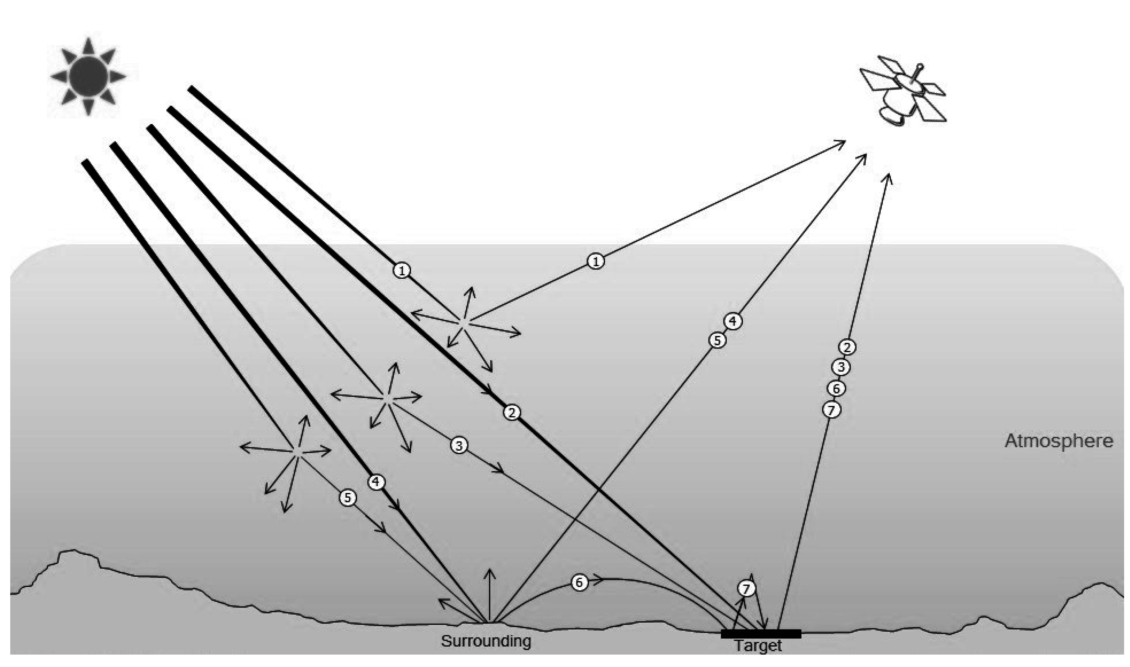
| Contribution in Figure 1 | Description | Corresponding Flux in Figure 2 |
|---|---|---|
| Contribution 1 | Spectral radiation originating from the sun and, after propagation in the atmosphere, scattered into the field of view of the sensor without reaching the surface. | |
| Contribution 2 | Direct radiation that goes through the atmosphere without being absorbed or scattered and after reflecting back from the surface it reaches the sensor. | integrated in |
| Contribution 3 | Spectral radiation scattered by the atmosphere onto the target and then reflected back towards the sensor. | integrated in |
| Contribution 4 and 5 | Spectral radiation that directly or diffusely reach the surrounding areas of the target and then reflected or scattered back into the field of view of the sensor. This effect is so called “adjacency effect” or “blurring effect”. | |
| Contribution 6 | Diffuse radiation coming from the adjacent features into the field of view of the sensor. This contribution is incorporated in Contribution 3. | - |
| Contribution 7 | So-called trapping effect and it is a part of the radiation reflected from the surface into the air column above the surface being scattered and ultimately reaches the sensor. This contribution is incorporated in Contribution 3. | - |

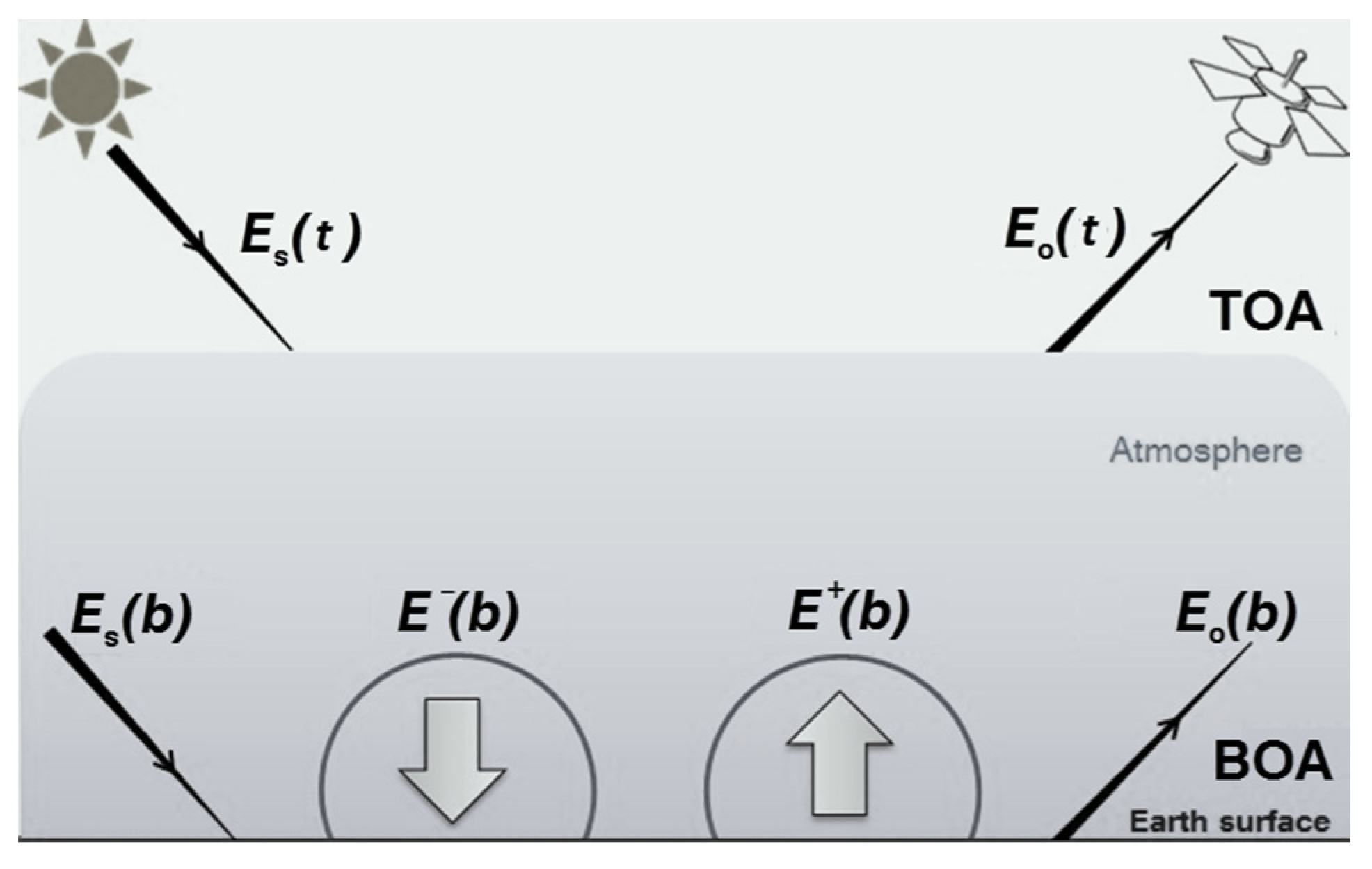
| Factor | Description | SI Unit |
|---|---|---|
| rso | surface bidirectional reflectance factor | - |
| surface hemispherical-directional reflectance for diffuse incidence | - | |
| spatially averaged directional-hemispherical reflectance over surroundings | - | |
| spatially averaged bi-hemispherical reflectance over surroundings | - | |
| TOA atmospheric bidirectional reflectance | - | |
| BOA spherical albedo of the atmosphere | - | |
| direct atmospheric transmittance from the sun to the ground | - | |
| direct atmospheric transmittance from the ground to the sensor | - | |
| diffuse atmospheric transmittance from the sun to the ground | - | |
| diffuse atmospheric transmittance from the ground to the sensor | - | |
| extraterrestrial solar irradiance on a plane perpendicular to the sunrays | Wm−2 | |
| direct solar irradiance on a horizontal plane | Wm−2µm−1 | |
| radiance in the viewing direction, times π | Wm−2µm−1 | |
| downward diffuse irradiance | Wm−2µm−1 | |
| upward diffuse irradiance | Wm−2µm−1 | |
| binary coefficient to indicate cast-shadowed pixels (0 or 1) | - | |
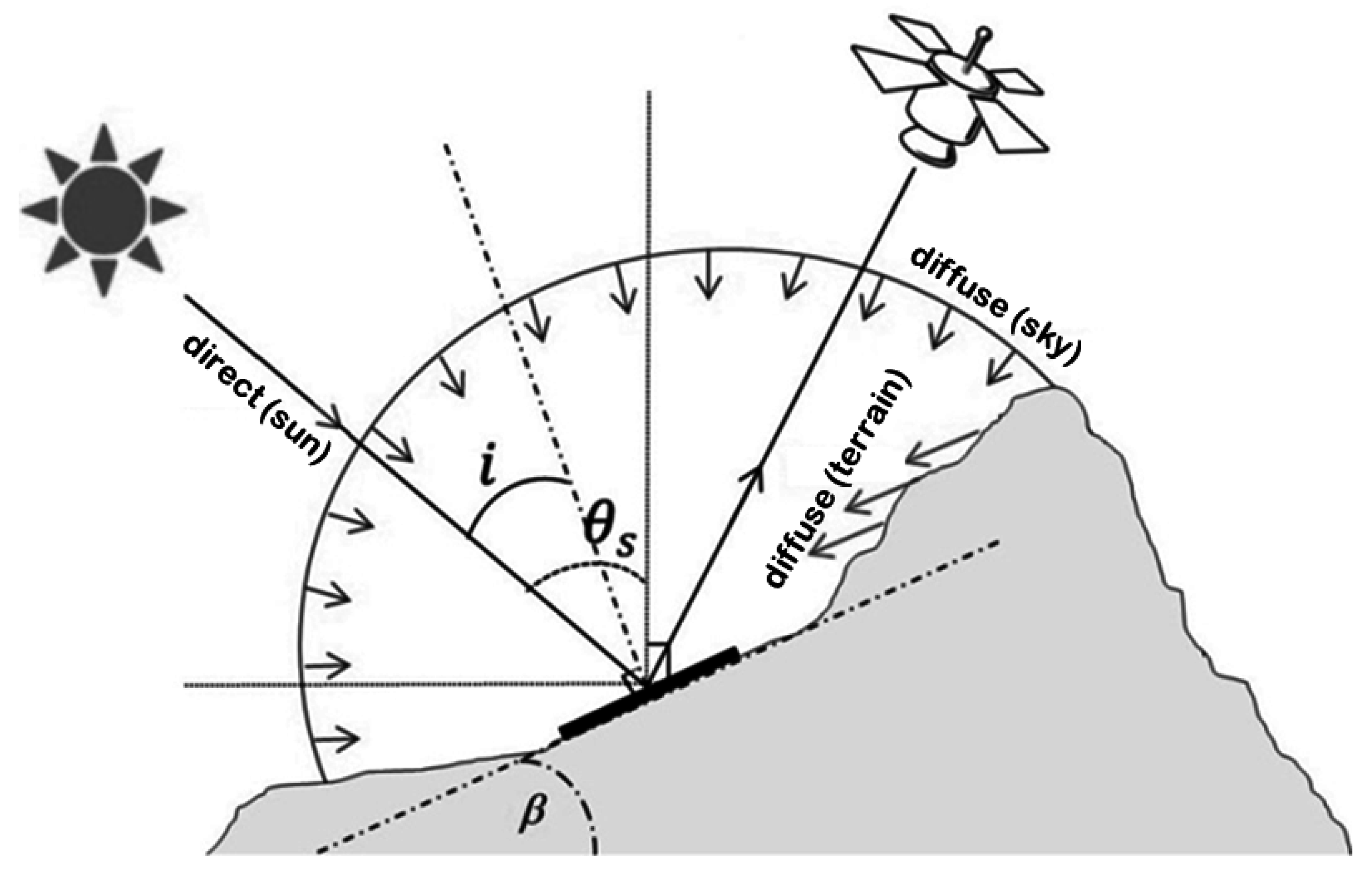
| local solar zenith angle | Degree | |
| viewing zenith angle | Degree | |
| angle between the surface normal and the sun ray (illumination angle) | Degree | |
| surface slope angle | Degree | |
| solar azimuth angle | Degree | |
| slope azimuth angle (aspect) | Degree | |
| indicates the quantity at the top of atmosphere | - | |
| indicates the quantity at the bottom of atmosphere | - |
3. Four-Stream Theory over Rugged Terrain
3.1. Irradiance Modeling

3.2. Reflectance Modeling
3.3. Top of Atmosphere Radiance over Rugged Terrain
3.4. Atmospheric Modeling
| MODTRAN (*.tp7 or *.7sc) | Column | Formula | Description |
|---|---|---|---|
| FREQ | 1 | - | band-center wavelength |
| TRAN | 2 | direct transmittance from the ground to the sensor | |
| PTH THRML | 3 | - | upwelling atmospheric emitted radiance received at the sensor (negligible in the reflective region) |
| THRML SCT | 4 | - | thermal scattering of the path radiance |
| SURF EMIS | 5 | - | surface emission received at the sensor |
| SOL SCAT | 6 | solar multi-scattered radiance received at the sensor(PATH) | |
| SING SCAT | 7 | - | solar single-scattered radiance |
| GRND RFLT | 8 | ground reflected radiance(GRT) | |
| DRCT RFLT | 9 | direct solar reflected radiance received at the sensor(GSUN) | |
| TOTAL RAD | 10 | TOTAL RAD = SOL SCAT + GRND RFLT | PTH THRML + SURF EMIS + SOL SCAT + GRND RFLT (GTOT) |
| REF SOL | 11 | SOL@OBS multiplied by | |
| SOL@OBS | 12 | extraterrestrial solar irradiance | |
| DEPTH | 13 | negative Log of the transmittance column TRAN (total optical thickness) |
4. Model Implementation
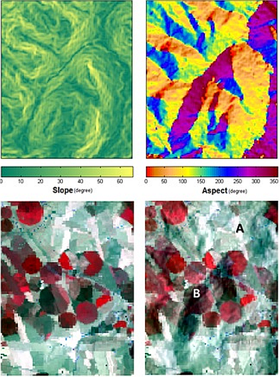
5. Design of the Numerical Experiment
6. Results and Discussion
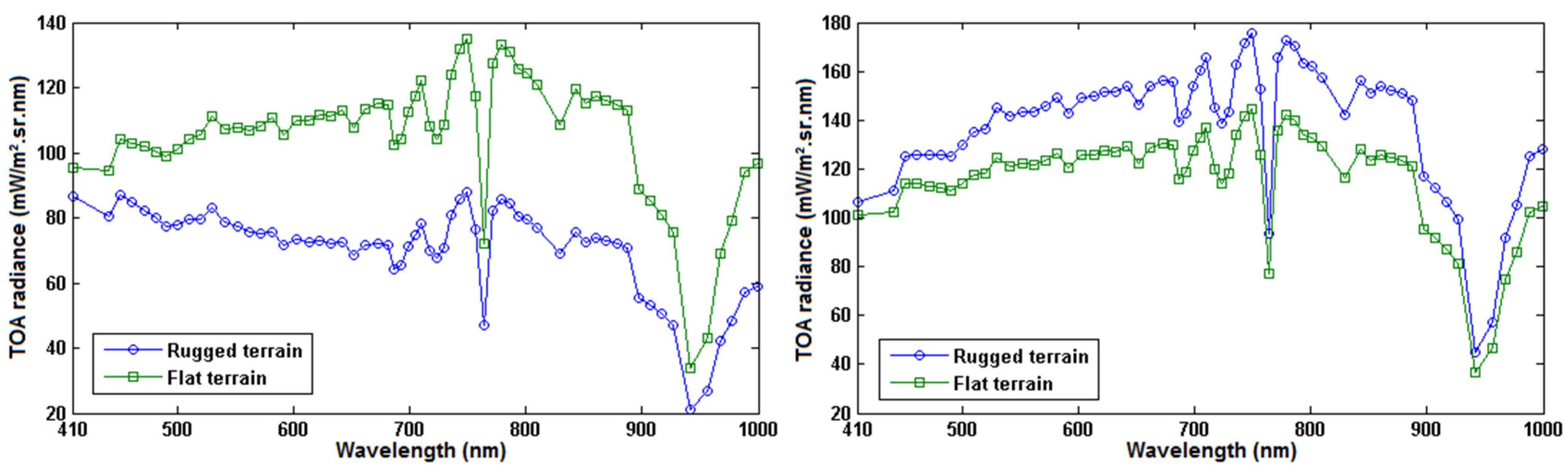
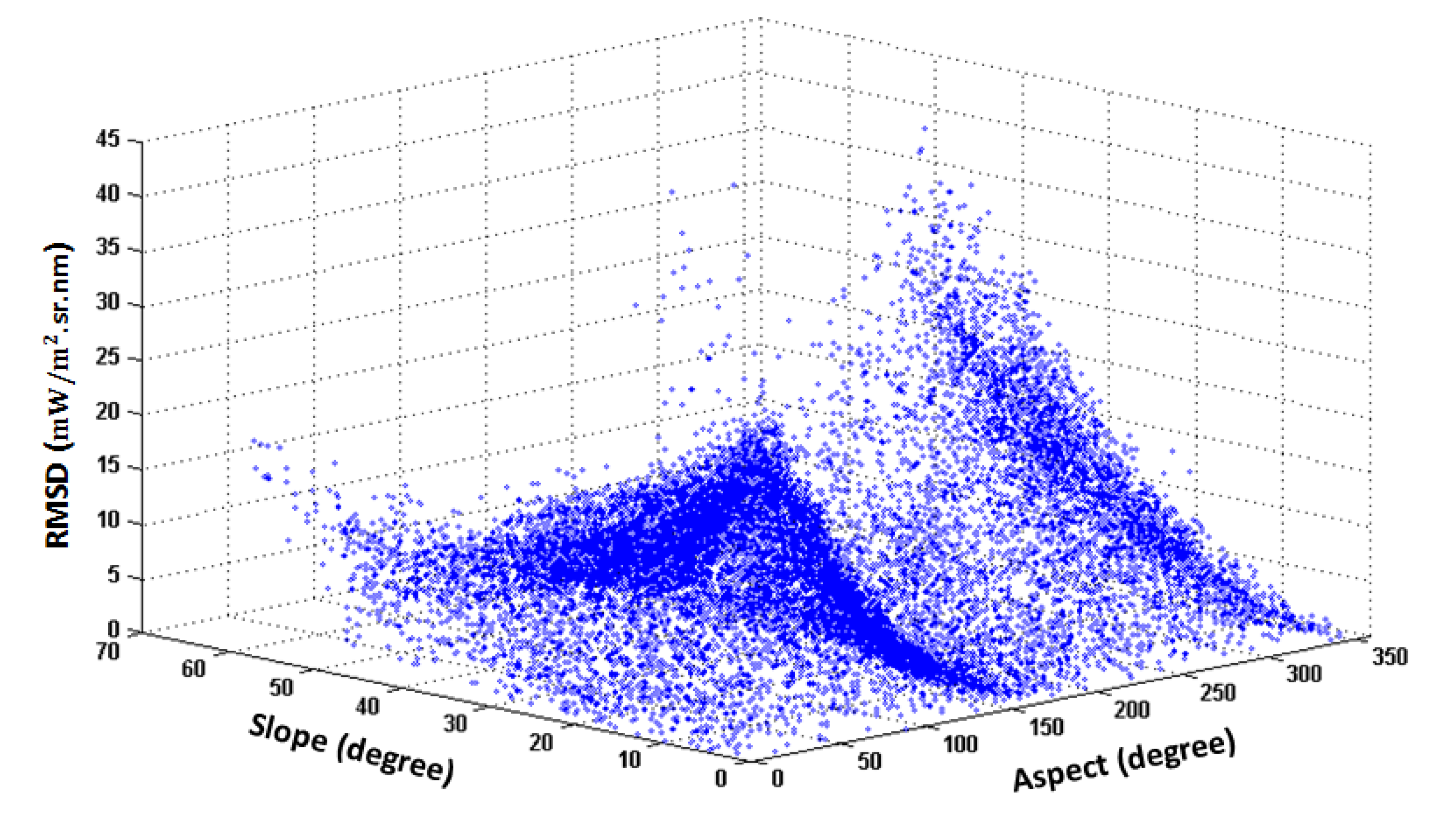
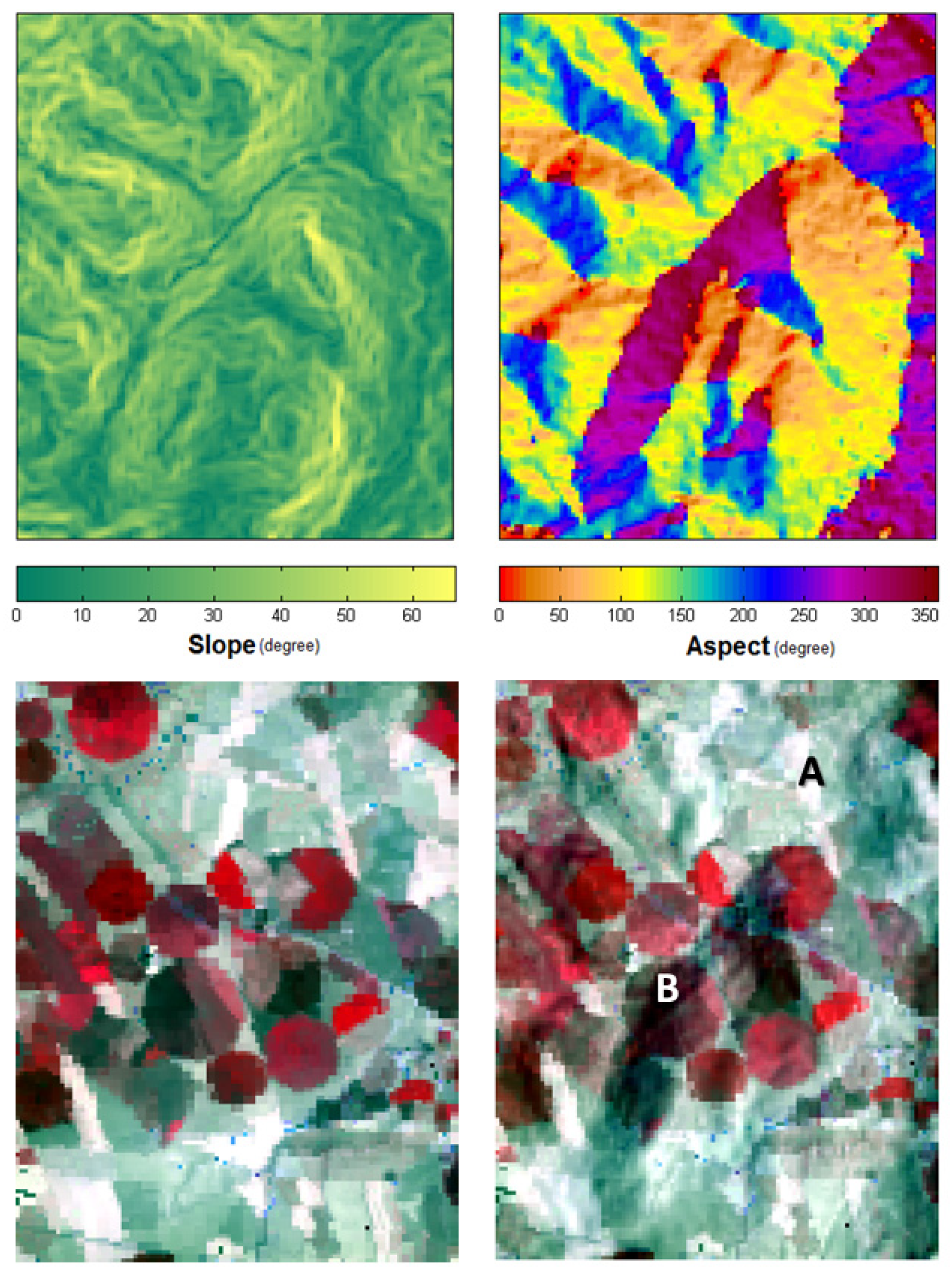
6.1. Topography Effects on the TOA Radiance


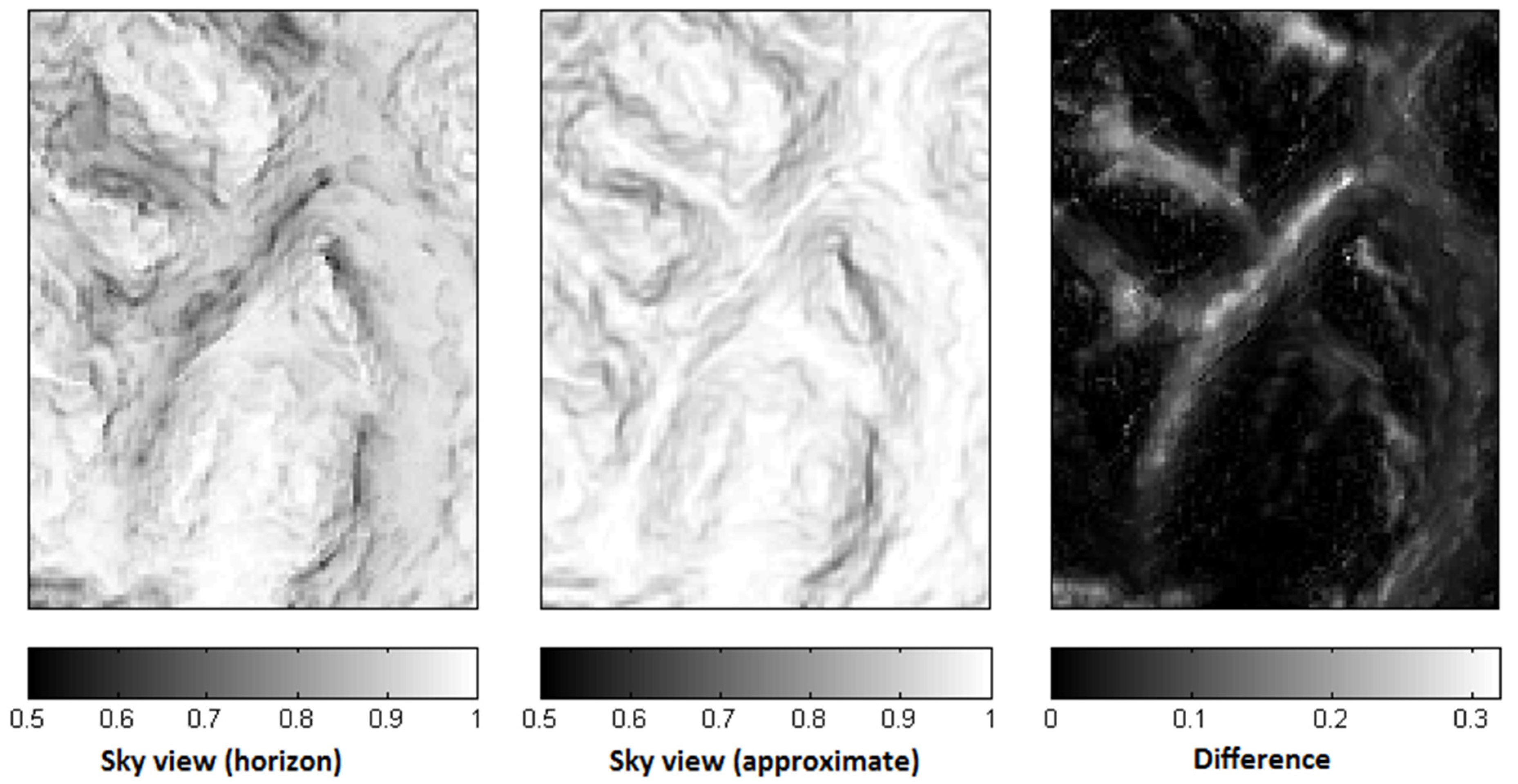
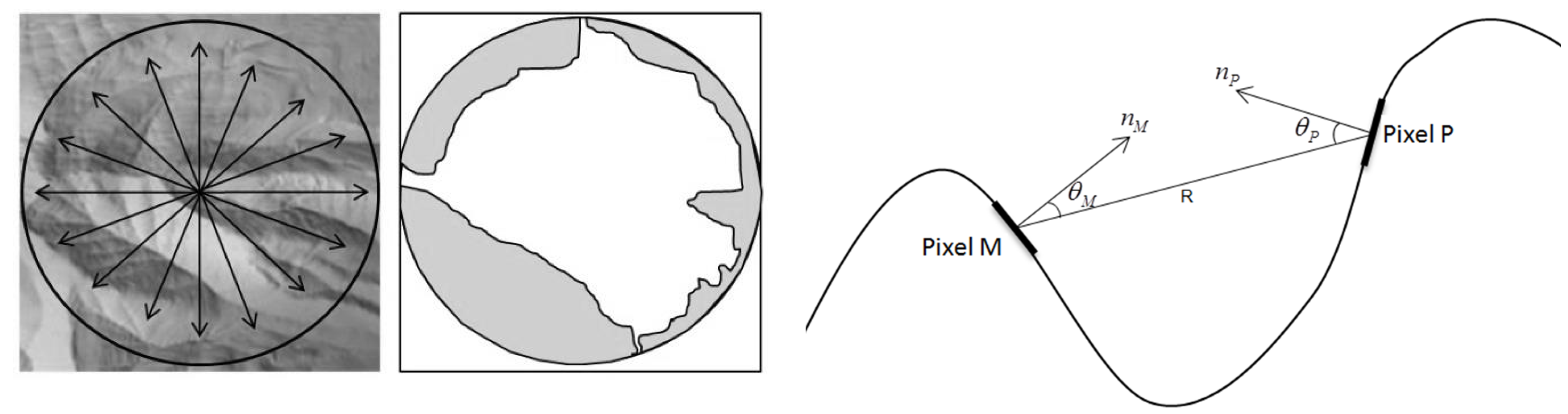
6.2. Sky View Factor Effect


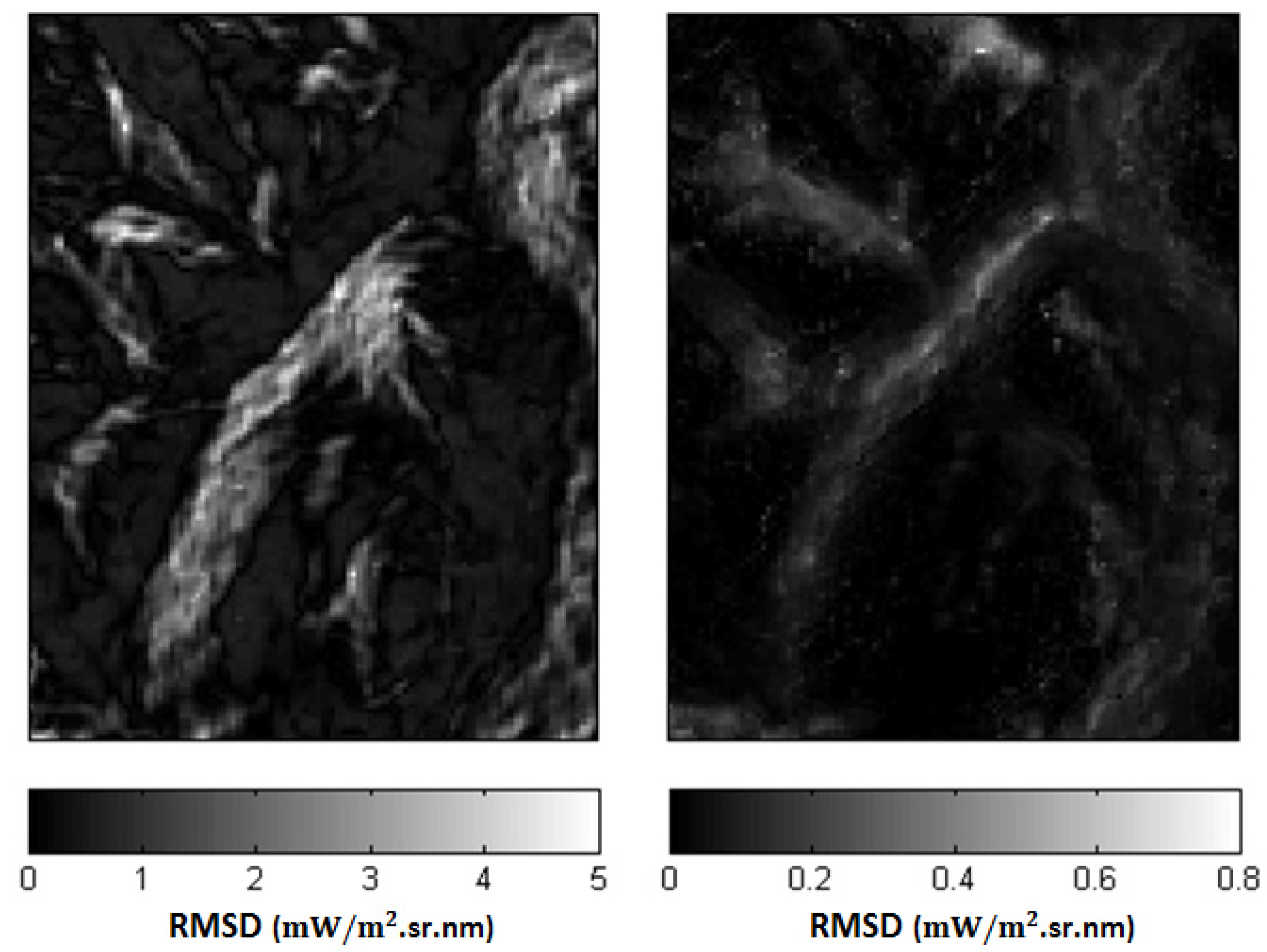
6.3. Terrain Reflected Radiance Effect
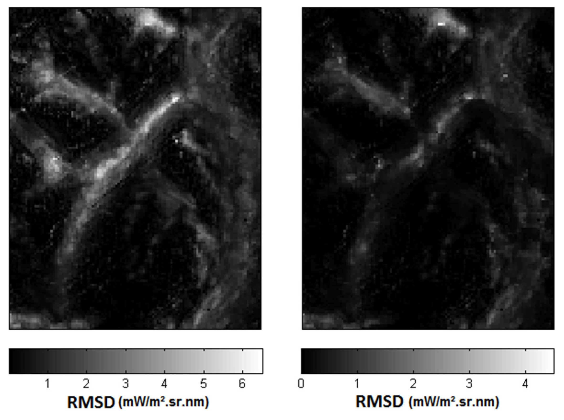

| Between Simulations with | RMSD (mW/m2·sr·nm) |
|---|---|
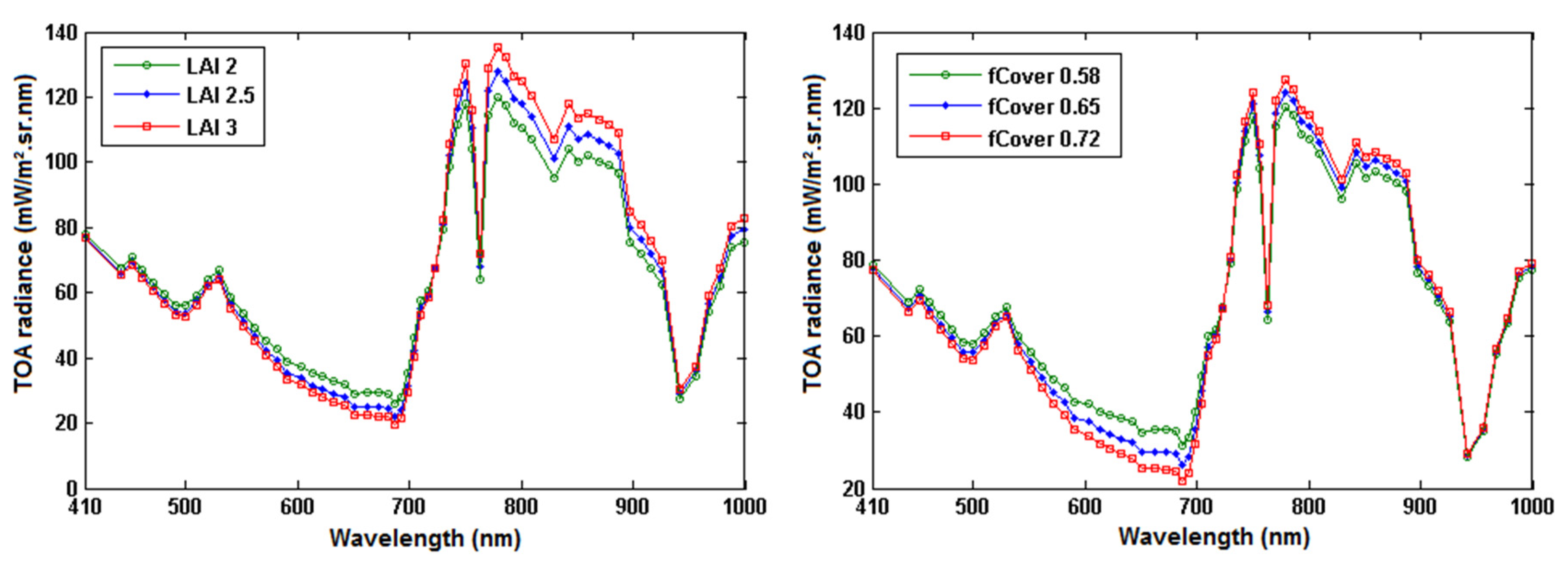
| LAI of 2 and LAI of 2.5 | 4.4 |
| LAI of 2.5 and LAI of 3 | 3.9 |
| LAI of 2 and LAI of 3 | 8.2 |
| fCover of 0.58 and fCover of 0.65 | 3.2 |
| fCover of 0.65 and fCover of 0.72 | 2.7 |
| fCover of 0.58 and fCover of 0.72 | 9 |
7. Conclusions
Acknowledgements
Author Contributions
Conflicts of Interest
References
- Laurent, V.C.E.; Verhoef, W.; Clevers, J.G.P.W.; Schaepman, M.E. Estimating forest variables from top-of-atmosphere radiance satellite measurements using coupled radiative transfer models. Remote Sens. Environ. 2011, 115, 1043–1052. [Google Scholar]
- Bacour, C.; Baret, B.; Béal, D.; Weiss, M.; Pavageau, K. Neural network estimation of LAI, fAPAR, fCover and LAI×Cab, from top of canopy MERIS reflectance data: Principles and validation. Remote Sens. Environ. 2006, 105, 313–325. [Google Scholar] [CrossRef]
- Baret, F.; Hagolle, O.; Geiger, B.; Bicheron, P.; Miras, B.; Huc, M.; Berthelot, B.; Niño, F.; Weiss, M.; Samain, O.; et al. LAI, fAPAR and fCover CYCLOPES global products derived from VEGETATION Part 1: Principles of the algorithm. Remote Sens. Environ. 2007, 110, 275–286. [Google Scholar] [CrossRef]
- Combal, B.; Baret, F.; Weiss, M.; Trubuil, A.; Macé, D.; Pragnère, A.; Myneni, R.; Knyazikhin, Y.; Wang, L. Retrieval of canopy biophysical variables from bidirectional reflectance: Using prior information to solve the ill-posed inverse problem. Remote Sens. Environ. 2002, 84, 1–15. [Google Scholar] [CrossRef]
- D’Urso, G.; Gomez, S.; Vuolo, F.; Dini, L. Estimation of land surface parameters through modeling inversion of earth observation optical data. In Advances in Modeling Agricultural Systems; Springer: New York, NY, USA, 2009; Volume 25, pp. 317–338. [Google Scholar]
- Goel, N.S. Models of vegetation canopy reflectance and their use in estimation of biophysical parameters from reflectance data. Remote Sens. Rev. 1988, 4, 1–212. [Google Scholar] [CrossRef]
- Goetz, A.F.H. Multi-Sensor analysis of NDVI, surface temperature and biophysical variables at a mixed grassland site. Int. J. Remote Sens. 1997, 18, 71–94. [Google Scholar] [CrossRef]
- Moreno, J.F.; Menenti, M.; Baret, F.; Rast, M.; Leroy, M.; Shaepman, M. Retrieval of vegetation properties from combined hyperspectral/multiangular optical measurements: Results from the DAISEX campaigns. In Proceedings of the IEEE International Geoscience and Remote Sensing Symposium, Toulouse, France, 21–25 July 2003.
- Schlerf, M.; Atzberger, C. Inversion of a forest reflectance model to estimate structural canopy variables from hyperspectral remote sensing data. Remote Sens. Environ. 2006, 100, 281–294. [Google Scholar] [CrossRef]
- Tang, S.; Chen, J.M.; Zhu, Q.; Li, X.; Chen, M.; Sun, R.; Zhou, Y.; Deng, F.; Xie, D. LAI inversion algorithm based on directional reflectance kernels. J. Environ. Manag. 2007, 85, 638–648. [Google Scholar] [CrossRef] [PubMed]
- Laurent, V.C.E.; Verhoef, W.; Clevers, J.G.P.W.; Schaepman, M.E. Inversion of a coupled canopy–atmosphere model using multi-angular top-of-atmosphere radiance data: A forest case study. Remote Sens. Environ. 2011, 115, 2603–2612. [Google Scholar] [CrossRef]
- Mousivand, A.; Menenti, M.; Gorte, B.; Verhoef, W. Global sensitivity analysis of the spectral radiance of a soil–vegetation system. Remote Sens. Environ. 2014, 145, 131–144. [Google Scholar] [CrossRef]
- Verhoef, W.; Bach, H. Coupled soil-leaf-canopy and atmosphere radiative transfer modeling to simulate hyperspectral multi-angular surface reflectance and TOA radiance data. Remote Sens. Environ. 2007, 109, 166–182. [Google Scholar] [CrossRef]
- Mousivand, A.; Menenti, M.; Gorte, B.; Verhoef, W. Multi-Temporal, multi-sensor retrieval of terrestrial vegetation properties from spectral–directional radiometric data. Remote Sens. Environ. 2015, 158, 311–330. [Google Scholar] [CrossRef]
- Bacour, C.; Jacquemoud, S.; Tourbier, Y.; Dechambre, M.; Frangi, J.P. Design and analysis of numerical experiments to compare four canopy reflectance models. Remote Sens. Environ. 2002, 79, 72–83. [Google Scholar] [CrossRef]
- Jacquemoud, S.; Verhoef, W.; Baret, F.; Bacour, C.; Zarco-Tejada, P.J.; Asner, G.P.; François, C.; Ustin, S.L. PROSPECT+SAIL models: A review of use for vegetation characterization. Remote Sens. Environ. 2009, 113, S56–S66. [Google Scholar] [CrossRef]
- Verhoef, W.; Bach, H. Remote sensing data assimilation using coupled radiative transfer models. Phys. Chem. Earth 2003, 28, 3–13. [Google Scholar] [CrossRef]
- Börner, A.; Wiest, L.; Keller, P.; Reulke, R.; Richter, R.; Schaepman, M.; Schläpfer, D. SENSOR: A tool for the simulation of hyperspectral remote sensing systems. ISPRS J. Photogramm. Remote Sens. 2001, 55, 299–312. [Google Scholar] [CrossRef]
- Fourty, T.; Baret, F. Vegetation water and dry matter contents estimated from top-of-the-atmosphere reflectance data: A simulation study. Remote Sens. Environ. 1997, 61, 34–45. [Google Scholar]
- Guanter, L.; Segl, K.; Kaufmann, H. Simulation of optical remote-sensing scenes with application to the EnMAP hyperspectral mission. IEEE Trans. Geosci. Remote Sens. 2009, 47, 2340–2351. [Google Scholar] [CrossRef]
- Isaacs, R.G.; Vogelmann, A.M. Multispectral sensor data simulation modeling based on the multiple scattering LOWTRAN code. Remote Sens. Environ. 1988, 26, 75–99. [Google Scholar] [CrossRef]
- Kerekes, J.P.; Landgrebe, D.A. Simulation of optical remote sensing systems. IEEE Trans. Geosci. Remote Sens. 1989, 27, 762–771. [Google Scholar] [CrossRef]
- Parente, M.; Clark, J.T.; Brown, A.J.; Bishop, J.L. End-to-end simulation and analytical model of remote-sensing systems: Application to CRISM. IEEE Trans. Geosci. Remote Sens. 2010, 48, 3877–3888. [Google Scholar] [CrossRef]
- Rahman, H.; Verstraete, M.M.; Pinty, B. Coupled surface-atmosphere reflectance (CSAR) Model 1. Model description and inversion on synthetic data. J. Geophys. Res. 1993, 98, 20779–20789. [Google Scholar] [CrossRef]
- Schott, J.R.; D. Brown, S.; V. Raqueno, R.; N. Gross, H.; Robinson, G. In advanced synthetic image generation models and their application to multi/hyperspectral algorithm development. In Proceedings of the 27th AIPR Workshop: Advances in Computer-Assisted Recognition, Washington, DC, USA, 14 October 1998.
- Verhoef, W.; Bach, H. Simulation of hyperspectral and directional radiance images using coupled biophysical and atmospheric radiative transfer models. Remote Sens. Environ. 2003, 87, 23–41. [Google Scholar] [CrossRef]
- Verhoef, W.; Bach, H. Simulation of Sentinel-3 images by four-stream surface–atmosphere radiative transfer modeling in the optical and thermal domains. Remote Sens. Environ. 2012, 120, 197–207. [Google Scholar] [CrossRef]
- Zhang, J.; Zhang, X.; Zou, B.; Chen, D. On hyperspectral image simulation of a complex woodland area. IEEE Trans. Geosci. Remote Sens. 2010, 48, 3889–3902. [Google Scholar] [CrossRef]
- Widlowski, J.L.; Taberner, M.; Pinty, B.; Bruniquel-Pinel, V.; Disney, M.; Fernandes, R.; Gastellu-Etchegorry, J.P.; Gobron, N.; Kuusk, A.; Lavergne, T.; et al. Third Radiation Transfer Model Intercomparison (RAMI) exercise: Documenting progress in canopy reflectance models. J. Geophys. Res. 2007, 112, D09111. [Google Scholar] [CrossRef]
- Laurent, V.C.E.; Verhoef, W.; Damm, A.; Schaepman, M.E.; Clevers, J.G.P.W. A Bayesian object-based approach for estimating vegetation biophysical and biochemical variables from APEX at-sensor radiance data. Remote Sens. Environ. 2013, 139, 6–17. [Google Scholar] [CrossRef]
- Gratton, D.J.; Howarth, P.J.; Marceau, D.J. Using Landsat-5 thematic mapper and digital elevation data to determine the net radiation field of a Mountain Glacier. Remote Sens. Environ. 1993, 43, 315–331. [Google Scholar] [CrossRef]
- Sanpedro, M.d.C.G. Optical and Radar Remote Sensing Applied to Agricultural Areas in Europe. Ph.D. Thesis, Délivré par l'Université Toulouse III, Toulouse, France, December 2008. [Google Scholar]
- Guanter, L.; Richter, R.; Kaufmann, H. On the application of the MODTRAN4 atmospheric radiative transfer code to optical remote sensing. Int. J. Remote Sens. 2009, 30, 1407–1424. [Google Scholar] [CrossRef]
- Vermote, E.F.; Tanre, D.; Deuz´e, J.L.; Herman, M.; Morcrette, J.J. Second simulation of the satellite signal in the solar spectrum, 6S: An overview. IEEE Trans. Geosci. Remote Sens. 1997, 35, 675–686. [Google Scholar] [CrossRef]
- Schott, J.R. Remote Sensing: The Image Chain Approach; Oxford University Press: Oxford, UK, 2007. [Google Scholar]
- Sandmeier, S.; Itten, K.I. A physically-based model to correct atmospheric and illumination effects in optical satellite data of rugged terrain. IEEE Trans. Geosci. Remote Sens. 1997, 35, 708–717. [Google Scholar] [CrossRef]
- Dozier, J.; Bruno, J.; Downey, P. A faster solution to the horizon problem. Comput. Geosci. 1981, 7, 145–151. [Google Scholar] [CrossRef]
- Proy, C.; Tanré, D.; Deschamps, P.Y. Evaluation of topographic effects in remotely sensed data. Remote Sens. Environ. 1989, 30, 21–32. [Google Scholar] [CrossRef]
- Hay, J.E. Calculating solar radiation for inclined surfaces: Practical approaches. Renew. Energy 1993, 3, 373–380. [Google Scholar] [CrossRef]
- Liu, B.Y.H.; Jordan, R.C. The interrelationship and characteristic distribution of direct, diffuse and total solar radiation. Solar Energy 1960, 4, 1–19. [Google Scholar] [CrossRef]
- Rakovec, J.; Zakšek, K. On the proper analytical expression for the sky-view factor and the diffuse irradiation of a slope for an isotropic sky. Renew. Energy 2012, 37, 440–444. [Google Scholar] [CrossRef]
- Dozier, J.; Frew, J. Rapid calculation of terrain parameters for radiation modeling from digital elevation data. IEEE Trans. Geosci. Remote Sens. 1990, 28, 963–969. [Google Scholar] [CrossRef]
- Richter, R. Correction of satellite imagery over mountainous terrain. Appl. Opt. 1998, 37, 4004–4015. [Google Scholar] [CrossRef] [PubMed]
- Richter, R.; Schläpfer, D. Geo-Atmospheric processing of airborne imaging spectrometry data Part 2: Atmospheric/topographic correction. Int. J. Remote Sens. 2002, 23, 2631–2649. [Google Scholar] [CrossRef]
- Berk, A.; Anderson, G.P.; Acharya, P.K.; Hoke, M.L.; Chetwynd, J.H.; Bernstein, L.S.; Shettle, E.P.; Matthew, M.W.; Adler-Golden, S.M. MODTRAN4 Version 3 Revision 1 User’s Manual; Technical Report; Air Force Research Laboratory: Hanscom Air Force Base, MA, USA, 2003. [Google Scholar]
- Berk, A.; Bernstein, L.S.; Anderson, G.P.; Acharya, P.K.; Robertson, D.C.; Chetwynd, J.H.; Adler-Golden, S.M. MODTRAN cloud and multiple scattering upgrades with application to AVIRIS. Remote Sens. Environ. 1998, 65, 367–375. [Google Scholar] [CrossRef]
- Schläpfer, D.; Nieke, J. Operational simulation of at sensor radiance sensitivity using the MODO/MODTRAN4 environment. In Proceedings of the 4th EARSeL Workshop on Imaging Spectroscopy. New Quality in Environmental Studies, Warsaw, Poland, 27–30 April 2005.
- Adler, S.M.; Matthew, M.W.; Bernstein, L.S.; Levine, R.Y.; Berk, A.; Richtsmeier, S.C.; Acharya, P.K.; Anderson, G.P.; Felde, G.; Gardner, J.; et al. Atmospheric correction for short-wave spectral imagery based on MODTRAN4. Proc. SPIE 1999, 3753, 61–69. [Google Scholar]
- Brockmann, C.; Kirches, G.; Kirches, S.; Geißler, J.; Krämer, U.; Faber, E.; Soria, G.; Mattar, C.; Jimenez, J.C.; Franch, B.; et al. Sentinel-3 Experimental Campaign (SEN3EXP) Final Report; ESA Contract No. 22661/09/I-LG; ESA Publications Division: Noordwijk, The Netherlands, 2011. [Google Scholar]
- Richter, R. Correction of atmospheric and topographic effects for high spatial resolution satellite imagery. Int. J. Remote Sens. 1997, 18, 1099–1111. [Google Scholar] [CrossRef]
- Martimort, P.; Berger, M.; Carnicero, B.; Bello, U.D.; Fernandez, V.; Gascon, F.; Silvestrin, P.; Spoto, F.; Sy, O. Sentinel-2 – the optical high-resolution mission for GMES operational services. ESA Bull. 2007, 131, 18–23. [Google Scholar]
© 2015 by the authors; licensee MDPI, Basel, Switzerland. This article is an open access article distributed under the terms and conditions of the Creative Commons Attribution license (http://creativecommons.org/licenses/by/4.0/).
Share and Cite
Mousivand, A.; Verhoef, W.; Menenti, M.; Gorte, B. Modeling Top of Atmosphere Radiance over Heterogeneous Non-Lambertian Rugged Terrain. Remote Sens. 2015, 7, 8019-8044. https://doi.org/10.3390/rs70608019
Mousivand A, Verhoef W, Menenti M, Gorte B. Modeling Top of Atmosphere Radiance over Heterogeneous Non-Lambertian Rugged Terrain. Remote Sensing. 2015; 7(6):8019-8044. https://doi.org/10.3390/rs70608019
Chicago/Turabian StyleMousivand, Alijafar, Wout Verhoef, Massimo Menenti, and Ben Gorte. 2015. "Modeling Top of Atmosphere Radiance over Heterogeneous Non-Lambertian Rugged Terrain" Remote Sensing 7, no. 6: 8019-8044. https://doi.org/10.3390/rs70608019
APA StyleMousivand, A., Verhoef, W., Menenti, M., & Gorte, B. (2015). Modeling Top of Atmosphere Radiance over Heterogeneous Non-Lambertian Rugged Terrain. Remote Sensing, 7(6), 8019-8044. https://doi.org/10.3390/rs70608019