Sensitivity of a Floodplain Hydrodynamic Model to Satellite-Based DEM Scale and Accuracy: Case Study—The Atchafalaya Basin

Abstract

The hydrodynamics of low-lying riverine floodplains and wetlands play a critical role in hydrology and ecosystem processes. Because small topographic features affect floodplain storage and flow velocity, a hydrodynamic model setup of these regions imposes more stringent requirements on the input Digital Elevation Model (DEM) compared to upland regions with comparatively high slopes. This current study provides a systematic approach to evaluate the required relative vertical accuracy and spatial resolution of current and future satellite-based altimeters within the context of DEM requirements for 2-D floodplain hydrodynamic models. A case study is presented for the Atchafalaya Basin with a model domain of 1190 km². The approach analyzes the sensitivity of modeled floodplain water elevation and velocity to typical satellite-based DEM grid-box scale and vertical error, using a previously calibrated version of the physically-based flood inundation model (LISFLOOD-ACC). Results indicate a trade-off relationship between DEM relative vertical error and grid-box size. Higher resolution models are the most sensitive to vertical accuracy, but the impact diminishes at coarser resolutions because of spatial averaging. The results provide guidance to engineers and scientists when defining the observation scales of future altimetry missions such as the Surface Water and Ocean Topography (SWOT) mission from the perspective of numerical modeling requirements for large floodplains of O[10³] km² and greater.

1. Introduction

Floodplains and associated wetlands play critical roles in climate by their impact on hydrologic and biogeochemical processes [1]. Over the past 200 years, the loss of wetlands in the United States has been estimated to be approximately 50%, with similar or greater loss rates in parts of Europe, Australia, Canada, and Asia [2].

Effective computer modeling and monitoring of floodplain dynamics are essential for understanding methane production, sediment transport, and nutrient exchanges [3]. Modeled flood forecasts and delineation of flood prone areas are especially sensitive to the representation of topography [4,5,6,7]. With continued advances in the development of river discharge algorithms from remote sensing [8,9,10] and the increasing availability of space-based global Digital Elevation Models (DEMs), such as the Shuttle Radar Topography Mission (SRTM) [11] and the Advanced Spaceborne Thermal Emission and Reflection Radiometer (ASTER) Global Digital Elevation Model (GDEM) [12], the merging of hydraulic and remote-sensing analyses is becoming increasingly important. Given the nonlinear dynamics of floodplain flows, a reasonable approach to investigate this problem is running numerical models at various DEM scales and accuracies to compare modeled errors.

Various shallow-water-flow models have proven to be useful tools when computing in- and over-bank fluvial hydraulics in scientific and engineering research [4]. They range from empirical routing to more-sophisticated numerical solutions to the full St. Venant equations. The simpler 1-D versions are computationally efficient, typically requiring a series of cross sections of channel and floodplain topography derived from ground surveys. Such models have often provided good predictions of bulk flow and flood extent despite limited topographic and cross-sectional data [13].

Despite their extensive use for channel flow, 1-D models cannot replicate the lateral movement of the flood wave in what is a highly two-dimensional (2-D) process [14]. The 1-D models often overestimate the floodplain extension because they do not include the volume information in the floodplain delineation. Consequently, 2-D models have gained credence in modeling of the extent of floodplain-flow inundation [15,16]. These models typically use a 1-D representation of channel flow linked to a 2-D treatment of flow over the floodplain, discretized into a grid of square cells or irregular polygonal units, e.g., [17,18]. Studies indicate that 2-D floodplain-flow models also have been constrained by the scarcity of high-resolution topographic data [19,20], although airborne surveys and a basic process representation provide good predictions of flood inundation extent at the local scale [21]. Knowledge of rule curves for river diversions or other floodplain-control structures are required for representative floodplain simulations.

Precise DEMs are therefore required for the accurate modeling of floodplain hydrodynamics, commensurate with the 2-D model. High-resolution satellite-based altimetry is an obvious source, especially for large regions and global coverage. Both space-based and airborne DEMs are used for 2-D floodplain hydrodynamic models targeting small basins, e.g., [15,22] and for evaluating floodplain-elevation profiles in continental-scale river models, e.g., [23,24]. Early inundation modeling studies have become possible because airborne Light Detection And Ranging (LiDAR) provide high spatial resolution (1 m) topography with high vertical accuracy (±15 cm), e.g., [19,25,26].

Although a viable alternative, the accuracy of currently available space-based DEMs is hindered by a variety of errors (e.g., missing vector features such as drainage ditches and embankment heights, pits caused by vegetation canopies, subpixel-sized structures, and random radar speckles), which, from the perspective of hydraulic modeling, reduce the flow connectivity between river channels and the surrounding floodplains [27,28]. Space-based DEMs, such as SRTM [11] and ASTER GDEM [12], have an advantage in covering almost the entire earth. The typical spatial resolutions of space-based DEMs (i.e., 90 m in SRTM and 30 m in ASTER GDEM) are not fine enough to represent such small structures as narrow channels connecting main rivers and floodplains [29]. These problems in space-based DEMs are often not present in LiDAR-based measurements, which have higher spatial resolution [30], although spatial coverage and repeat frequency are limited in single-track sensors. Future altimetry missions, however, such as the Surface Water and Ocean Topography (SWOT) mission [31], the Deformation, Ecosystem Structure, and Dynamics of Ice (DESDynI) mission [32], and the second-generation Ice, Cloud, and land-Elevation Satellite (ICESat-2) mission, should be capable of providing global DEMs with submeter accuracy in remote areas.

The sensitivity analyses of 2-D hydrodynamic models to DEMs have been limited mostly to investigating urban and peri-urban flood events with airborne LiDAR [21,33]. Urban environments are characterized by high spatial-height variability; thus urban models require detailed representation of buildings. Two-dimensional hydrodynamic modeling studies have focused on rural flooding on flat alluvial plains [27] with few small-scale artificial features, and thus have been run at coarser resolution DEM, e.g., [29].

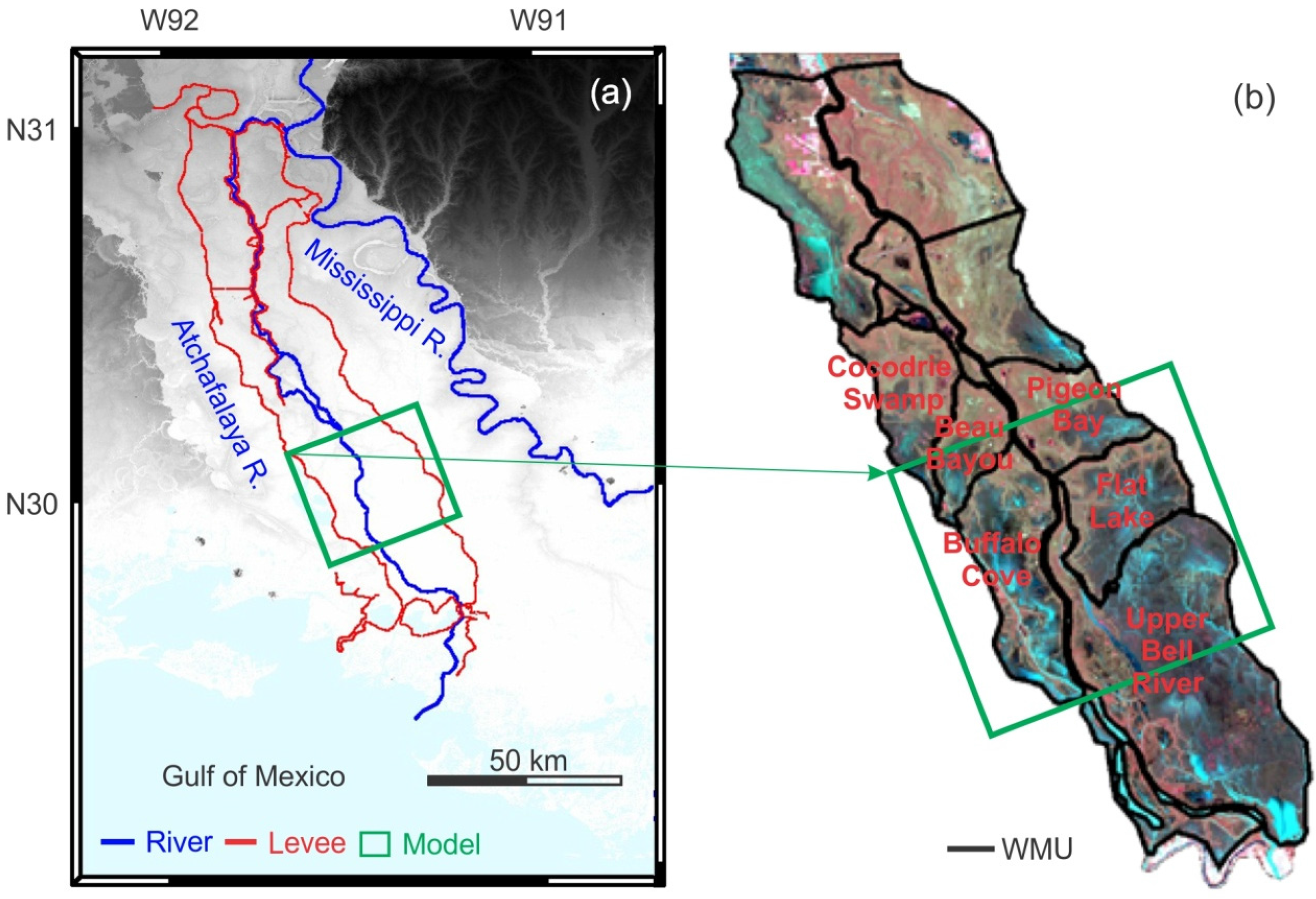
The focus of this paper is to analyze 2-D floodplain model sensitivity to grid-box size associated with current and anticipated upcoming space-based altimetry, using a previously calibrated model on the Atchafalaya floodplain [34]. The goal is to evaluate the trade-off between DEM spatial resolution and relative vertical accuracy for larger floodplains (O[10³] km² and greater) that can employ current and near-future altimeter data. The relative vertical accuracy, accounts for random errors, as compared to the absolute accuracy that also includes the effect of systematic error. For floodplain modeling, the relative vertical accuracy of the DEM is appropriate as it focuses on local differences among adjacent elevation values, such as slope and aspect.

This sensitivity is evaluated in terms of water elevation and velocity during overbank flooding. During low flows, the intricacies of channel geometry are of significance to the floodplain hydrodynamics [35], whereas at high flows, the whole floodplain and valley floor begin to behave as a single-channel unit. To address the full range of spring-flood filling and subsequent flow-recession, a two-month period from April to June, 2008, is chosen.

This result is thus a systematic assessment of satellite-based DEM needs for riverine floodplain model, and the capability of satellites to meet those needs. The goal is to not only understand the sensitivity of hydrodynamic models to both vertical DEM error and grid-box resolution, but also to develop the trade-off between DEM vertical error and grid-box size.

2. Methods

2.1. Study Area

The Atchafalaya River Basin is situated west of the Lower Mississippi River in south Louisiana within the coastal margin of the Gulf of Mexico. This drainage basin with an area of 5670 km² includes bottomland hardwoods, swamps, bayous, and backwater lakes [36,37] in the United States, holding a rich abundance and diversity of terrestrial and aquatic species. The Atchafalaya River’s immense floodplain is bounded by levees on the east and west sides separated by 20 to 30 km. Prior to reaching the Gulf of Mexico, the Atchafalaya River is modified by a network of natural and artificial water diversions and is constrained by flood and navigation control structures [38]. Gates along the main stem divert nearly 30% of Mississippi River water into the Atchafalaya River, and this flows south through the floodplain to the Gulf of Mexico along a reach of approximately 225 km [39].

Figure 1 shows the location map including rivers, levees, and model area. It includes six out of thirteen U.S. Army Corps of Engineers (USACE) subbasins or Water Management Units (WMUs) within the basin, identified based on morphological diversity [40]. The six WMUs are selected for this study primarily because their upstream, downstream, and lateral boundaries are well defined, and high-resolution airborne DEMs are available. WMUs Cocodrie Swamp and Beau Bayou on the right bank and Pigeon Bay on the left bank represent the upper domain boundaries with a time-dependent floodplain discharge. WMU’s Buffalo Cove on the right bank and Flat Lake and Upper Bell River on the left bank are the main model areas to evaluate how overbank flooding disperses into the floodplain (see Figure 1b). All these WMUs are characterized by a swamp forest with paths of slowly moving water or bayous. The channel flow from upstream to downstream results in more overbank flooding into the floodplain.

Figure 1. (a) LiDAR map over the study area. The Atchafalaya Basin is bounded on the east and west sides by levees in southern Louisiana. The Atchafalaya River and the Mississippi River are represented by blue lines. Levees are marked with red lines. The green rectangular box represents the model study area. (b) The Landsat ETM+ color composite image represents water management units (WMU) outlined by black lines, courtesy of [37].

Figure 1. (a) LiDAR map over the study area. The Atchafalaya Basin is bounded on the east and west sides by levees in southern Louisiana. The Atchafalaya River and the Mississippi River are represented by blue lines. Levees are marked with red lines. The green rectangular box represents the model study area. (b) The Landsat ETM+ color composite image represents water management units (WMU) outlined by black lines, courtesy of [37].

2.2. Floodplain Hydrodynamic Model

The LISFLOOD-INT hydrodynamic model [41] was applied to this riverine floodplain. The base model uses a 1-D representation of channel flow coupled to a 2-D raster model for floodplain flow. Channel flow employs the diffusive approximation to the full 1-D St. Venant equations solved by using a fully implicit Newton-Raphson scheme. The 1-D channel model is vectorized along the main channel with input parameters of bathymetric depths, channel widths, and time-varying-flow boundary conditions.

Floodplain flows decoupled in x and y directions are implemented for a raster grid to give an approximation to a 2-D inertial wave. Mass conservation is simulated through the continuity equation (Equation (1)). The LISFLOOD-INT momentum equation includes local acceleration terms as a result of gravity, and it is solved using an explicit finite difference scheme (Equation (2)),

$$h_{i,j}^{t+\text{Δ}t}=h_{i,j}^t+\text{Δ}t\frac{Q_{xi,j-1}^t-Q_{xi,j}^t+Q_{yi,j-1}^t-Q_{yi,j}^t}{\text{Δ}{x}^2}$$

(1)

$$Q^t=\frac{q^t-g{h}_{flow}^t\text{Δ}t\frac{\text{Δ}\left(h^t+z\right)}{\text{Δ}x}}{\left(1+g{h}_{flow}^t\text{Δ}t{n}^2\left|q^{t-\text{Δ}t}\right|/{\left(h_{flow}^t\right)}^{10/3}\right)}\text{Δ}x$$

(2)

where $h$ is the cell water depth, $h_{flow}$ is the depth between cells through which water can flow, $Q$ is the flow between cells, $\text{Δ}x$ is the cell size, $\text{Δ}t$ is the time step, $n$ is Manning’s roughness coefficient, $q$ is $Q$ from the previous time step divided by cell width, and $g$ is gravity. This code allows quicker run times than previous LISFLOOD-FP variants [15], as well as better representation of the flow physics [41,42].

Overbank flow is the major contributor to the Atchafalaya floodplain inundation for the model period. As lateral inflow from channel to floodplain, this overbank flow is controlled by exchanges between the 1D channel and 2D raster models. When rising water elevation within the channel attains floodplain elevation around the channel, overbank flow begins to spill toward the floodplain.

The previously calibrated LISFLOOD-INT configuration described in [34] is implemented for this study. The study period was for 62 days, from April 1 to June 1, 2008, encompassing a spring high flood followed by a recession period. During the model period, the highest flood level occurred on 28 April 2008, whereas the lowest was June 1. The study area was surrounded by levees on both the east and west sides that are used for lateral boundary conditions (Figure 1). The man-made levees in the domain are narrow, typically less than 10 m wide, and sufficiently high, ~20 m, so that floodwaters reaching up to ~6 m in elevation cannot overtop them for the chosen simulation period. The USACE developed updated flood control, navigation maps, and hydrographic survey maps for the Atchafalaya River as part of a comprehensive mapping project [43]. The mapping project provided bathymetric depth measurements every 10 feet along the river cross sections. Based on the bathymetry data set, the average bed elevations and channel widths were calculated as equivalent area rectangular cross sections at about every 1 km along the 34 km reach of the main channel. Inflow boundary condition is set with time-dependent discharge at the upstream, and outflow boundary condition is set with the time-varying water elevation at the downstream based on local USGS gauge stations. No additional diversions by gates or other control structures within the study area are assumed. Topography is assumed static for each model run for the entire 62-day period. Constant Manning roughness coefficients of 0.028 for the channel ($n_C$) and 0.1 for the floodplain ($n_f$) were previously estimated from the calibration of LISFLOOD-INT for the same period using time series interferometry synthetic aperture radar [34].

The DEM averaging introduces several potential impacts. First, it can result in a terrain data error as a result of smoothing out topography relevant to the flow hydraulics, such as levees on the east and west boundaries of the model domain. Further, the presence of significant structural features, including, levees, houses, walls, and others, on a river floodplain is important in relation to both the volume of the floodplain that can be occupied by the flow and the direction it takes across the floodplain [21]. To handle these subgrid-scale features [44], the levees in 1-m resolution were vectorized and extracted, and the mean levee elevation was directly input into the levee location at each DEM resolution. With increasing grid-box size, natural levees along the channel (hereinafter referred to as “floodplain bank” or “bank”) were smoothed along with floodplain. However, in order to constrain the flow within the Atchafalaya basin, levees at both the eastern and western boundaries of the modeling domain were set to the spatially uniform height so that no water was spilled into adjacent basins.

The sensitivity of grid-box size was tested using five scales, 50, 100, 250, 500, and 1000 m, each with three different vertical errors of 0, 0.5, and 1 m. The 50-m high-resolution control or “benchmark” floodplain elevation map was directly averaged to obtain the lower-resolution maps. The different vertical DEM errors were synthetically generated as described in Section 2.3 illustrated in Figure 2, and summarized in Table 1. Model sensitivity was carried out by evaluating the 15 different model configurations, which produced different water elevations and velocities with respect to the calibrated benchmark case. Error was quantified using the Root Mean Square Error (RMSE) as follows:

$$RMSE=\sqrt{{\displaystyle \sum }_{i=1}^N{(B_i-T_i)}^2/N}$$

(3)

where $T$ and $B$ are, respectively, the outputs of test models and the benchmark high-resolution model, $\overline{B}$ is the mean value of the benchmark model outputs, and N is the number of model outputs.

Figure 2. Space-based floodplain digital elevation (Z) maps synthetically generated for floodplain model-sensitivity analysis.

Figure 2. Space-based floodplain digital elevation (Z) maps synthetically generated for floodplain model-sensitivity analysis.

Table 1. RMSE of the synthetic floodplain elevation maps in Figure 2 with respect to 50 m benchmark and nonerror elevation map (Z_{∆50, σ0}).

Unit: m	Z∆50	Z∆100	Z∆250	Z∆500	Z∆1000
Zσ0		0	0	0	0
Zσ1	0.50	0.25	0.10	0.05	0.02
Zσ2	1.00	0.50	0.20	0.10	0.05

Table 1. RMSE of the synthetic floodplain elevation maps in Figure 2 with respect to 50 m benchmark and nonerror elevation map (Z_{∆50, σ0}).

Unit: m	Z∆50	Z∆100	Z∆250	Z∆500	Z∆1000
Zσ0		0	0	0	0
Zσ1	0.50	0.25	0.10	0.05	0.02
Zσ2	1.00	0.50	0.20	0.10	0.05

2.3. Generation of Synthetic Space-based Digital Elevation Maps

Space-based DEMs from imaging methods (e.g., radar interferometer and digital photogrammetry) provide meter-scale vertical accuracy. For example, SRTM, using a C-band (5.6-cm wavelength) Interferometric Synthetic Aperture Radar (InSAR), shows a relative height accuracy for North America of 7 m for 30-m pixel in 90% errors [30]. The ASTER GDEM, generated from a stereo-pair of images acquired with nadir and backward angles over the same area, yields an RMSE in vertical accuracy of approximately 9 m for 30-m pixel over the conterminous United States [45,46]. In contrast, despite being unable to provide 2-D maps, space-based DEMs from profiling methods (e.g., radar altimeter and LiDAR) provide submeter vertical accuracy, just as any airborne sensors will. For example, the Geoscience Laser Altimeter System (GLAS) aboard the Ice, Cloud and Land Elevation Satellite (ICESat) mission enabled the separation of vegetation canopy heights from the ground and provided a bare earth along-track elevation with an accuracy of about 15 cm [47] for approximately 65-m pixel scales. The SWOT and DESDynI missions previously proposed to combine two types of space-based sensors that taken together provide 2-D earth observations with vertical accuracy less than 1 m for 10-m spatial resolution [31,32].

The floodplain topography for the current study was constructed starting with a high-resolution 1 m LiDAR DEM of the whole basin published by USGS National Geospatial Program and USGS Coastal and Marine Geology Program [48]. The airborne LiDAR survey was acquired in November 2010 during an optimal data collection window in terms of average river stage, average minimum temperature, and tree canopy. The LiDAR vertical accuracy was 18.5 cm RMSE. The 1-m LiDAR DEM was aggregated to 50 m as the benchmark or true grid-box size, which is typical of satellite-based land-surface altimeters including SWOT [31]. Coarser resolution DEMs were generated by aggregating the 50-m DEM tolarger scales.

For the model sensitivity study, a zero-mean Gaussian random vertical error with standard deviation of 0.5 m (σ1) and 1 m (σ2) for a grid-box size of 50 m was generated, corresponding with the approximate typical relative vertical uncertainty estimate of the upcoming satellite altimetry missions. The error was added to the benchmark scale elevation maps associated with σ0 (no error) to create σ1 and σ2 maps. They were then averaged to four progressively coarser resolutions of 100, 250, 500, and 1000 m, respectively (Figure 2). These scales were determined based on the SWOT hydrologic science requirement. The SWOT mission will provide all terrestrial surface water bodies whose surface area (e.g., lakes, reservoirs, wetlands) exceeds 1 km² (goal, 250 m²) and rivers whose width exceeds 100 m (goal, 50 m) [31]. The random error is spatially uncorrelated and reduces linearly in proportion to $1/\sqrt{n}$ as the data are aggregated, where n is the number of pixels being averaged. Potential bias due to vegetation canopy effects on DEM is not included because this study area is covered by a homogeneous swamp forest. Systematic errors were not introduced into the synthetically generated DEMs. For instance, long wavelength and spatially non-stationary behaviors due to residual roll errors are typically on the order of thousands of kilometers [11,30] and, thus, would not impact our comparatively small model domain.

In Figure 2, floodplain elevation maps in finer grid-box size become noisier than the coarser grids resulting from the additional error. Additionally, Table 1 shows that the RMSEs decrease exponentially with spatial aggregation. The RMSEs in a 1000-m grid-box size drop to 2 cm for σ1 and to 5 cm for σ2.

3. Results

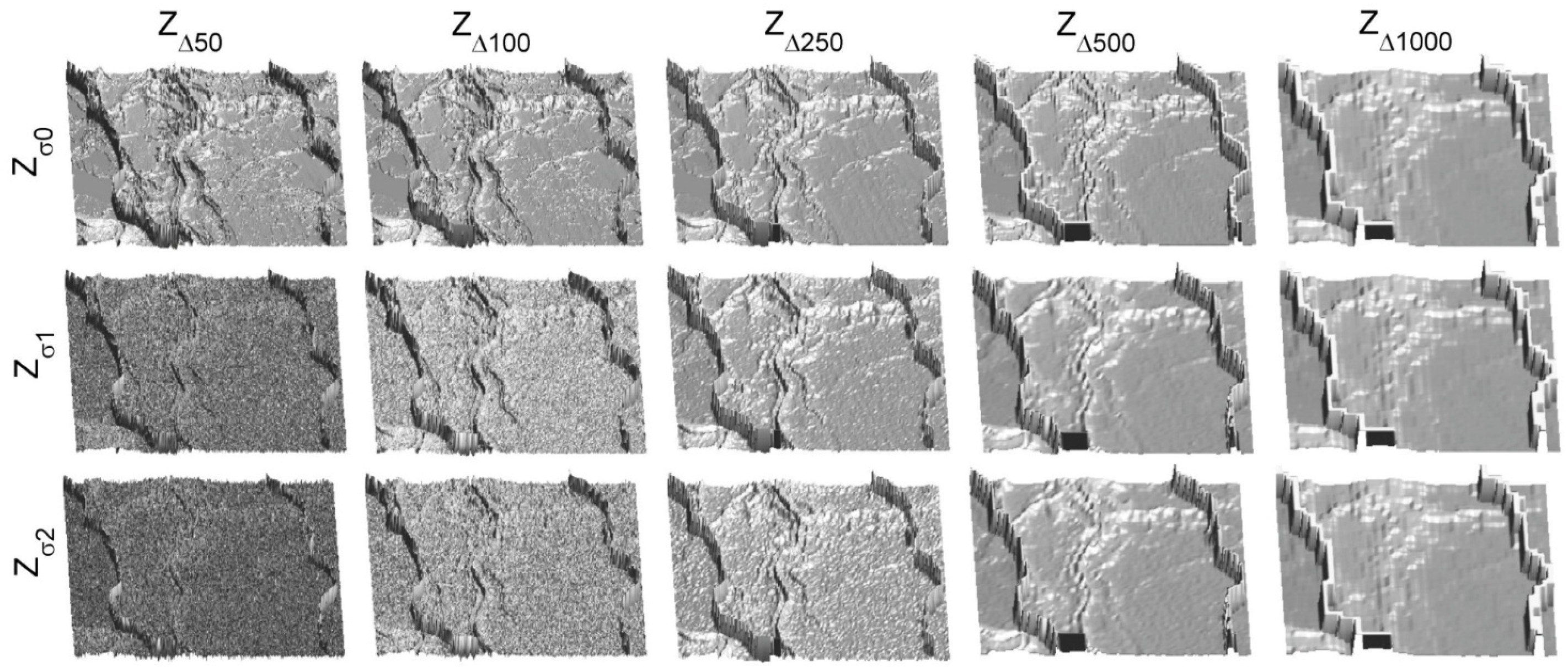
The different floodplain DEMs consisting of 50-, 100-, 250-, 500-, and 1000-m grid-box sizes, each with three DEM errors of σ0 (no error), σ1 (0.5 m/50 m), and σ2 (1 m/50 m) were used in generating 15 hydrodynamic modeling scenarios. Once simulated, the modeled elevations and flows were compared to the benchmark run using various statistics, as described below. Results were evaluated during both high- and low-water conditions.

3.1. Sensitivity of Model Water Elevation to Grid-Box Size and DEM Error

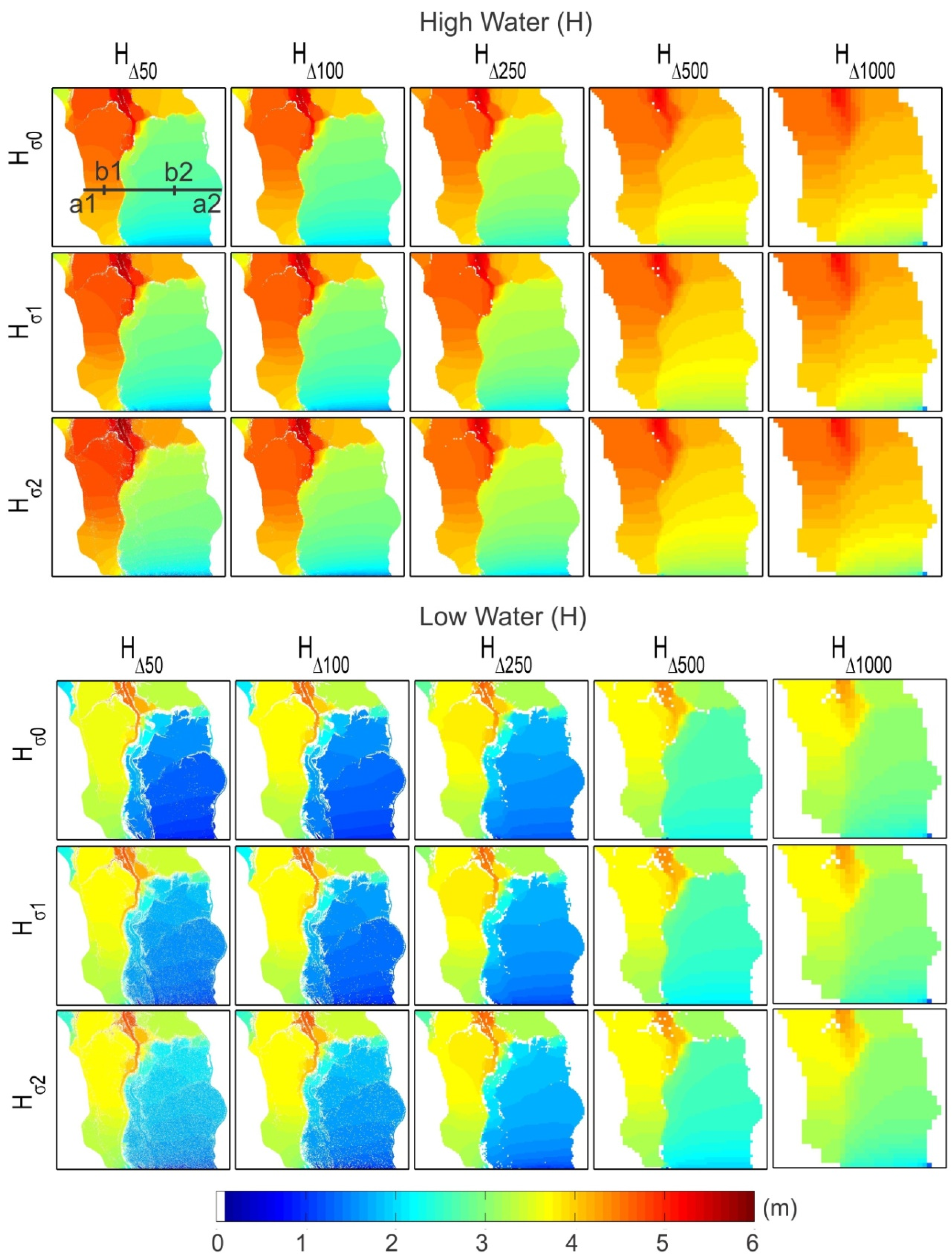
Water elevation maps during high- and low-water periods from the 15 different hydrodynamic cases are shown in Figure 3. Overall, the simulations indicate that overbank flow first enters the floodplain upstream on both the right and left banks. It then flows south, bounded by the floodplain banks. At high flows, water from the right bank then spills over to the left bank about midway through the study domain, contributing additional water to the larger left-bank floodplain. Water elevations of the high-water period are generally less than 2 m higher than those of low water in all cases.

Results indicate that both the coarsening of grid-box size and also DEM error have significant impacts on water elevation. First, coarsening alters the spatial water surface patterns of the subbasin WMUs by smoothing out topographic variability, including the subbasin boundaries at larger scales. For instance, WMU boundaries between Cocodrie Swamp and Beau Bayou on the right bank and between Pigeon Bay and Flat Lake on the left bank are clearly distinguished in the models of grid-box sizes 50, 100, and 250 m. But the same WMU boundaries are not apparent at 500- and 1000-m grid-box sizes. This is not surprising because resampling to larger scales increasingly fills the depressions and cuts off the peaks of the higher-resolution models.

Second, close inspection of Figure 3 seems to indicate that for both high- and low-water periods a much greater amount of spatial detail is lost in the water-surface elevation maps above 250 m compared to the higher-resolution cases, suggesting that the water surface is reasonably well represented up to a 250-m model. For instance, some high uplifted regions are not flooded (i.e., dry) at low water at finer resolutions. However, the elevations of these areas are lowered at with increasing aggregation and, thus, turn out to be flooded (i.e., wet). This result indicates that the model cannot reproduce spatial variations in hydraulics at a scale coarser than the element size or more than the mean-river width, estimated to be 356 m for the Atchafalaya study area. For model resolutions above this critical length threshold of mean river width, model performance deteriorates significantly, although it is also very likely to be dependent on water flow and geomorphology.

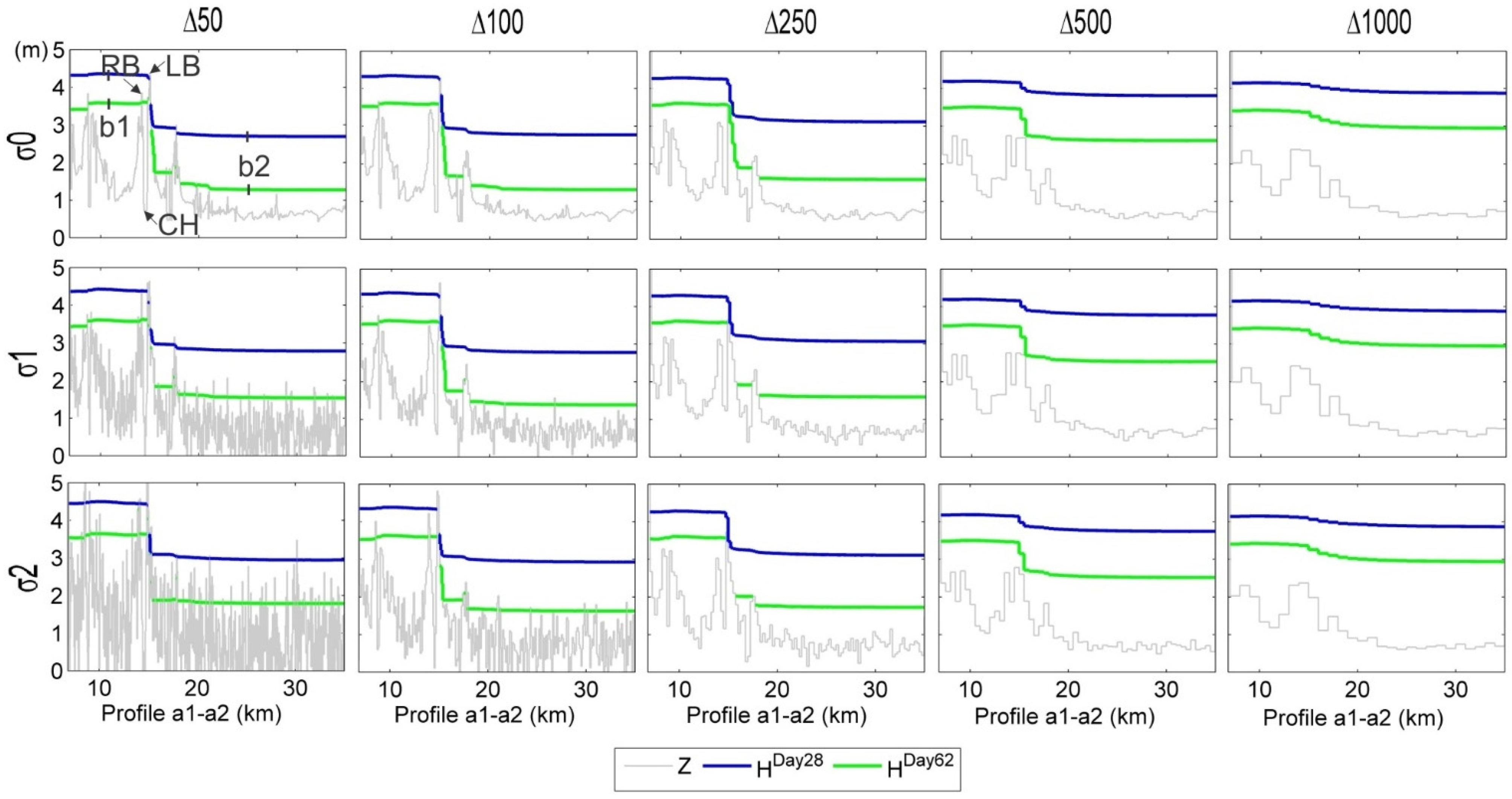
Third, resampling results in several significantly different impacts on the left- and right-bank floodplains. To compare those differences, a water elevation profile of the transect a1-a2 identified in Figure 3, is plotted for each case in Figure 4 for the high- and low-water periods. Overall, water elevations on the right bank are higher than those on the left bank as a result of the high floodplain banks at ~15 km on profile a1-a2. Moreover, as grid-box size increases, water elevations on the right bank slightly decrease while water elevations on the left bank increase to nearly approach the levels on the right bank. This result is a direct consequence of the smoothing effect at greater aggregations, which effectively reduces the modeled heights of the floodplain banks reducing their ability to contain the right-bank flow.

Figure 3. Water elevation (H) maps on both high water day (28) and low water (day 62). Water elevations along profile a1-a2 are represented in Figure 4. Locations b1 and b2 are used to calculate the water elevation RMSEs in Figure 5.

Figure 3. Water elevation (H) maps on both high water day (28) and low water (day 62). Water elevations along profile a1-a2 are represented in Figure 4. Locations b1 and b2 are used to calculate the water elevation RMSEs in Figure 5.

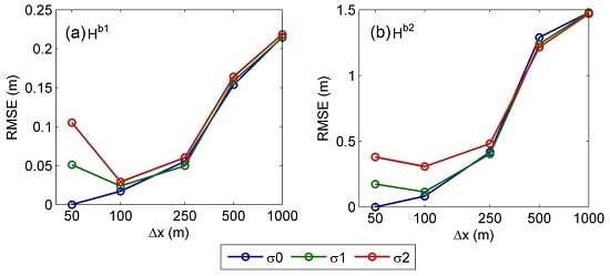
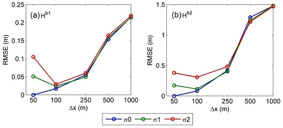
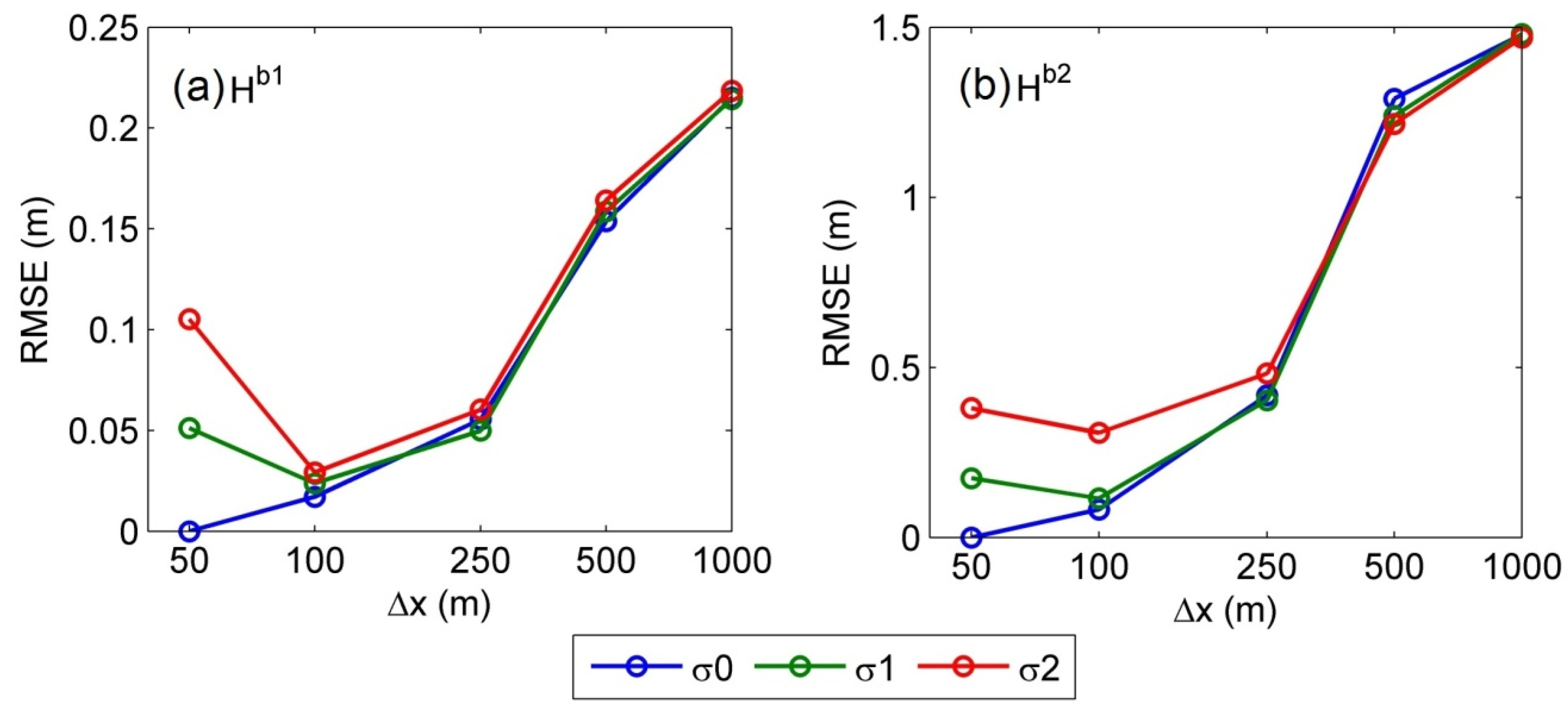
Further important insight can be gained by evaluating the relation between DEM error and grid-box size. This was achieved by plotting the water elevation RMSEs with respect to the benchmark case as a function of both DEM error and grid scale. The results, shown in Figure 5a,b for points b1 and b2 identified in Figure 3 on the right and left banks, respectively, describe a unique trade-off. High errors occur at low resolutions and coarse resolutions with a minimum error at about the 100-m grid-box scale. Greater RMSE occurs on the left bank at b2 compared to location b1 on the right bank. Furthermore, as grid-box size increases, the relative contribution of DEM error becomes negligible.

For instance, at grid-box size 1000 m, the error is associated mainly from grid box size (0.21 m at b1 (Figure 5a) and 1.50 m at b2 (Figure 5b)). Vertical accuracy is greatly reduced and therefore plays a negligible role. On the other hand, at grid-box size 50 m, the total error results mainly from the DEM error: 0.05 m for σ1 and 0.11 m for σ2 at b1 (Figure 5a) and 0.17 m for σ1 and 0.38 m for σ2 at b2 (Figure 5b). The effect of σ2 at grid box size 50 m (i.e., 0.11 m at b1 and 0.38 m at b2) is smaller than the effect of ∆x at grid-box size 1000 m (i.e., 0.22 m at b1 and 1.50 m at b2). As grid-box size increases to 500 m, from 250 m, the total error greatly increases much more than for any other grid-box size increment. Thus, based on the trade-off analysis with the given space-based floodplain elevation maps, a grid-box size of 100 m is the best choice to simulate water elevation in this study area. The results demonstrate how the trade-off between DEM error and grid-box size translates into error in model hydrodynamics. In general, the impact is associated with variability in modeled water velocities.

Figure 4. Profiles of water elevations (H) along profile a1-a2 in Figure 3 on both high water (day 28) and low water (day 62) and floodplain elevations (Z) from the 15 different models. The left and right banks (LB, RB) are separated by the main channel located at ~15 km on the profile a1-a2.

Figure 4. Profiles of water elevations (H) along profile a1-a2 in Figure 3 on both high water (day 28) and low water (day 62) and floodplain elevations (Z) from the 15 different models. The left and right banks (LB, RB) are separated by the main channel located at ~15 km on the profile a1-a2.

Figure 5. The trade-off analysis of grid-box size (∆x) and DEM error (σ) on water elevation RMSE at locations (a) b1 and (b) b2 in Figure 3, respectively.

Figure 5. The trade-off analysis of grid-box size (∆x) and DEM error (σ) on water elevation RMSE at locations (a) b1 and (b) b2 in Figure 3, respectively.

It is noted that water depth was not analyzed in this study because the focus is on space-based altimetry. Further, it was felt that the use of water elevations are likely to provide better insight because a flat water surface will be predicted regardless of the floodplain elevation associated with synthetically generated DEM errors [33].

3.2. Sensitivity of Model Water Velocity to Grid-Box Size and DEM Error

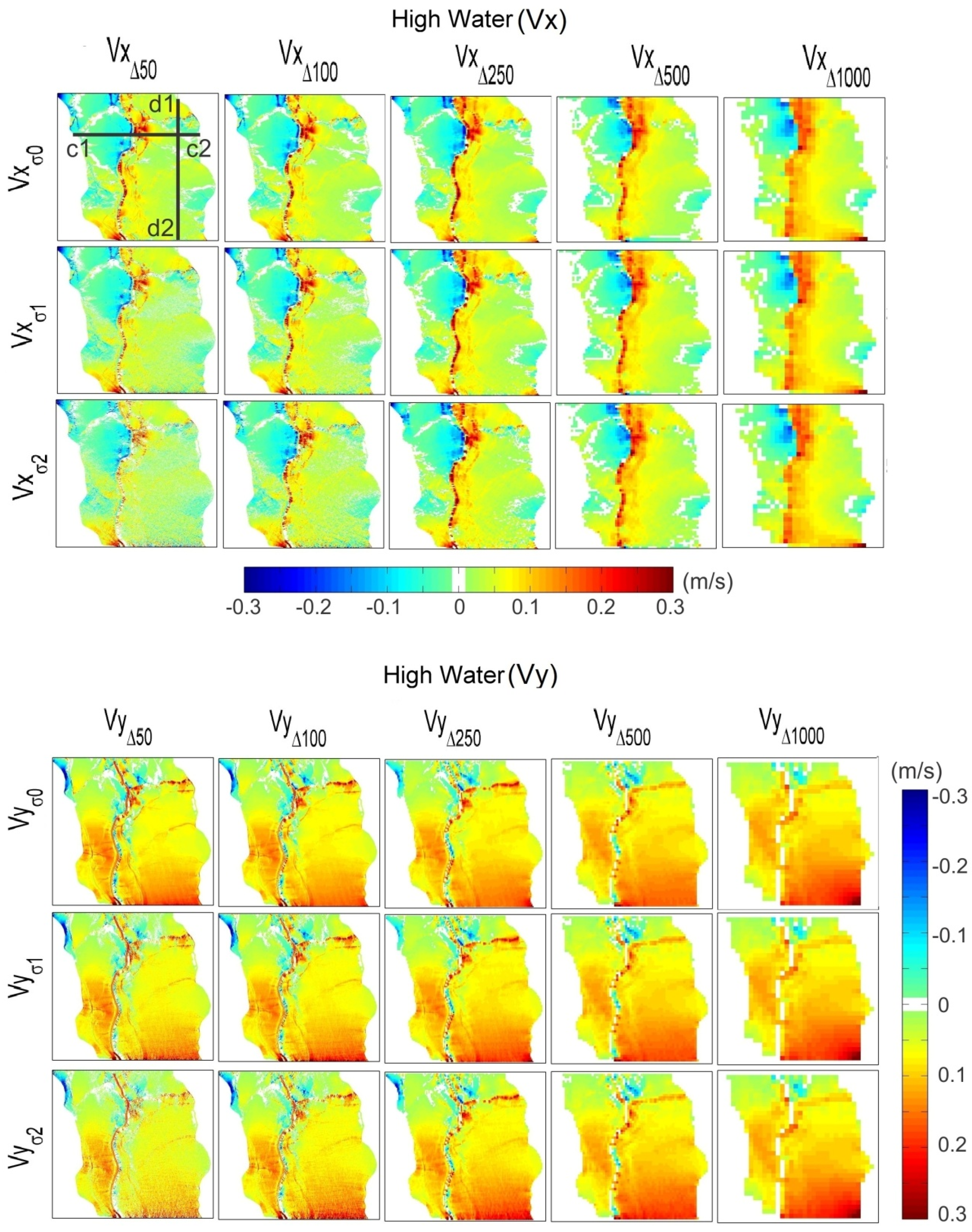
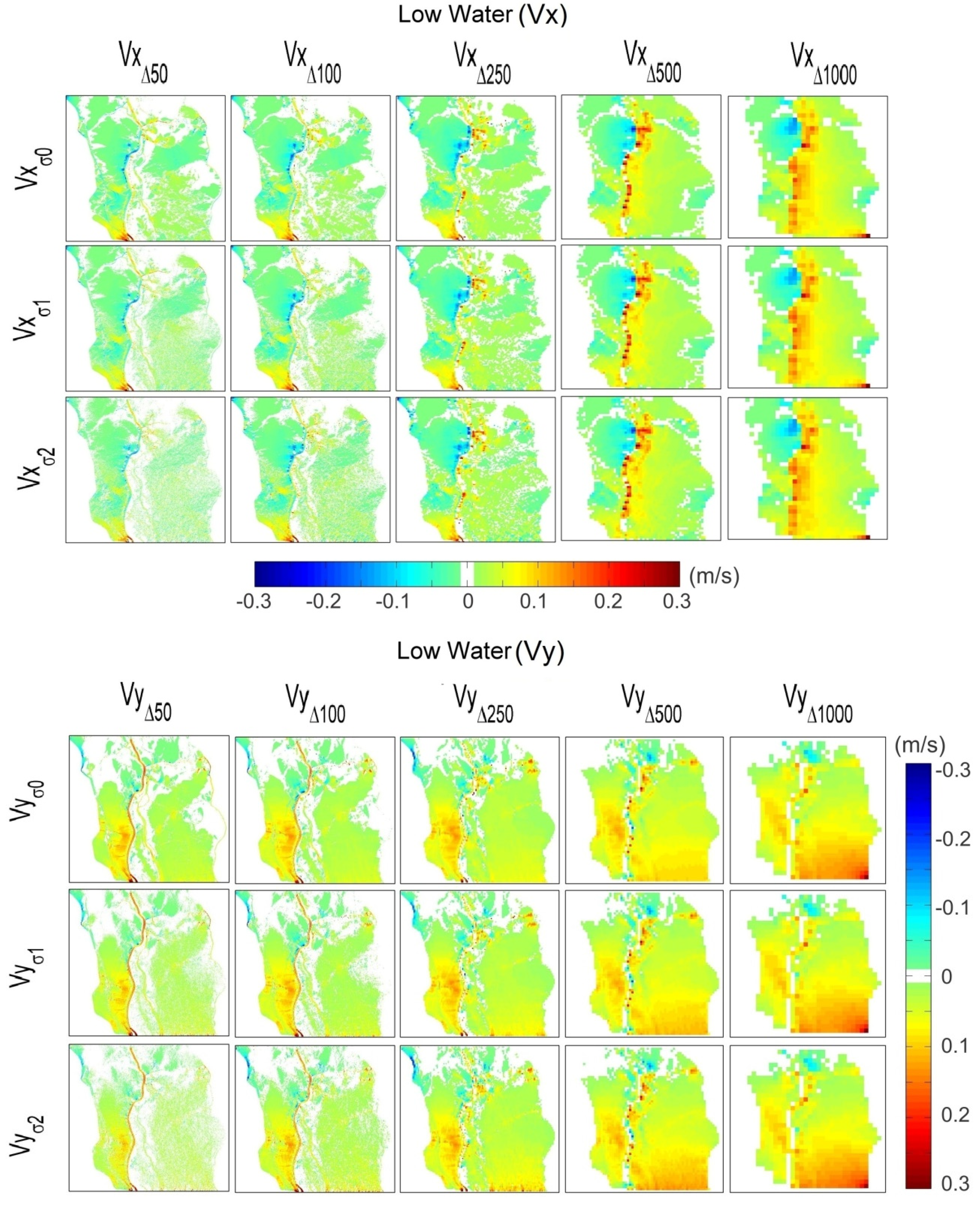
The sensitivity to modeled water velocity also was examined in a manner similar to the above. Figure 6 shows water-velocity maps in the perpendicular (Vx) and parallel (Vy) directions of the domain, where Vx is positive toward the left bank and negative toward the right bank. Vy is positive in the downstream direction and negative upstream. The two components Vx and Vy are depicted separately to better illustrate the floodwater hydrodynamics, especially in the vicinity of overbank flooding near the main channel. High-water (day 28) and low-water (day 62) periods are both shown.

The results indicate first, similar to Figure 3, the WMU boundaries are particularly evident at high water. Part of the model area shows low velocity at low water levels. In the Vx maps, most areas of high-velocity amplitudes at both high and low water are in proximity to the main stem due to overbank flooding from the main stem. In Vy, velocity generally increases linearly from upstream to downstream.

Second, as grid-box size increases, the velocity amplitude increases, demonstrating the poorer ability to represent the inundation process. Both the speed (i.e., water velocity amplitude) and the direction of water flow are affected [21]. Further, water velocities are affected by DEM error on a local scale. For the 50-m grid-box size models associated with DEM error, the slope of water velocity maps seems noisy, whereas the slope of water elevation seems very smooth. Models with grid-box sizes of 500 and 1000 m are only slightly influenced by DEM error.

Overall, the differences in water velocities among the various models are greater for high-water periods compared to low-water periods. In both Vx and Vy directions, as DEM error increases, the variability in water velocities is more clearly evident at finer grid-box size, as one might expect.

Figure 6. Water velocity maps in the direction of perpendicular (Vx) and parallel (Vy) to the main stem flow path on high water (day 28) and low water (day 62). Profiles c1-c2 and d1-d2 are used to calculate the Vx and Vy RMSEs, respectively, in Figure 7.

Figure 6. Water velocity maps in the direction of perpendicular (Vx) and parallel (Vy) to the main stem flow path on high water (day 28) and low water (day 62). Profiles c1-c2 and d1-d2 are used to calculate the Vx and Vy RMSEs, respectively, in Figure 7.

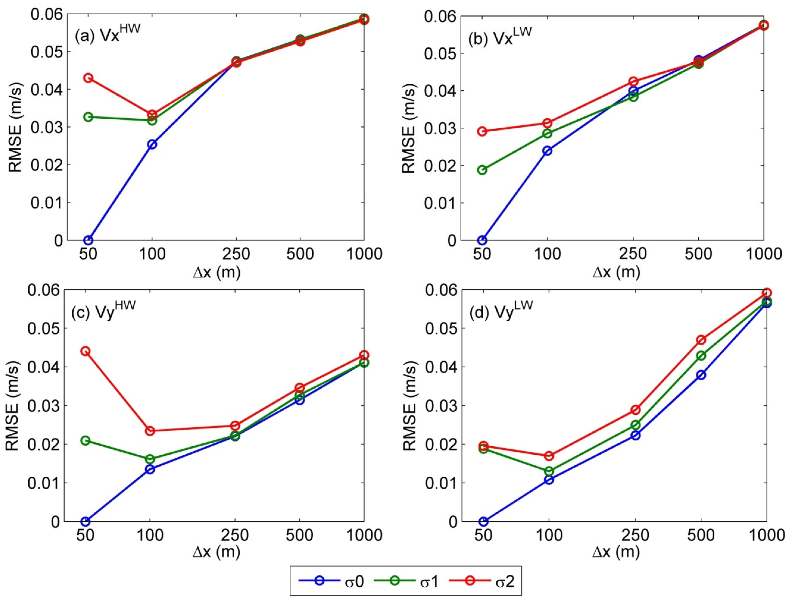
The trade-off between DEM vertical error and grid-box size, in terms of modeled velocities, is shown in Figure 7. Results are similar to Figure 5 for water elevation. As grid-box size increases, the impact ranges up to ~0.06 m/s in RMSE for both directions on both high and low waters. Overall, little impact is observed of DEM vertical error at coarser grid-box sizes 500 m and 1000 m. On high water at finer grid-box sizes 50 m and 100 m, the impact is greater than on low water. In Figure 7c, the RMSE of Vy^HW at ∆50, σ2, is greater than that of any Vy^HW at ∆1000. This suggests that the effect of DEM error on water velocity is greater than on water elevation. Similar to water elevation impacts, the trade-off analysis indicates that grid-box sizes in the range of 100 to 250 m yield the lowest overall error and are the most suitable for this particular Atchafalaya case.

Figure 7. The trade-off analysis of grid-box size and DEM error on water velocities of (a) perpendicular direction on high water, (b) perpendicular direction on low water, (c) parallel direction on high water, and (3) parallel direction on low water along profiles c1-c2 and d1-d2 in Figure 6.

Figure 7. The trade-off analysis of grid-box size and DEM error on water velocities of (a) perpendicular direction on high water, (b) perpendicular direction on low water, (c) parallel direction on high water, and (3) parallel direction on low water along profiles c1-c2 and d1-d2 in Figure 6.

4. Discussion

Although it is a simple matter to compute the reduction in relative vertical error with increasing DEM scale, the impact on floodplain flows is more difficult because the relationship between the two is a nonlinear process and regionally dependent. Results indicate that impacts on the Atchafalaya with its low-lying topography are somewhat qualitatively predictable, but not easily quantifiable without the use of the 2-D model. Increasing aggregation essentially fills the depressions and smoothes out the peaks of the terrain, making the flow less complex. However, this eventually leads to a less realistic response to the true natural topography, altering watershed boundaries and flow paths and resulting in higher RMSE. At the same time, increasing aggregation reduces the vertical DEM error that leads to improved representation and accuracy of spatially averaged flow.

The functional relation between the above two competing factors have been quantified in Figure 5 and Figure 7 in regard to elevation and velocity, respectively, using 2-D modeling. They indicate, in fact, a trade-off between vertical accuracy and observed horizontal resolution in the range of 0–1 m vertical accuracy and 50–1000 m spatial resolution, at least for this case of the Atchafalaya floodplain flows. The overall form of the trade-off, which is the same for the right and left banks, is similar, with a minimum error of about 100 m DEM grid-box scale. However, the magnitude of the trade-off is different, with the left bank showing greater overall RMSE than the right. The results further indicate that the scale of the hypothetical observations, 50 m for σ1 and σ2, is not the optimal modeling scale; rather it occurs at 100 m. Initially, the benefits resulting from increasing aggregation far outweigh the decrease in vertical error because of spatial averaging. But as aggregation increases above 500 m, the improvement from vertical error is negligible because of spatial averaging, and increasing the grid-box scale leads only to greater error.

Bank elevation plays an important role in the Atchafalaya’s floodplain hydrodynamics, as noted in previous floodplain studies [49]. Natural banks or levees divide river channels from their floodplains and during overbank flooding they limit the maximum water elevation from the main channel [49]. In this study, overbank flow was totally controlled by the 2-D raster-based DEM because the channel representation remains the same, though the DEM is varied in grid-box size and accuracy. 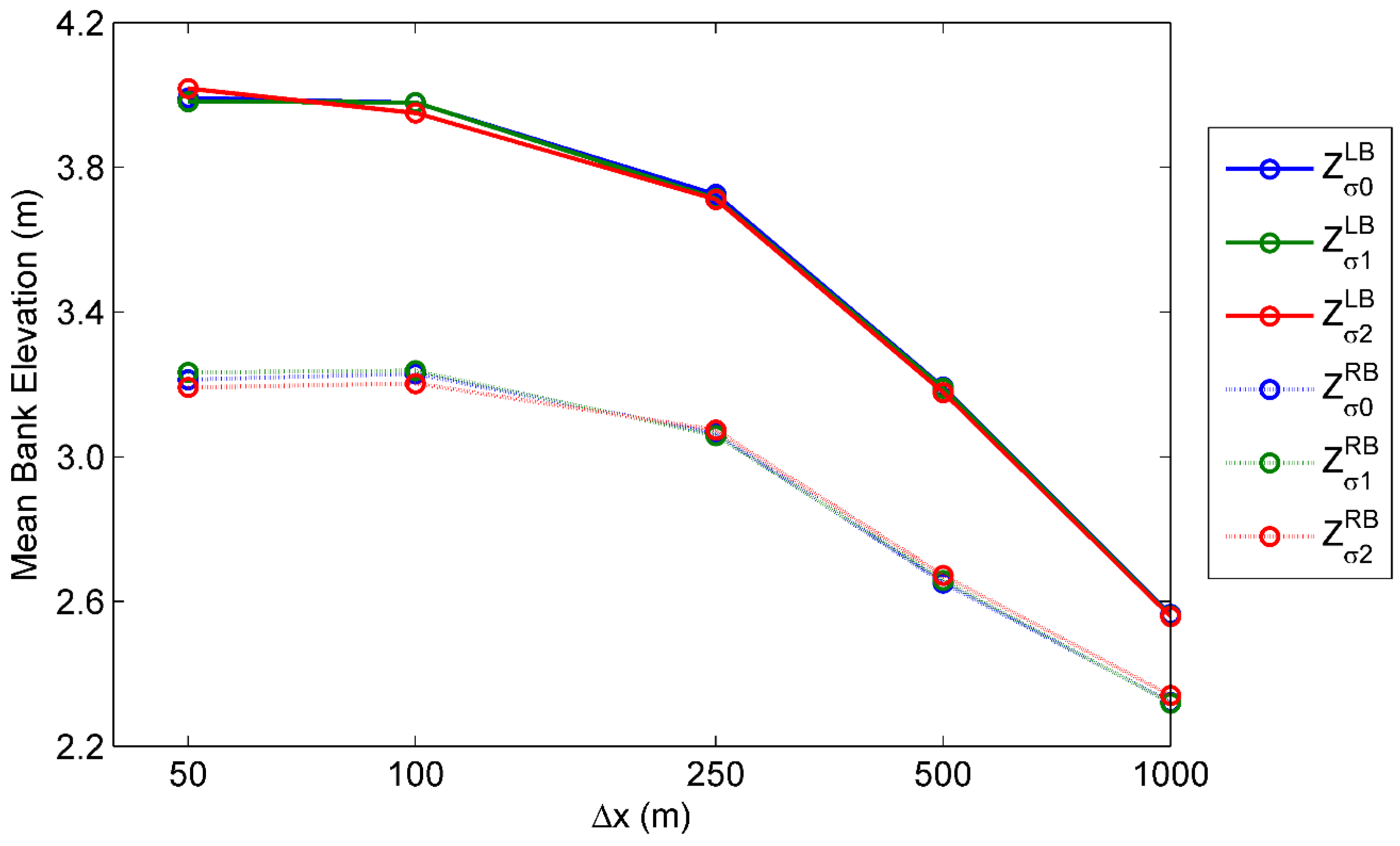As DEM error increases, bank elevation becomes noisy in Z_σ1 and Z_σ2, but the mean bank elevation remains similar to the mean of Z_σ0 at each grid-box size (Table 2). This is related to the zero mean Gaussian random error generation of synthetic DEM maps. However, as grid-box size increases, bank elevation decreases, which are clearly seen in Figure 8. This testifies that bank elevation is more affected by the effect of grid-box size than by the effect of DEM error. Overall, the left bank elevation is higher than right bank elevation in all floodplain elevation maps. However, as grid-box sizes increase, the difference between right- and left-bank elevations decreases, such that the WMU boundaries become unclear and that the distinct hydrodynamic features on each side diminish.

Table 2. The mean plus or minus standard deviation of both the left (LB) and right bank (RB) elevations in terms of grid-box size and DEM error.

unit: m	Z∆50		Z∆100		Z∆250		Z∆500		Z∆1000
	RB	LB	RB	LB	RB	LB	RB	LB	RB	LB
Zσ0	3.20 ± 1.20	4.12 ± 0.83	3.21 ± 1.17	4.06 ± 0.82	3.06 ± 1.12	3.74 ± 0.85	2.65 ± 0.93	3.19 ± 0.64	2.32 ± 0.86	2.56 ± 0.70
Zσ1	3.22 ± 1.29	4.09 ± 0.97	3.22 ± 1.21	4.06 ± 0.83	3.06 ± 1.12	3.73 ± 0.85	2.66 ± 0.94	3.19 ± 0.64	2.32 ± 0.86	2.56 ± 0.70
Zσ2	3.17 ± 1.55	4.09 ± 1.34	3.19 ± 1.21	4.03 ± 0.94	3.07 ± 1.13	3.73 ± 0.87	2.67 ± 0.94	3.18 ± 0.64	2.34 ± 0.87	2.56 ± 0.71

Table 2. The mean plus or minus standard deviation of both the left (LB) and right bank (RB) elevations in terms of grid-box size and DEM error.

unit: m	Z∆50		Z∆100		Z∆250		Z∆500		Z∆1000
	RB	LB	RB	LB	RB	LB	RB	LB	RB	LB
Zσ0	3.20 ± 1.20	4.12 ± 0.83	3.21 ± 1.17	4.06 ± 0.82	3.06 ± 1.12	3.74 ± 0.85	2.65 ± 0.93	3.19 ± 0.64	2.32 ± 0.86	2.56 ± 0.70
Zσ1	3.22 ± 1.29	4.09 ± 0.97	3.22 ± 1.21	4.06 ± 0.83	3.06 ± 1.12	3.73 ± 0.85	2.66 ± 0.94	3.19 ± 0.64	2.32 ± 0.86	2.56 ± 0.70
Zσ2	3.17 ± 1.55	4.09 ± 1.34	3.19 ± 1.21	4.03 ± 0.94	3.07 ± 1.13	3.73 ± 0.87	2.67 ± 0.94	3.18 ± 0.64	2.34 ± 0.87	2.56 ± 0.71

Figure 8. The mean of both left (LB) and right bank (RB) elevations in terms of grid-box size and DEM error.

Figure 8. The mean of both left (LB) and right bank (RB) elevations in terms of grid-box size and DEM error.

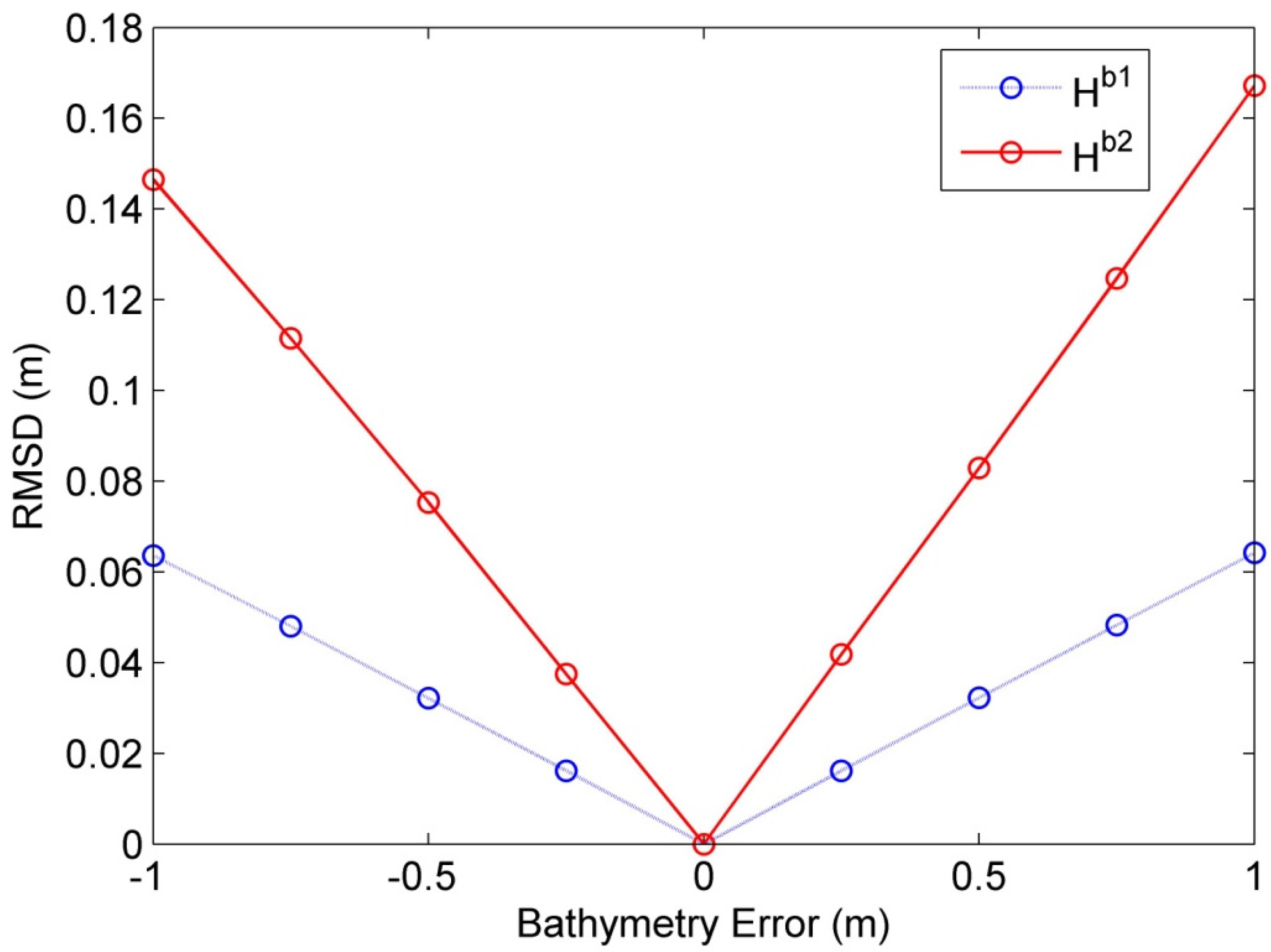
Finally, the sensitivity of the modeled water elevation to bias in channel bathymetry was investigated by changing the input bathymetry by ± 1 m in increments of 0.25 m for the benchmark 50 m case. River-width data can be measured reliably from remotely sensed data. River bathymetry has recently been estimated within ~0.5 m from water-surface elevation measurement, data assimilation, and modeling framework [10,50]. The root-mean-square deviation (RMSD) of the modeled water elevation was computed at both locations of b1 and b2 for the model period. Figure 9 shows that the bathymetry ± 0.5 m error leads to ~3 cm and ~8 cm of errors in the modeled water elevations at b1 and b2, respectively. This implies that the effect of an error in river bathymetry on the water elevation is smaller than the effect of the σ1 DEM error on water elevations (Figure 5).

Figure 9. Results of the modeled water elevations at locations b1 and b2 to uncertainty in river bathymetry, varying from −1 m to 1 m in steps of 0.25 m at the bench mark resolution 50 m.

Figure 9. Results of the modeled water elevations at locations b1 and b2 to uncertainty in river bathymetry, varying from −1 m to 1 m in steps of 0.25 m at the bench mark resolution 50 m.

The above approach assumes the use of previously calibrated Manning roughnesses for the channel and floodplain [34]. It may also be possible to recalibrate roughness with model grid-box size as different processes are forced at different topographic scales. However, the focus in this study is on model sensitivity of grid-box size and DEM error, not on adjusting Manning roughness. The infiltration into the shallow alluvial aquifer may also influence the modeling of water elevation and velocity. However, given the region, surface water and groundwater interactions are not considered relatively important in the current model sensitivity study.

As grid-box size increases, the stable time step decreases according to 1/∆x in LISFLOOD-ACC hydrodynamic model [41]. In this study, 50-m resolution allows the stable time step of 5.7 s, whereas 100-m resolution allows 11.5 s. Thus, finer resolution models require longer model run time. As for spin-up time, the model in Z_∆50,σ0 requires at least eight days to wet the whole floodplain with the shared memory Open Multi Processor (OpenMP) [50], whereas the model in Z_∆1000,σ0 requires less than one day to initialize the model.

5. Conclusions

The design parameters of satellite-based altimeters are often expressed in terms of vertical accuracy and pixel size. An approach to examining the trade-off between the two has been shown for an 1190 km²segment of the Atchafalaya floodplain. The results encompass modeling domains of O[10³] km² and greater that can employ DEMs derived from current satellite altimeters. Smaller domains that capture finer scale roughness features would require additional higher grid-box resolution analysis.

The approach was to analyze output from a numerical floodplain hydrodynamic model, using a range of synthetically generated land surface elevation maps that one might expect from upcoming space-based altimetry. The modeling approach was required because of the nonlinear relationship between input error and modeled output.

When the impacts from vertical error and DEM scale are examined separately, the results on water elevation and velocity are relatively predictable. However, when examined together in the trade-offs as in Figure 5 and Figure 7, a relationship is observed. Although magnitudes are different for the left and right banks, the form of the trade-offs is robust over the entire range of vertical accuracies and DEM scales used.

More specifically, the model sensitivity of water elevation to grid-box size and DEM error was evaluated. The modeled water elevation was more sensitive to grid-box size so that the estimate of water elevations was relatively insensitive to DEM error characteristics, especially at higher resolutions and water depth. The critical length scale appears to be related to the mean river width, 356 m. This greatly controls the overbank flooding from the main stem as the main inundation source in this floodplain.

Second, the model sensitivity of water velocity was examined in both perpendicular and parallel directions to the main stem flow direction into grid-box size and DEM error. They show more local scale features relative to water elevation in the model. The DEM error is also a major controlling factor to the model sensitivity of water velocity with the grid-box size effect. The trade-off analysis of both water error to water elevation and velocity indicates that a grid-box size of 100 m to 250 m would produce the lowest RMSE for simulating the overbank flooding. However, the results are dependent on water flow and geomorphology of the model site.

Bank elevation as a key factor characterizes the overbank flooding from the main stem into floodplain. As grid-box size increases, the crest of the floodplain levee adjacent to the main stem is smoothed out; thus bank elevation becomes lower, inducing more overbank flooding. The effect of bank elevation is more sensitive to grid-box size compared to DEM error, which is statistically determined by the mean bank elevation rather than the standard deviation.

In sum, although the study here focuses on only one basin, it offers an approach that may be applied to other riverine floodplains as a planning tool for understanding floodplain DEM requirements from future altimetry missions and as a design tool for mission planners. Such studies should include a wider range of locations, different numerical schemes and 2-D models, and diverse flooding scenarios.