Article

Evaluation of Three MODIS-Derived Vegetation Index Time Series for Dryland Vegetation Dynamics Monitoring

1
Key Laboratory of Digital Earth Science, Institute of Remote Sensing and Digital Earth (RADI), Chinese Academy of Sciences (CAS), No.9 Dengzhuang South Road, Haidian District, Beijing 100094, China
2
German Remote Sensing Data Centre (DFD), German Aerospace Centre (DLR), D-82234 Wessling, Germany
3
Department of Geography, University of South Carolina, Columbia, SC 29208, USA
*
Author to whom correspondence should be addressed.
Remote Sens. 2015, 7(6), 7597-7614; https://doi.org/10.3390/rs70607597
Submission received: 11 February 2015 / Revised: 1 June 2015 / Accepted: 2 June 2015 / Published: 9 June 2015
(This article belongs to the Special Issue Remote Sensing of Land Degradation in Drylands)

Abstract

:
Understanding the spatial and temporal dynamics of vegetation is essential in drylands. In this paper, we evaluated three vegetation indices, namely the Normalized Difference Vegetation Index (NDVI), the Soil-Adjusted Vegetation Index (SAVI) and the Enhanced Vegetation Index (EVI), derived from the Moderate Resolution Imaging Spectroradiometer (MODIS) Surface-Reflectance Product in the Xinjiang Uygur Autonomous Region, China (XUAR), to assess index time series’ suitability for monitoring vegetation dynamics in a dryland environment. The mean annual VI and its variability were generated and analyzed from the three VI time series for the period 2001–2012 across XUAR. Two phenological metrics, start of the season (SOS) and end of the season (EOS), were detected and compared for each vegetation type. The mean annual VI images showed similar spatial patterns of vegetation conditions with varying magnitudes. The EVI exhibited high uncertainties in sparsely vegetated lands and forests. The phenological metrics derived from the three VIs are consistent for most vegetation types, with SOS and EOS generated from NDVI showing the largest deviation.

Graphical Abstract

1. Introduction

Drylands cover nearly 40 percent of global land surface [1,2]. Rainfall is low and highly variable in these lands, which results in dramatic variation of temporal development and growth cycle of vegetation from year to year. Many dryland ecosystems have experienced increased threats from climate change and human-induced activities over recent decades [3,4,5,6]. Knowledge of the spatial and temporal dynamics of vegetation is essential to understand the impacts of climate change and anthropic activities on dryland ecosystems. With the capability for large spatial coverage and frequent observations, satellite data have played an important role in monitoring vegetation dynamics [7,8,9]. In particular, the spectral vegetation index dataset is known to be well-related to leaf area index (LAI), chlorophyll abundance, absorption of phtosynthetically active radiation (fPAR) and gross primary production (GPP) [10,11]. For dryland vegetation activity monitoring, time series of vegetation indices have often been used to detect variability of vegetation activity [12,13,14] and changes of vegetation phenology [15,16].
The polar orbiting Moderate Resolution Imaging Spectroradiometer (MODIS) sensor aboard the National Aeronautics and Space Administration’s Terra and Aqua platforms enable sound environmental monitoring in general and the calculation of vegetation indices, as they offer a radiometric and spatial resolution superior to that of, for example, the Advanced Very High Resolution Radiometer (AVHRR) sensor [17]. Vegetation Indices (VIs) derived from MODIS data represent improved spatial, spectral, and radiometric representations of surface vegetation conditions [18]. Among the most commonly used datasets in vegetation dynamic monitoring are the Normalized Difference Vegetation Index (NDVI) time series. However, the NDVI does have some limitations related to soil background brightness, which has an impact on the index and leads to the fact that, for similar canopy biophysical properties, different index values can be found for different soil and moisture conditions [19]. In order to overcome this problem, Huete [20] proposed a soil-adjustment factor, L, to account for the first-order, non-linear, differential radiative transfer through a canopy in the near infrared (NIR) and red regions of the spectrum, and obtained a soil-adjusted vegetation index (SAVI). After that, soil-adjusted indices such as the modified soil-adjusted vegetation index (MSAVI) and optimized soil-adjusted vegetation index (OSAVI) were developed for optimal adjustment of soil effects [21,22]. Moreover, the Enhanced Vegetation Index (EVI) was developed to optimize the vegetation signal with improved sensitivity in high-biomass regions and to provide improved vegetation monitoring through a de-coupling of the canopy background signal and a reduction in atmospheric influences [17]. The EVI has shown to be strongly linearly related and highly synchronized with seasonal eddy flux tower photosynthesis measurements in terms of phase and amplitude, encompassing a broader range in LAI retrievals [23]. The evaluation of VIs is an important and necessary process when assessing the vegetation development in different biomes. Li et al. [24] pointed out that both the NDVI and EVI derived from MODIS surface reflectance adjusted for the nadir bidirectional reflectance distribution function (NBAR) had a better accuracy than LAI in estimating the onset dates of greenness in deciduous broadleaf forest. Motohka et al. [25] found the EVI to be the most effective vegetation index for rice paddy phenology monitoring in monsoon Asia when it was compared with in situ data. Based on ground observations, Nagai et al. [26,27] examined the NDVI, EVI, and the green-red ratio vegetation index (GRVI) and found that the GRVI was the best at capturing the seasonal changes in photosynthetic capacity, as green and red reflectances are strongly influenced by changes in leaf pigments. Due to its insensitivity to background reflectance and being a better predictor of Gross Primary Productivity, a 2-band EVI (EVI2) has been found to be a better index than the NDVI for monitoring vegetation phenology and activity across a variety of ecosystems [28]. Wu [29] developed a new Generalized Difference Vegetation Index (GDVI) to characterize land of dryland environment.
For the diverse arid and semi-arid environment, the ability of NDVI time series to capture the seasonal and inter-annual variability has been confirmed in vegetation communities such as desert grassland, desert, woodland, savanna and shrub-steppe [12]. The SAVI, which is closely related to NDVI and can minimize the effect of soil brightness, has been used to record vegetation development for the semi-arid ecosystem in northwestern Mexico [30,31]. In addition, the MODIS-derived EVI and NDVI showed a strong linear relationship with gross primary production comparing with in situ flux measurements at a station located in the semi-arid environment of Sahel [32,33]. Despite these applications, the detection results of VIs in arid and semi-arid lands were suggested to be interpreted with caution due to the high uncertainties of VIs in sparsely vegetated areas [14,34], heterogeneity landscape structure and complex vegetation composition [16,35]. To address these issues, the main objective of this study is to evaluate three MODIS-derived vegetation index products—in particular, concerning their suitability for monitoring vegetation dynamics in the arid environment of the Xinjiang Uygur Autonomous Region (XUAR), China. We derive the NDVI, SAVI, and EVI from the MODIS reflectance data and compare their spatiotemporal variation across the study region and along transects. Since the spring and autumn phenological transitions are important factors regulating plant growth and carbon sequestration [36], two phenological metrics, the start of the season (SOS) and end of the season (EOS), are mapped from the VI time series and compared regionally. The suitability of the VIs for vegetation dynamic monitoring in drylands is discussed in detail.

2. Study Area and Data
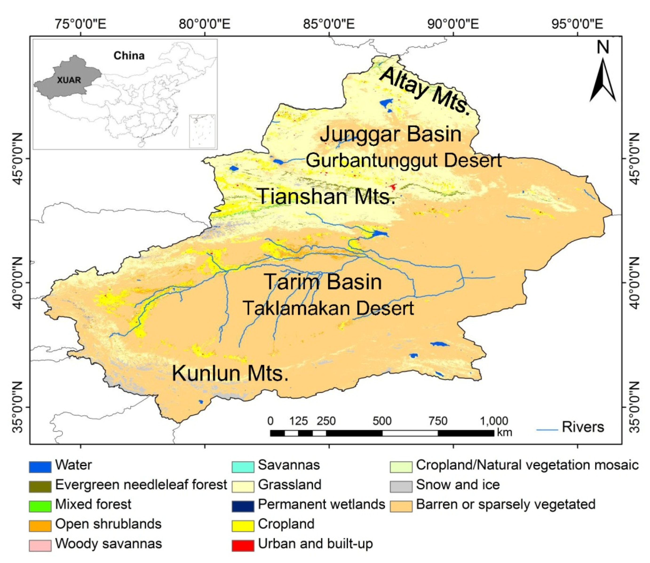
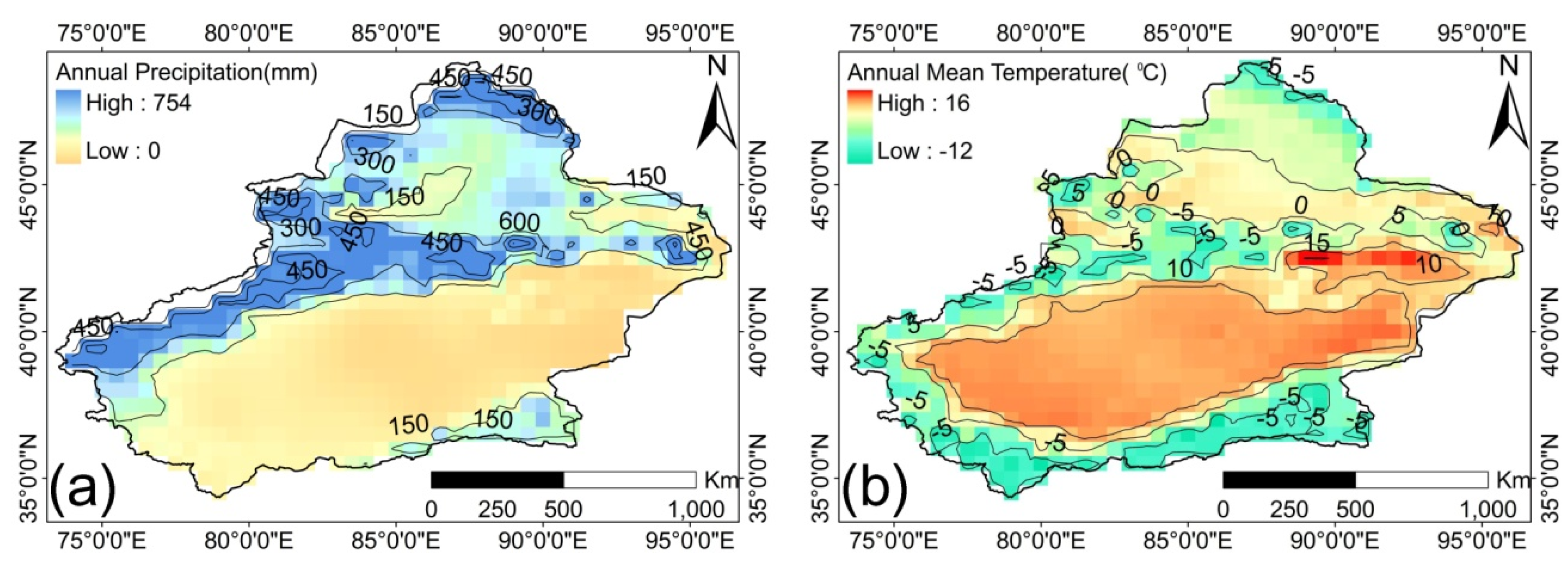
2.1. Study Area

The Xinjiang Uygur Autonomous Region (XUAR) is the largest autonomous region in China, covering 1,660,000 km2, which is more than one-sixth of China’s territory. Due to the variations in topography and climate, the land cover types vary greatly in the XUAR as shown in Figure 1. The Junggar Basin and the Gurbantunggut Desert lie between the Altay and Tianshan Mountains. The Tarim Basin and Taklamakan Desert are situated between the Tianshan and Kunlun Mountains. The entire area can be divided to northern and southern parts by Tianshan Mountains. The land is mainly covered by grassland and sandy desert [37,38,39]. Forest scatters within high mountains and along rivers. Oasis landscapes ranging from small to moderate in size (0.01–15,000 km2) have developed in river deltas, alluvial-diluvial plains and the edges of diluvial-alluvial fans [40]. Agricultural land and human settlements are found in the oases as these provide stable water supply in this arid region.
Located in the hinterland of Eurasia continent, it has a variable arid to semi-arid continental climate with annual precipitation of 100–200 mm and mean annual temperature of 10–15 °C [41]. The annual precipitation is unevenly distributed with a general decreasing pattern from northwest to southeast across XUAR (Figure 2). The annual precipitation of the northern XUAR is 210 mm while the southern XUAR has an annual precipitation of 100 mm.The mean July temperature is 27.1 °C and the mean January temperature is −17.1 °C [41]. The areas within high mountain ranges have a typical mountain climate, which is characterized by long, cold winters and short, hot summers. The growing season for vegetation extends from March to November in XUAR. Typical crops planted in these areas include wheat, cotton, corn, and rice, as well as vegetables and fruits such as sugar-beet and melon [42].
Figure 1. Geographical location and land use/cover of the XUAR. The land use map is extracted from MODIS land cover type product [39].
Remotesensing 07 07597 g001
Figure 2. Spatial distribution of (a) annual precipitation and (b) annual mean temperature in the XUAR in 2012. The climate data is from the monthly meteorological data records of the National Meteorological Information Centre, China Meteorological Administration.
Remotesensing 07 07597 g002

2.2. Data

The MODIS Surface-Reflectance Product (MOD09A1) provides an estimate of the surface spectral reflectance values at 500 m resolution in a gridded format using a sinusoidal projection. Each MOD09A1 pixel contains the best possible observation during an 8-day period, selected as the one with large observation coverage, a low viewing angle, an absence of clouds or cloud shadow, and aerosol loading [43]. The MOD09A1 products over the XUAR for the period 1 January 2001 to 31 December 2012 were extracted. The study area can be fully covered by six MODIS data tiles. To generate a 12-year VI time series, a total of 3312 data tiles were downloaded and processed, covering the entire XUAR region.
The MODIS 500 m land-cover product (MCD12Q1) was used to identify primary land covers in the study area. With the International Geosphere-Biosphere Programme (IGBP) land-cover legend [39], the MODIS product of 2012 was downloaded and served as base information in this study.

3. Methods

The data processing strategy includes the following steps. The MOD09A1 data tiles were first mosaicked, reprojected using the MODIS Reprojection Tool and masked with the XUAR boundary at the pre-processing step. Per-pixel QA information in MODIS products allows for removal of most contamination of the NDVI signal related to clouds, aerosol and snow. The time series of vegetation indices, including NDVI, EVI and SAVI, were then calculated from 2001 to 2012. The spatiotemporal patterns of monthly and annual variation were compared for different VIs. Based on the smoothed VI time series, phenological metrics were detected. The regional phenology detection results over the study area were finally generated and compared.

3.1. VI Derivation

The NDVI is defined by [17]:
NDVI = ( NIR RED ) ( NIR + RED )
where NIR is the reflectance value in the near infrared band, and RED is reflectance in the red band, respectively. For the MOD09 data, band 2 represents the near infrared reflectance (871–876 nm) and band 1 represents the red reflectance (620–670 nm).
The SAVI is defined by [20]:
SAVI = ( NIR RED ) ( NIR + RED + L ) × ( 1 + L )
where L is the soil brightness correction factor. The value of L varies with the amount or cover of green vegetation: in very high vegetation regions, L = 0; and in areas with no green vegetation, L = 1. Generally, a value of L = 0.5 works well in most situations and is the default value used. When L = 0, then SAVI = NDVI. We set L = 0.5 as suggested in our study.
The EVI is defined by [17]:
EVI = G × ( NIR RED ) ( NIR + C 1 × RED C 2 × BLUE + L )
where G = 2.5, C1 = 6, C2 = 7.5, L = 1. BLUE is the reflectance in the blue band. The coefficients 2.5 and 1 represent the gain and canopy background, respectively [17]. The atmospheric influence on the red band is corrected using the blue band and the coefficients 6 and 7.5, respectively. Band 3 of MOD09 data represents blue band reflectance (459–479 nm).

3.2. VI Means and Variability

The mean monthly VI was calculated from the monthly VI data based on the 2001–2012 time series. For every pixel, the monthly 12-year arithmetic mean ( VI ¯ m ) was calculated using Equation (4), with n being the number of years and VIm the monthly VI value.
VI ¯ m = 1 n 1 n VI m
The mean annual VI ( VI ¯ a ) was calculated accordingly from the annual sums of the VI. To better represent vegetation growth condition, only VIs in the growing season (from March to November) were used for mean annual VI and variability calculation.
The deviation (DVIi) from the 2001–2012 mean annual VI at a given spatial location for a certain year i was calculated as:
DVI i = VI i VI ¯ a
In addition, the relative annual VI deviation (rDVIi) was derived. This describes the deviation as a percentage from the mean annual VI:
rDVI i = DVI i · 100 VI ¯ a
The mean annual VI variability ( VVI ¯ ) was derived with the relative annual VI deviation (rDVIi), with n being the number of years:
VVI ¯ = 1 n 1 n | rDVI i |

3.3. Phenological Metric Detection

The software TIMESAT is a common tool for time series data analysis [44]. Despite the uncertainty of VI time series ,the curve fitting method of TIMESAT has a good performance of noise reduction and the maintenance of signal integrity and achieved consistent results from the three VIs for most vegetation types [45,46]. In our study, TIMESAT was used to smooth the time series of VIs as well as to estimate the phenology metrics for the study area. Local Gaussian-type functions were fit to data in intervals around maxima and minima of the time-series. In this paper, two phenological metrics, namely the start of the season (SOS) and end of the season (EOS) were mapped and analyzed for all VI time series. The phenological metrics that were detected, and their definitions, are listed in Table 1.
Table 1. Phenological metrics and their definitions [44].
MetricAbbreviationDefinition
Start of the seasonSOSTime for which the left edge has increased to 30% of the seasonal amplitude measured from the left minimum level.
End of the seasonEOSTime for which the right edge has decreased to 30% of the seasonal amplitude measured from the right minimum level.

4. Results

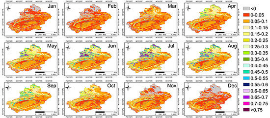
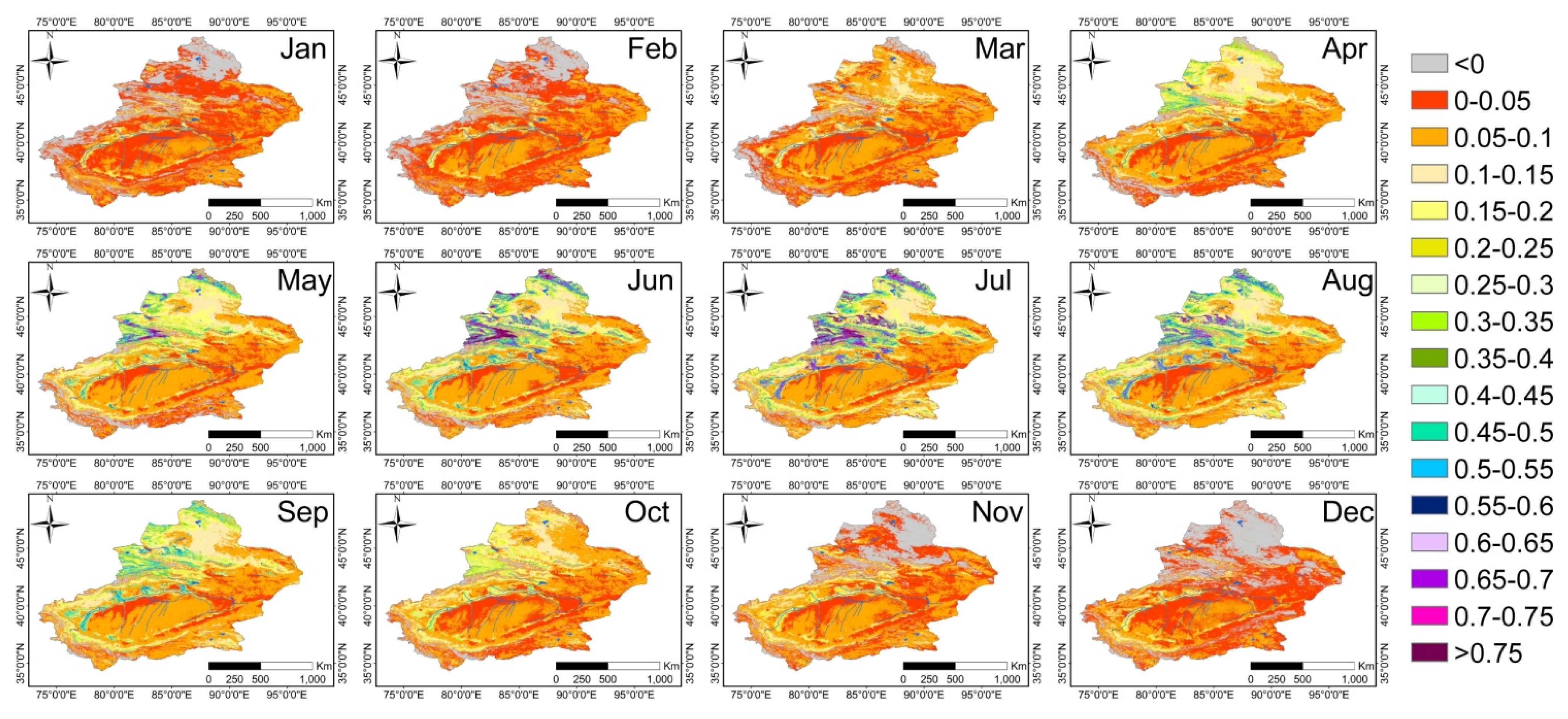
4.1. Mean Monthly VI

Figure 3 depicts the mean monthly NDVI from January to December for 2001–2012. The mean monthly VI demonstrates the growth cycle of different vegetation types throughout the year. The monthly VI indicates that the beginning of vegetation development starts between March and April in XUAR. In October, vegetation starts to be senescent throughout the region. From December to February only low VI values are observed.
Figure 3. Seasonal dynamics of the mean monthly NDVI from 2001–2012. Average VI values were calculated for each month for the period 2001–2012.
Remotesensing 07 07597 g003
The temporal evolution of vegetation index reflects the growth pattern for different vegetation types. For instance, agricultural areas do not show high vegetation activity before April, while the natural steppe at the same latitude has already started green-up in March. The growth of forests in the Altay Mountains in the north of XUAR is hindered by low temperatures before May. The maximum vegetation index is reached in June throughout the region for most vegetated areas. For the shrublands and grasslands in the Jungar Basin, the VIs drop sharply in December and then increase again by April of the following year. The sharp decrease in the vegetation index is mainly caused by the dormancy of vegetation.

4.2. Mean Annual VI and Variability

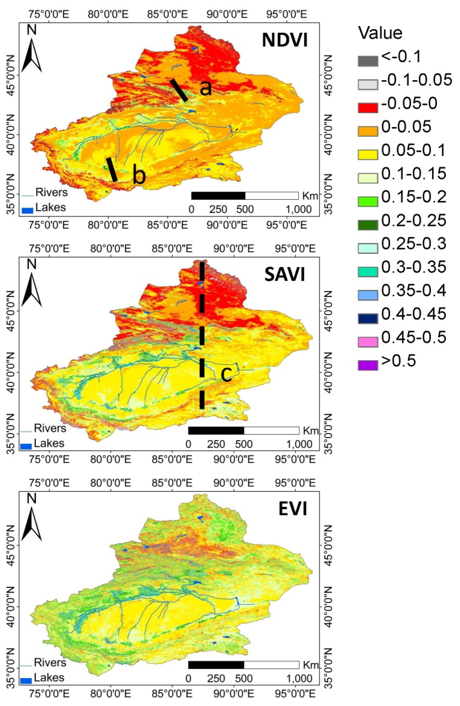
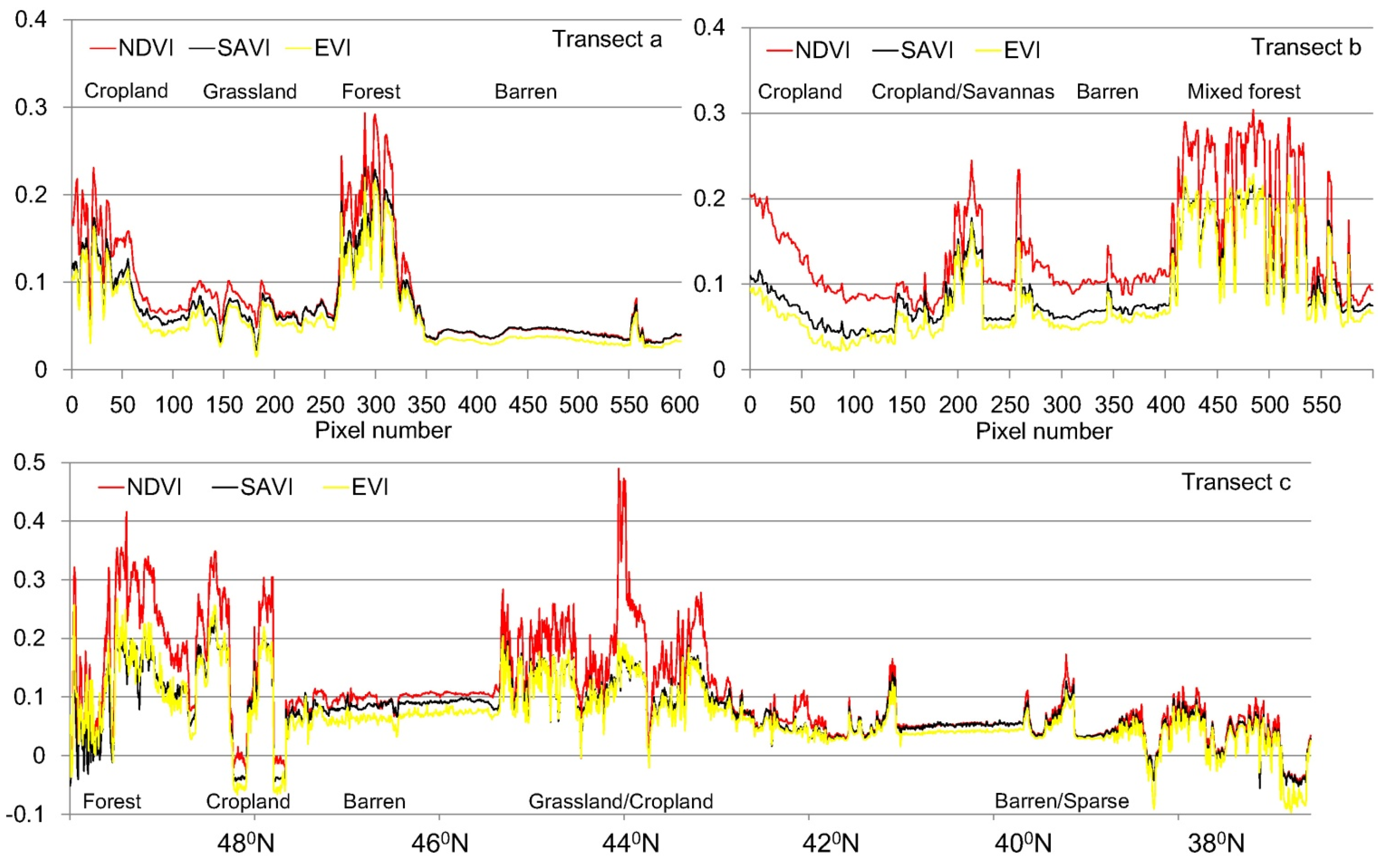
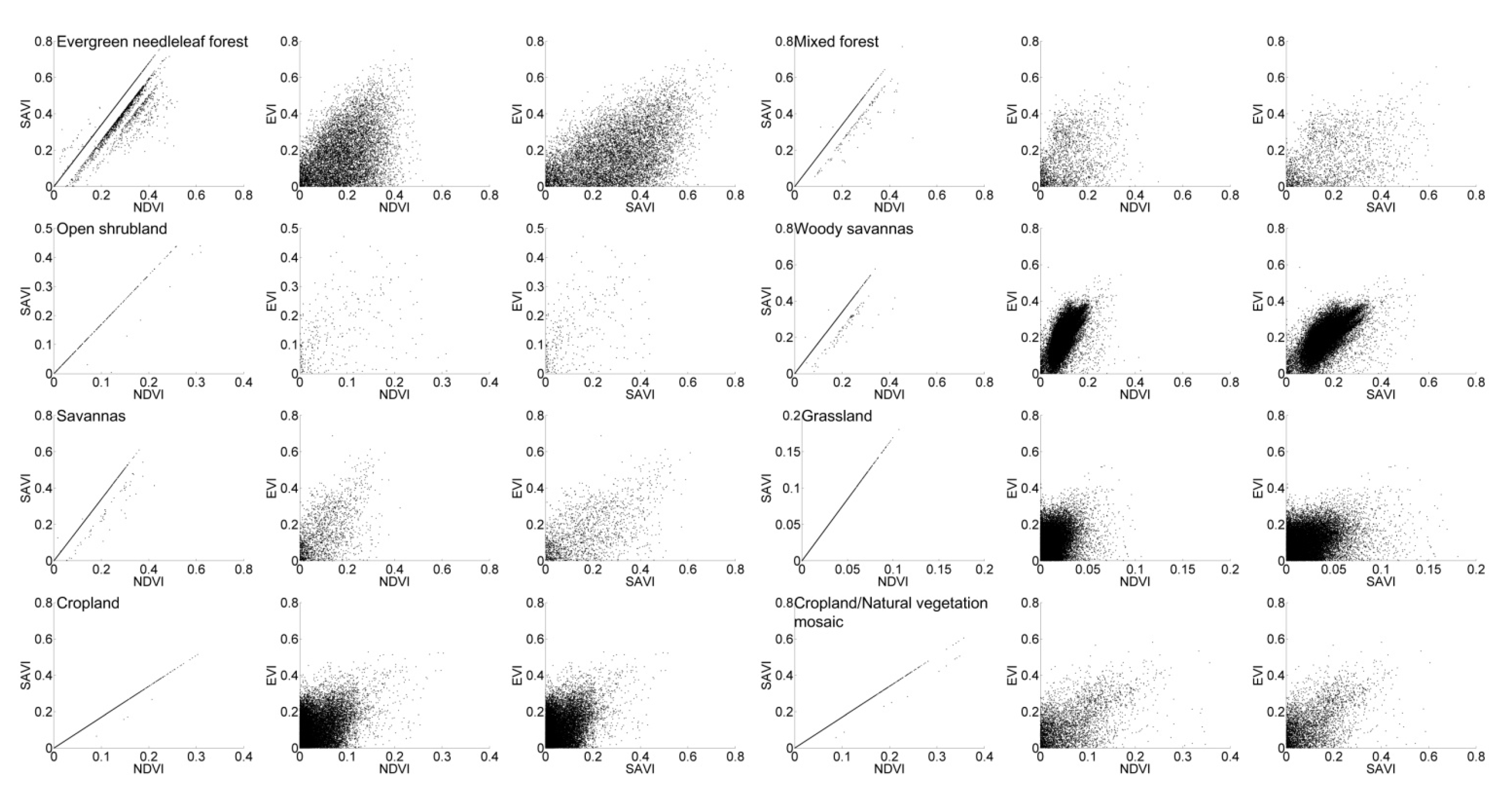
4.2.1. Mean Annual VI

The annual mean of the NDVI, SAVI, and EVI for the XUAR in 2001–2012 are presented in Figure 4. The annual mean VI images exhibit similar spatial patterns for vegetation conditions, but with varying magnitudes. All VIs depict a spatial pattern with northern and central Xinjiang having high VI values and the eastern and southern areas having low values.
Figure 4. Spatial distribution of average annual (a) NDVI; (b) SAVI; and (c) EVI derived from MODIS 8-day surface reflectance data for 2001–2012 for the XUAR. The three transects are marked in the figure.
Remotesensing 07 07597 g004
The spatial variation of annual mean VI across the northern and southern XUAR corresponds with regional climate conditions (Figure 2). With higher rainfall in northern XUAR, the forests, grasslands, and agricultural land have better growing conditions and longer growing seasons. In contrast, relatively short growing seasons are found along the Kunlun Mountains in the southern XUAR. The growth of vegetation is limited by low precipitation throughout the year in this zone. The NDVI image shows higher values than SAVI and EVI images in most areas. Over dense forests and grasslands distributed around the Tianshan Mountains and northern Altay Mountains, NDVI exhibits high mean annual values comparing with SAVI and EVI images.
In order to illustrate the spatial differences between the NDVI, SAVI and EVI in distinctive ecoregions, three transects were sampled within the annual mean VI images (marked in Figure 4a,b). Each transect crossed sparsely to densely vegetated regions in order to encompass a wide range of VI values. The land cover types along the transects included cropland, grassland, forest, and barren desert. Comparing the profiles, similar trends can be found between the VI profiles (Figure 5). However, larger data ranges were observed in the NDVI profiles than the SAVI and EVI profiles.
Figure 5. Profiles of mean annual VIs for 2001–2012 along the three transects. (a) Ecoregion gradient passing several oases; (b) elevation gradient; (c) variation along 87°E longitude. The locations of the three transects are marked in Figure 4.
Remotesensing 07 07597 g005
Transects a and b start in the northwest and end in the southeast and are about 300 km long. Transect a starts in the agricultural land near the Ebinur Lake in the north. It extends to the sparse grassland and crosses the forests of the Tianshan Mountains, which are areas with very high VI values. The transect ends in sparsely vegetated areas. Transect b starts from the crop areas of an oasis in the north, crosses a mixture of sparse vegetation and agricultural land located in the desert. The transect ends in the foothills of the Kunlun Mountains, where the mixture of natural vegetation types in small patches causes strong oscillation of the mean annual VI. The transect c follows the 87°E longitude line from north to south and is about 1460 km long. The northern part of the transect is characterized by a mixture of grassland and forest, where EVI and SAVI show variation while NDVI has little variation. In the zone between 47°N and 45°N the VI values are lower and show a rather smooth behaviour. This region is characterized by homogeneous land cover that is mainly grassland with small areas of bare grounds and open shrublands. The higher values between 45°N and 41°N correspond to the agricultural land, forests, and steppe along the Tianshan Mountains. The VI of the grassland between 41°N and 39°N, located in the Taklamakan Desert, is significantly lower than that of the grassland between 47°N and 45°N, since this area has an extremely arid desert climate and the vegetation is very sparse. The transect line crosses a transitional zone with open shrubland, cropland, and grassland and reaches the Kunlun Mountains south of 39°N. In this zone, the climate is extremely cold and dry with primary land covers of gravel desert, alpine desert and alpine desert steppe.
The relationships between the VIs for main vegetation types in the MODIS land cover product are depicted in Figure 6 and summarized in Table 2. All of the VIs show significant linear relationships between each other (p < 0.05) with varying correlations in different vegetation types. There is a strong linear relationship (R > 0.94) between the NDVI and SAVI for each vegetation type. The highest correlations were found in areas of cropland and grassland. NDVI and SAVI have a moderate correlations (R = 0.55) with EVI in areas of woody savannas. For grassland and mixed forest, the relationship between NDVI, SAVI and EVI are weakest (R = 0.29 to 0.40). The SAVI and EVI have a stronger linear relationship than NDVI with EVI.
Table 2. The Pearson’s correlation coefficients of mean annual VIs for 2001–2012 for different vegetation types.
Vegetation TypeNDVI and SAVINDVI and EVISAVI and EVI
Evergreen Needleleaf Forest0.94220.40930.4916
Mixed Forest0.97730.36750.4032
Open Shrubland0.98670.41630.4585
Woody Savannas0.99490.65040.6630
Savannas0.98490.54470.5717
Grassland0.99990.28860.2886
Cropland0.99980.40950.4096
Cropland/Natural Vegetation Mosaic0.99870.51490.5196
Figure 6 shows the scatter plots between the mean annual VIs over the 2001–2012 period. The relationship between EVI and NDVI and SAVI exhibited a high scattering of sampling points. The EVI variations corresponding to each SAVI and NDVI are mostly caused by the variation of the blue band, since EVI values rely on the blue reflectance in addition to red and NIR. For evergreen needleleaf forest, mixed forest, woody savannas and savannas, scattering samples values are observed comparing NDVI with SAVI and EVI at value ranges from 0.2 to 0.6.
Figure 6. Scatter plots of the mean annual VIs for the years 2001–2012 among the three VIs for different vegetation types.
Remotesensing 07 07597 g006

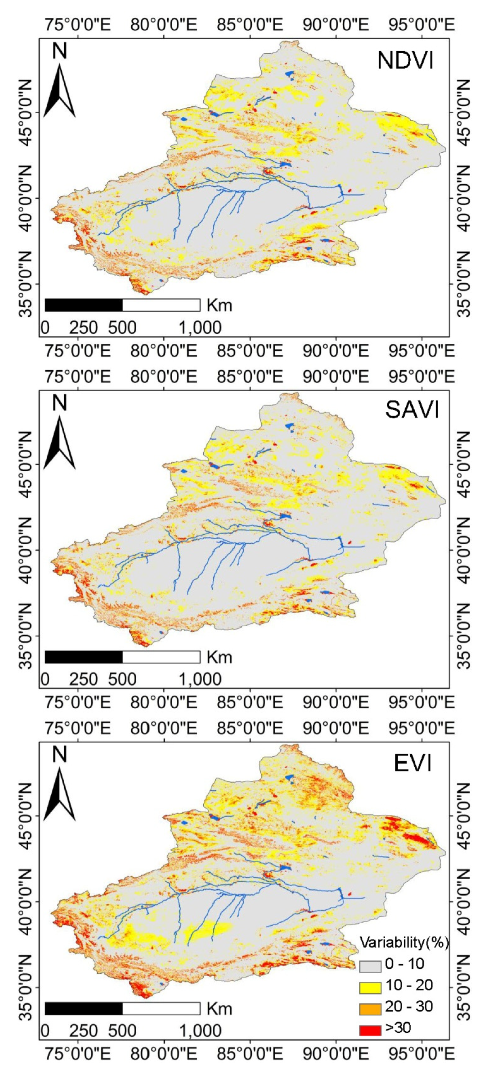
4.2.2. Mean Annual VI Variability

The mean annual VI variability for the 2001–2012 period is displayed in Figure 7. The figure illustrates spatial patterns showing how the mean annual VI varies from year to year.
Figure 7. Mean annual VI variability for 2001–2012 for the XUAR. Mean percentage variability was calculated as the mean of the absolute percentage deviations from the mean annual VI for 2001–2012.
Remotesensing 07 07597 g007
The statistical results of the variability are listed in Table 3. The results indicate that 70%–80% of the area of the XUAR has low annual VI variability (<10%) and 20%–30% of the area has variability higher than 10%. In particular, 10%–15% of the area shows variability between 17% and 24%, and only 3%–6% of the area varies by more than 30%. Comparing the three variability maps quantitatively, the EVI image shows the highest variability (Table 3). Therefore, the EVI time-series captures larger inter-annual variability from 2001 to 2012 for the entire XUAR comparing with NDVI and SAVI. Considering the scarcity of vegetation in the Taklamakan desert, the high variability observed only from EVI data in this area might be caused by the variation in soil background property.
Table 3. Percentage of mean annual VI variability for 2001–2012 for the XUAR.
PercentageNDVISAVIEVI
0%–10%77.4478.9169.16
10%–20%15.9314.7418.89
20%–30%3.242.935.67
>30%3.393.426.28

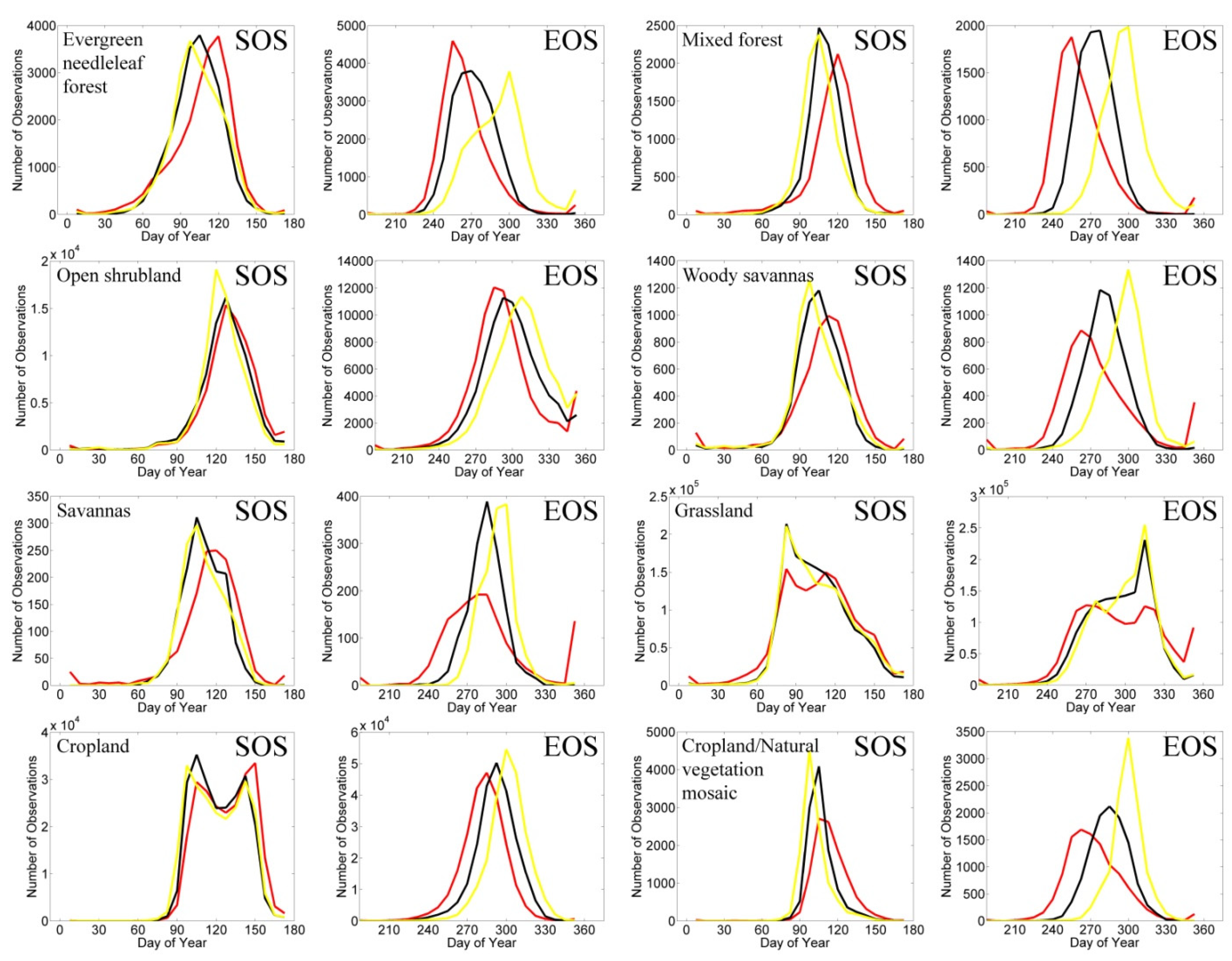
4.3. Phenological Metric Detection

Based on the three VI time series, the SOS and EOS over the XUAR are mapped for the period 2001–2012. Their mean and standard deviation (SD) from the three VI datasets for each vegetation type are summarized in Table 4. The standard deviation of SOS ranges from 11.9 days to 37.6 days. The standard deviation of EOS ranges from 13.3 days to 47.0 days. The EOS from NDVI shows greater deviation than SAVI and EVI except for evergreen needleleaf forest. The SOS from NDVI time series show greater deviation than SAVI and EVI except for cropland.
Table 4. Mean day of year (DOY) and standard deviation (SD) of phenological metrics detected from VIs for 2001–2012 for the XUAR.
SOSNDVISOSSAVISOSEVIEOSNDVIEOSSAVIEOSEVI
MeanSDMeanSDMeanSDMeanSDMeanSDMeanSD
Evergreen needleleaf forest117.429.1112.821.4113.024.4277.326.3284.920.2306.328.0
Mixed forest127.026.6119.515.0114.915.8274.328.1286.815.2311.319.3
Open shrubland142.227.6137.722.7135.620.9308.035.7315.128.0324.128.0
Woody savannas120.237.6113.824.2112.526.8288.445.1294.724.1310.626.6
Savannas125.632.4120.716.3120.917.4297.747.0298.014.4307.614.3
Grassland117.735.4115.928.0117.129.0311.242.6311.629.3314.428.2
Cropland139.121.9133.320.7132.522.1296.519.6306.418.0316.117.1
Cropland/natural vegetation mosaic124.617.8116.711.9111.612.0285.925.9298.816.4314.013.3
Histograms of the two phenology metrics for different vegetation types are illustrated in Figure 8. Despit the shift of peak, the histogram distributions of SOS and EOS from three VIs are in agreement. Obvious bimodal distributions are displayed for the SOS of grassland, SOS of cropland and EOS of cropland. The bimodal distributions of SOS and EOS of cropland indicate different phenological patterns of different crop types. Due to the influence of bare soil on vegetation index [47], grasslands of different densities may show inconsistent green-up behaviours, which causes the bimodal distributions of SOS. Discrepancies from three VIs are observed for the SOS of grassland, EOS of evergreen needleleaf forest and EOS of grassland. For grassland, SOSNDVI has a large peak and secondary peak at DOY80 and DOY110, while SOSNDVI has two similar peaks. Similar discrepancies are observed from EOS of grassland. For evergreen needleleaf forest, EOSEVI has bimodal distribution compared to unimodel distribution of EOSNDVI and EOSEVI. The values distributed near the tail of the histogram indicate overestimations in the EOSNDVI of evergreen needleleaf forest, mixed forest open shrubland, woody savanna, savanna and grassland.
Figure 8. Histograms of the two phenological metrics detected from VI time series for each vegetation type for 2001–2012 for the XUAR. The red line denotes NDVI, the black line denotes SAVI and the yellow line denotes EVI.
Remotesensing 07 07597 g008

5. Discussion

5.1. VI Variability

The existence of cloud causes a drastic decrease of VI values. In particular, NDVI is more sensitive to atmopheric effects than EVI. The contamination of residual clouds leads to the large variation in NDVI values as we can see in Figure 5. Though we used the cloud mask to reduce cloud effects on per-pixel surface reflectance, there are still uncertaities in the MODIS cloud mask [48,49]. The inclusion of cloud and aerosol corrupted EVI has been found to misidentify the vegetation changing trend [50]. Therefore, the usage of quality assessment information for atmospheric and cloud screening is essential for the reliability of vegetation change detection results. Additional masking may be required to exclude contaminated pixels [51]. These indicate that uncertainties can be caused when using NDVI time series for vegetation variability detection.
High VI variability (>30%) can be observed in mountain areas (Figure 7). This might be caused by the highly variable meteorological conditions in this mountainous environment. Medium VI variability (10%–30%) exists in several grassland-dominated areas, as well as in the agricultural areas in the northern XUAR. The variability here might be caused by a mixture of small crop fields and changing agricultural practices. The zones with semi-arid to arid conditions in the Taklamankan desert and Gurbantunggut desert show very stable mean annual VI within the observed time period. In particular, EVI exhibits more variability than NDVI and SAVI for the sparsely vegetated areas. For these areas, the soil background is mainly composed of dry sand. NDVI has been reported to be susceptible to the spectral influence of soil texture and moisture in gaps between vegetation for desert grass and desert shrubland [52,53]. The high annual variability detected from EVI may be related to variation of soil background at low VI levels.

5.2. Phenological Metric Detection

Using the curve-fitting method of TIMESAT with the same the seasonal amplitude thresold (30%), different dynamic ranges of VIs can cause a shift of phenology detection results, as we can see in Figure 8. Despite the uncertainty of VI time series, the application of TIMESAT achieved consistent results from the three VIs for most vegetation types. Agreeing with past studies [12,30], the three VIs in this study proved their effectiveness for phenological metric detection in dryland enviroment.
However, there are still some discrepencies in phenology detection results. The uncertainty of EOS detected from MODIS VIs in our study is higher than SOS (Table 4), which is in agreement with previous studies [47,54]. The largest deviation of phenological metrics and the overestimation of EOS are observed from NDVI time series. Due to its sensitivity to soil background and atmospheric conditions, it exhibited high levels of variation. The disagreement among histogram distributions of phenological metrics from the three VIs can be caused by their different sensitivities to the variation of soil background. Similarly, Walker et al. [16] revealed the spatial variability of land surface phenology extracted from NDVI is higher than EVI in dryland areas in Arizona, USA. The discrepancy of the peak greenness from EVI and NDVI has been attributed to their different sensitivities to the physiological characteristics of vegetation types [16].
In order to better assess the suitablity of VIs for phenological detection in dryland enviroment, more detailed information is needed. Verification of satellite-extracted phenology metrics with CO2 measurements of flux tower footprint or in situ VI measurements will be helpful to our understanding of ecosystem processes over arid lands [55,56]. The inaccessibility of in situ data precludes further analysis in our study. In addition, we only compared three commonly used VIs in our analysis. The effectiveness of other vegetation indices such as EVI2, MSAVI and OSAVI and combined usage of these indices for vegetation dynamic investigation in arid and semi-arid dryland can be addressed in further studies.

6. Conclusions

Three vegetation indices derived from MODIS data were assessed in vegetation dynamic monitoring in the XUAR, China. The annual mean VI images exhibited similar spatial patterns of vegetation conditions with varying magnitudes. NDVI, SAVI and EVI were all related to each other with varying correlation strengths among different vegetation types. The relationship between NDVI, SAVI and EVI were weakest with Pearson’s correlation coefficients ranging from 0.29 to 0.66. In general, EVI exhibited high uncertainties in sparsely vegetated land and forest areas due to the disturbance of blue band reflectance. The EVI time-series captured the largest inter-annual variability for the XUAR from 2001 to 2012, with 6.28% of the entire area showing variability higher than 30%. The start of the season and end of the season generated from the three VIs were consistent for most vegetation types. The largest deviations of phenological metrics (37.6 days in SOS and 47.0 days in EOS) were derived from NDVI time series, suggesting the index’s sensitivity to soil background and atmospheric effects. Discrepancies of the histogram distributions of phenology metrics from different VIs further revealed their different sensitivities to variation of soil background and physiological development of vegetation.
The results described here demonstrate the general distinctions of vegetation dynamics assessed with three vegetation indices generated from the 500 m MODIS data, and suggest the suitability of vegetation indices for large area vegetation dynamic monitoring over arid and semi-arid lands. Future research can combine satellite data and climate data to investigate inter-annual variability in vegetation dynamics and provide insights into the impact of changing climate on dryland ecosystems.

Acknowledgments

The authors are grateful to Per Jönsson, Malmo University, and Lars Eklundh, Lund University, for providing the TIMESAT software. This research was supported by the National Natural Science Foundation of China under Grant No. 41471369; the National Key Technology R&D Program under Grant No. 2012BAC16B01; and the Open Research Fund of State Key Laboratory of Remote Sensing Science under Grant No.OFSLRSS201413.

Author Contributions

Claudia Kuenzer and Huadong Guo designed the research. Linlin Lu and Qingting Li performed the research. All authors analyzed, interpreted and reviewed the data. Linlin Lu and Cuizhen Wang authored the manuscript.

Conflicts of Interest

The authors declare no conflict of interest.

References

  1. Reynolds, J.F.; Smith, D.M.S.; Lambin, E.F.; Turner, B.L., II; Mortimore, M.; Batterbury, S.P.J.; Downing, T.E.; Dowlatabadi, H.; Fernández, R.J.; Herrick, J.E.; et al. Global desertification: Building a science for dryland development. Science 2007, 316, 847–851. [Google Scholar] [CrossRef] [PubMed]
  2. UNEP. Global Environment Outlook 5. Available online: http://www.unep.org/geo/ geo5.asp (accessed on 31 January 2015).
  3. Herrmann, S.M.; Anyamba, A.; Tucker, C.J. Recent trends in vegetation dynamics in the African Sahel and their relationship to climate. Glob. Environ. Chang. 2005, 15, 394–404. [Google Scholar] [CrossRef]
  4. Wessels, K.J.; Prince, S.D.; Malherbe, J.; Small, J.; Frost, P.E.; VanZyl, D. Can human-induced land degradation be distinguished from the effects of rainfall variability? A case study in South Africa. J. Arid Environ. 2007, 68, 271–297. [Google Scholar] [CrossRef]
  5. Gibbes, C.; Southworth, J.; Waylen, P.; Child, B. Climate variability as a dominant driver of post-disturbance savanna dynamics. Appl. Geogr. 2014, 53, 389–401. [Google Scholar] [CrossRef]
  6. Seaquist, J.W.; Hickler, T.; Eklundh, L.; Ardö, J.; Heumann, B.W. Disentangling the effects of climate and people on Sahel vegetation dynamics. Biogeosciences 2009, 6, 469–477. [Google Scholar] [CrossRef]
  7. Myneni, R.B.; Keeling, C.; Tucker, C.; Asrar, G.; Nemani, R. Increased plant growth in the northern high latitudes from 1981 to 1991. Nature 1997, 386, 698–702. [Google Scholar] [CrossRef]
  8. Zhou, L.; Tucker, C.J.; Kaufmann, R.K.; Slayback, D.; Shabanov, N.V.; Myneni, R.B. Variations in northern vegetation activity inferred from satellite data of vegetation index during 1981 to 1999. J. Geophys. Res. 2001, 106, 20069–20083. [Google Scholar] [CrossRef]
  9. Morisette, J.T.; Richardson, A.D.; Knapp, A.K.; Fisher, J.I.; Graham, E.A.; Abatzoglou, J. Tracking the rhythm of the seasons in the face of global change: Phenological research in the 21st century. Front. Ecol. Environ. 2009, 7, 253–260. [Google Scholar] [CrossRef]
  10. Goetz, S.; Prince, S.D. Modeling terrestrial carbon exchange and storage: Evidence and implications of functional convergence in light-use efficiency. Adv. Ecol. Res. 1999, 28, 57–92. [Google Scholar]
  11. Myneni, R.B.; Hall, F.G.; Sellers, P.J.; Marshak, A.L. The interpretation of spectral vegetation indexes. IEEE Trans. Geosci. Remote Sens. 1995, 33, 481–486. [Google Scholar] [CrossRef]
  12. Weiss, J.L.; Gutzler, D.S.; Coonrod, J.E.A.; Dahm, C.N. Long-term vegetation monitoring with NDVI in a diverse semi-arid setting, central New Mexico, USA. J. Arid Environ. 2004, 58, 249–272. [Google Scholar] [CrossRef]
  13. Anyamba, A.; Tucker, C.J. Analysis of Sahelian vegetation dynamics using NOAA-AVHRR NDVI data from 1981–2003. J. Arid Environ. 2005, 63, 596–614. [Google Scholar] [CrossRef]
  14. Fensholt, R.; Sandholt, I. Evaluation of MODIS and NOAA AVHRR Vegetation Indices with in situ measurements in a semi-arid environment. Int. J. Remote Sens. 2005, 26, 2561–2594. [Google Scholar] [CrossRef]
  15. Heumann, B.W.; Seaquist, J.W.; Eklundh, L.; Jönsson, P. AVHRR derived phenological change in the Sahel and Soudan, Africa, 1982–2005. Remote Sens. Environ. 2007, 108, 385–392. [Google Scholar] [CrossRef]
  16. Walker, J.J.; Beurs, K.M.D.; Wynne, R.H. Dryland vegetation phenology across an elevation gradient in Arizona, USA, investigated with fused MODIS and Landsat data. Remote Sens. Environ. 2014, 144, 85–97. [Google Scholar] [CrossRef]
  17. Huete, A.; Didan, K.; Miura, T.; Rodriguez, E.P.; Gao, X.; Ferreira, L.G. Overview of the radiometric and biophysical performance of the MODIS Vegetation Indices. Remote Sens. Environ. 2002, 83, 195–213. [Google Scholar] [CrossRef]
  18. Tucker, J.C.; Pinzon, E.J.; Brown, E.M.; Slayback, A.D.; Pak, W.E.; Mahoney, R.; Vermote, E.; Saleous, N.E. An extended AVHRR 8-Km NDVI dataset compatible with MODIS and SPOT Vegetation NDVI data. Int. J. Remote Sens. 2005, 26, 4485–4498. [Google Scholar] [CrossRef]
  19. Huete, A.R.; Jackson, R.D.; Post, D.F. Spectral response of a plant canopy with different soil backgrounds. Remote Sens. Environ. 1985, 17, 37–53. [Google Scholar] [CrossRef]
  20. Huete, A.R. A soil-adjusted vegetation index (SAVI). Remote Sens. Environ. 1988, 25, 295–309. [Google Scholar] [CrossRef]
  21. Qi, J.; Chehbouni, A.; Huete, A.R.; Kerr, Y.H.; Sorooshian, S. A modified soil adjusted vegetation index (MSAVI). Remote Sens. Environ. 1994, 48, 119–126. [Google Scholar] [CrossRef]
  22. Rondeaux, G.; Steven, M.; Baret, F. Optimization of soil-adjusted vegetation indices. Remote Sens. Environ. 1996, 55, 95–107. [Google Scholar] [CrossRef]
  23. Jiang, Z.; Huete, A.R.; Didan, K.; Miura, T. Development of a two-band Enhanced Vegetation Index without a blue band. Remote Sens. Environ. 2008, 112, 3833–3845. [Google Scholar] [CrossRef]
  24. Li, M.; Qu, J.J.; Hao, X.J. Investigating phenological changes using MODIS Vegetation Indices in deciduous broadleaf forest over Continental USA during 2000–2008. Ecol. Inf. 2010, 5, 410–417. [Google Scholar] [CrossRef]
  25. Motohka, T.; Nasahara, K.N.; Miyata, A.; Mano, M.; Tsuchida., S. Evaluation of optical satellite remote sensing for rice paddy phenology in monsoon Asia using continuous in situ dataset. Int. J. Remote Sens. 2009, 30, 4343–4357. [Google Scholar] [CrossRef]
  26. Motohka, T.; Nasahara, K.N.; Oguma, H.; Tsuchida, S. Applicability of green-red Vegetation Index for remote sensing of vegetation phenology. Remote Sens. 2010, 2, 2369–2387. [Google Scholar] [CrossRef]
  27. Nagai, S.; Saitoh, T.M.; Kobayashi, H.; Ishihara, M.; Suzuki, R.; Motohka, T.; Nasahara, K.N.; Muraoka, H. In situ examination of the relationship between various Vegetation Indices and canopy phenology in an evergreen coniferous forest, Japan. Int. J. Remote Sens. 2012, 33, 6202–6214. [Google Scholar] [CrossRef]
  28. Rocha, A.V.; Shaver, G.R. Advantages of a two band EVI calculated from solar and photosynthetically active radiation fluxes. Agric. For. Meteorol. 2009, 149, 1560–1563. [Google Scholar] [CrossRef]
  29. Wu, W. The Generalized Difference Vegetation Index (GDVI) for dryland characterization. Remote Sens. 2014, 6, 1211–1233. [Google Scholar] [CrossRef]
  30. Bannari, A.; Morin, D.; Bonn, F.; Huete, A.R. A review of vegetation indices. Remote Sens. Rev. 1995, 13, 95–120. [Google Scholar] [CrossRef]
  31. Rodríguez-Moreno, V.M.; Bullock, S.H. Vegetation response to hydrologic and geomorphic factors in an arid region of the Baja California Peninsula. Environ. Monit. Assess. 2014, 186, 1009–1021. [Google Scholar] [CrossRef] [PubMed]
  32. Sjöström, M.; Ardö, J.; Eklundh, L.; El-Tahir, B.A.; El-Khidir, H.A.M.; Hellström, M.; Pilesjö, P.; Seaquist, J. Evaluation of satellite based indices for gross primary production estimates in a sparse savanna in the Sudan. Biogeosciences 2009, 6, 129–138. [Google Scholar] [CrossRef]
  33. Peñuelas, J.; Filella, I.; Zhang, X.; Llorens, L.; Ogaya, R.; Lloret, F. Complex spatiotemporal phenological shifts as a response to rainfall changes. N. Phytol. 2004, 161, 837–846. [Google Scholar] [CrossRef]
  34. Fensholt, R.; Simon, R.P. Evaluation of earth observation based global long term vegetation trends-comparing GIMMS and MODIS global NDVI time series. Remote Sens. Environ. 2012, 119, 131–147. [Google Scholar] [CrossRef]
  35. White, M.; de Beurs, K.M.; Idan, K.D.; Inouye, D.W.; Richardson, A.D.; Jenson, O.P.; Keefe, J.O.; Zhang, G.; Nemani, R.R.; van Leeuwen, W.J.D.; et al. Intercomparison, interpretation, and assessment of spring phenology in North America estimated from remote sensing for 1982–2006. Glob. Chang. Biol. 2009, 15, 2335–2359. [Google Scholar] [CrossRef]
  36. Richardson, A.D.; Black, T.A.; Ciais, P.; Delbart, N.; Friedl, M.A.; Gobron, N.; Hollinger, D.Y.; Kutsch, W.L.; Lonqdos, B.; et al. Influence of spring and autumn phenological transitions on forest ecosystem productivity. Philos. Trans. R. Soc. B 2010, 365, 3227–3246. [Google Scholar] [CrossRef] [PubMed]
  37. Yan, C.Z.; Wang, T.; Han, Z.W.; Qie, Y.F. Surveying sandy deserts and desertified lands in north-western China by remote sensing. Int. J. Remote Sens. 2007, 28, 3603–3618. [Google Scholar] [CrossRef]
  38. Lu, L.; Kuenzer, C.; Guo, H.; Li, Q.; Long, T.; Li, X. A novel land cover classification map based on a MODIS time-series in Xinjiang, China. Remote Sens. 2014, 6, 3387–3408. [Google Scholar] [CrossRef]
  39. Friedl, M.A.; Sulla-Menashe, D.; Tan, B.; Schneider, A.; Ramankutty, N.; Sibley, A.; Huang, X. MODIS Collection 5 global land cover: algorithm refinements and characterization of new datasets. Remote Sens. Environ. 2010, 114, 168–182. [Google Scholar] [CrossRef]
  40. Zhang, H.; Wu, J.W.; Zheng, Q.H.; Yu, Y.J. A preliminary study of oasis evolution in the Tarim Basin, Xinjiang, China. J. Arid Environ. 2003, 55, 545–553. [Google Scholar]
  41. Wang, T.; Yan, C.Z.; Song, X.; Xie, J.L. Monitoring recent trends in the area of Aeolian desertified land using Landsat images in China’s Xinjiang region. ISPRS J. Photogramm. Remote Sens. 2012, 68, 184–190. [Google Scholar] [CrossRef]
  42. Statistics Bureau of Xinjiang Uygur Autonomous Region. Xinjiang Statistical Year Book 2011; China Statistics Press: Beijing, China, 2011. [Google Scholar]
  43. Lovell, J.L.; Graetz, R.D. Filtering pathfinder AVHRR land NDVI data for Australia. Int. J. Remote Sens. 2001, 22, 2649–2654. [Google Scholar] [CrossRef]
  44. Jönsson, P.; Eklundh, L. Timesat—A program for analyzing time-series of satellite sensor data. Comput. Geosci. 2004, 30, 833–845. [Google Scholar] [CrossRef]
  45. Hird, J.N.; McDermid, G.J. Noise reduction of NDVI time series: An empirical comparison of selected techniques. Remote Sens. Environ. 2009, 113, 248–258. [Google Scholar] [CrossRef]
  46. Wang, C.; Fritschi, F.B.; Stacey, G.; Yang, Z. Phenology-based assessment of perennial energy crops in North American Tallgrass Prairie. Annu. Assoc. Am. Geogr. 2011, 101, 741–751. [Google Scholar] [CrossRef]
  47. Lu, L.; Wang, C.; Guo, H.; Li, Q. Detecting winter wheat phenology with SPOT-VEGETATION data in the North China Plain. Geocarto Int. 2014, 29, 244–255. [Google Scholar] [CrossRef]
  48. Wang, X.W.; Xie, H.J.; Liang, T.G. Evaluation of MODIS snow cover and cloud mask and its application in Northern Xinjiang, China. Remote Sens. Environ. 2008, 112, 1497–1513. [Google Scholar] [CrossRef]
  49. Wilson, A.M.; Parmentier, B.; Jetz, W. Systematic land cover bias in Collection 5 MODIS cloud mask and derived products—A global overview. Remote Sens. Environ. 2014, 141, 149–154. [Google Scholar] [CrossRef]
  50. Samanta, A.; Ganguly, S.; Myneni, R.B. MODIS Enhanced Vegetation Index data do not show greening of Amazon forests during the 2005 drought. N. Phytol. 2011, 189, 11–15. [Google Scholar] [CrossRef] [PubMed]
  51. Liu, R.G.; Liu, Y. Generation of new cloud masks from MODIS land surface reflectance products. Remote Sens. Environ. 2013, 133, 21–37. [Google Scholar] [CrossRef]
  52. Kremer, R.G.; Running, S.W. Community type differentiation using NOAA/AVHRR data within a sagebrush-steppe ecosystem. Remote Sens. Environ. 1993, 46, 311–318. [Google Scholar] [CrossRef]
  53. Peters, A.J.; Eve, M.D. Satellite monitoring of desert plant community response to moisture availability. Environ. Monit. Assess. 1995, 37, 273–287. [Google Scholar] [CrossRef] [PubMed]
  54. Zhang, X.; Friedl, M.A.; Schaaf, C.B. Global vegetation phenology from Moderate Resolution Imaging Spectroradiometer (MODIS): Evaluation of global patterns and comparison with in situ measurements. J. Geophys. Res. 2006. [Google Scholar] [CrossRef]
  55. Jones, M.O.; Kimball, J.S.; Jones, L.A.; McDonald, K.C. Satellite passive microwave detection of North America start of season. Remote Sens. Environ. 2012, 123, 324–333. [Google Scholar] [CrossRef]
  56. Hmimina, G.; Dufrêne, E.; Pontailler, J.Y.; Delpierre, N.; Aubinet, M.; Caquet, B.; Grandcourt, A.D.; Burban, B.; Flechard, C.; Granier, A.; et al. Evaluation of the potential of MODIS satellite data to predict vegetation phenology in different biomes: An investigation using ground-based NDVI measurements. Remote Sens. Environ. 2013, 132, 145–158. [Google Scholar] [CrossRef]

