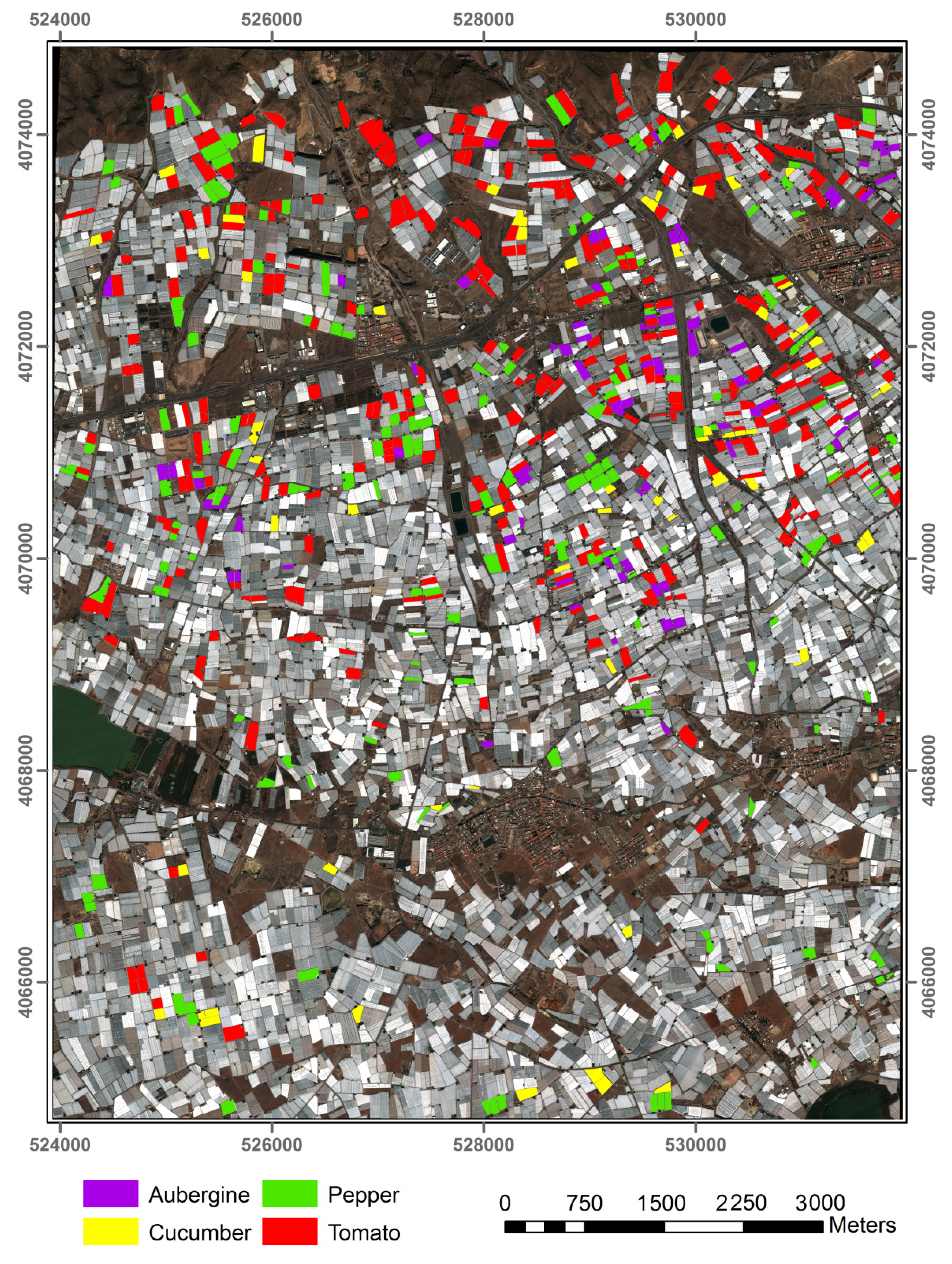
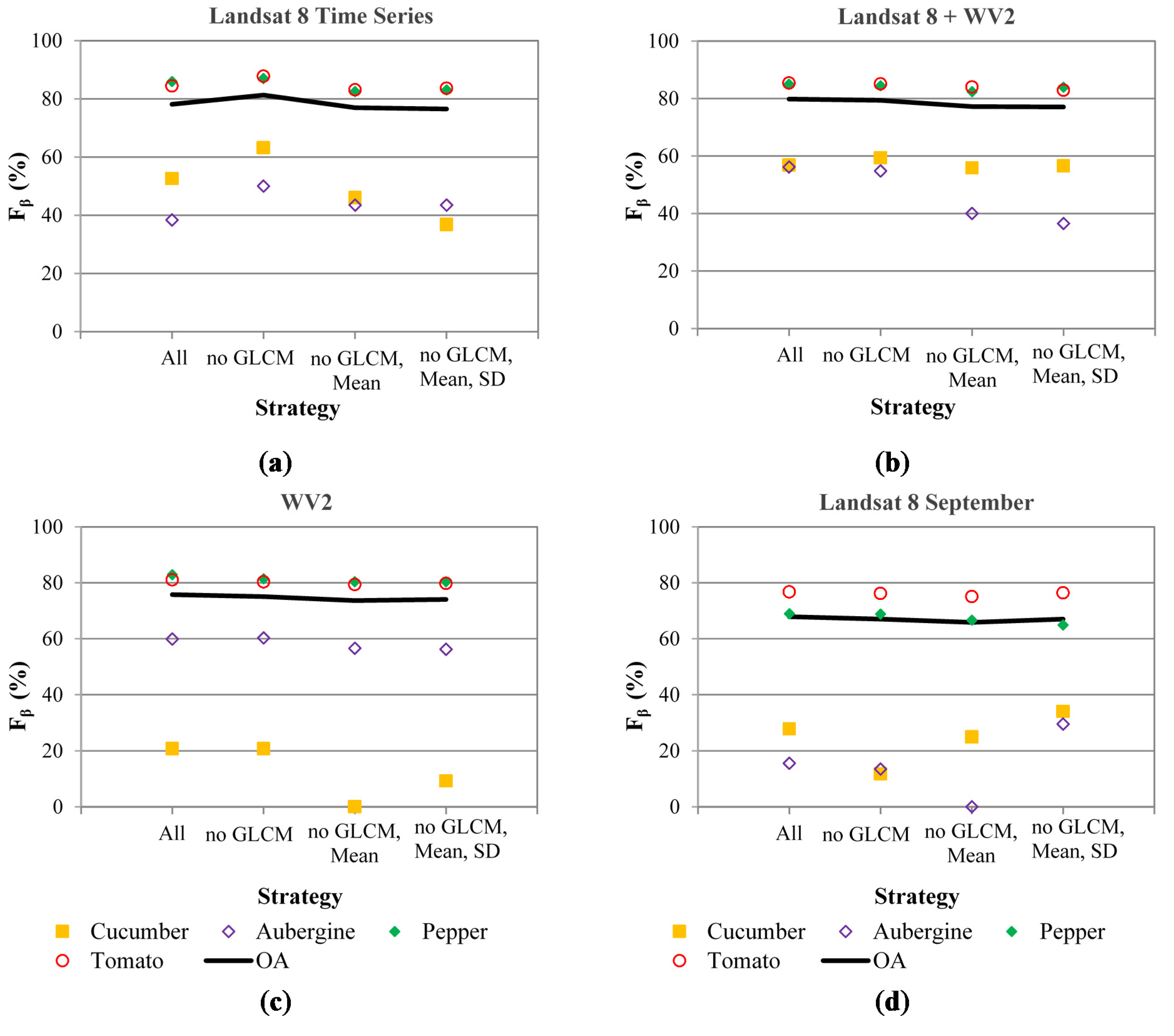
5.1. Classification Accuracy with Regard to Data Sources and Features
Three main datasets were tested in this work (i.e., only Landsat 8 time series data, only WV2 single orthoimage data and, finally, Landsat 8 time series plus WV2 single orthoimage data). In addition, a special case involving only the single Landsat 8 orthoimage taken on 12 September was conducted just to be compared with the single WV2 case taken also in September. Moreover, four strategies or groups of features were considered for each dataset: (1) all features (All); (2) all features without GLCMs (no GLCM); (3) all features without GLCMs, mean values (no GLCM, mean); and (4) all features without GLCMs, mean and standard deviation values (no GLCM, mean, SD).
Figure 4 shows the accuracy per class and OA based on the 10-fold cross-validation method for the different datasets tested. It can be noted that the best OA values were attained with the two first strategies. Furthermore, the second-order textural parameters based on GLCM added no information in order to improve the classification accuracy. Working on outdoor crops identification, Peña-Barragán
et al. [
51] reported that texture features achieved extremely poor overall accuracy as compared to spectral features. However other research found that texture attributes based on GLCM were relevant to discriminate between some crops with similar spectral responses [
24,
25]. In this sense, it is important to bear in mind that the calculation of GLCM is computationally intensive and very time consuming. Notice that, apart from GLCM descriptors, textural information is somehow included by means of SD values, which can be considered as first-order textural features. The best OA value (81.3%) was reached when using no GLCM strategy on Landsat 8 time series (
Figure 4a). When the Landsat 8 + WV2 dataset was employed, a slightly lower OA value of 79.4% was achieved with the no GLCM strategy (
Figure 4b). OA values were far worse when only a single growing season period was considered, highlighting the suitability of multi-temporal images taken along the growing season to improve under greenhouse crop discrimination. In this way, and applying the no GLCM strategy, OA values of 75.1% and 67% were achieved for WV2 and Landsat 8 September datasets, respectively (
Figure 4c,d). The better classification results found in the case of WV2 can be attributed to its much higher spatial resolution. Regarding the results from the third strategy (no GLCM, Mean) depicted in
Figure 4, it should be noted that object spectral information based on mean values could not be removed without causing a decrease in OA close to 2%. This result strengthens the importance of applying proper atmospheric corrections on the original images.
Figure 4.
Per-class accuracy given by the corresponding Fβ index and overall accuracy (OA) using different groups of features and data sources. (a) Landsat 8 time series (eight orthoimages); (b) Landsat 8 time series plus WV2 single orthoimage; (c) WV2 single orthoimage taken on September 30; (d) Image Landsat 8 taken on September 12.
The OA values of around 80% achieved in this work are rather promising as compared to those reported by other authors working with a similar methodology, but on outdoor crops. For instance, Peña-Barragán
et al. [
24] reached an OA of 79% applying the DT classifier for detecting 13 major crops cultivated in the agricultural area of Yolo County, California, USA. This classification accuracy rose up to 88% by using support vector machine (SVM) or multilayer perceptron (MLP) neural network classifiers [
51]. In another study, twelve outdoor crops and two non-vegetative land use classes were classified with 80.7% OA at cadastral parcel levels through multi-temporal remote sensing images [
48]. Furthermore, working on mapping outdoor crops (classes corn, soybean and others), an OA of 88% was reported by Zhong
et al. [
2]. Finally, Vieira
et al. [
25] applied the DT classifier to Landsat time series in a binary classification approach between sugarcane and other crops, assessing an OA of 94%.
Regarding the accuracy per class,
Figure 4 shows that tomato and pepper crops were fairly well identified for all datasets. Again, and always using the no GLCM strategy, the best
Fβ values for tomato (87.7%) and pepper (87%) were attained for the Landsat 8 time series dataset (
Figure 4a). With the same strategy, the
Fβ measure reached values of 85.1% and 84.5% for tomato and pepper, respectively, when using the Landsat 8 time series plus WV2 dataset. It is important to underline that
Fβ values for tomato and pepper crops were significantly worse for the datasets where only a single image of WV2 (80.3% tomato and 81.5% pepper) or Landsat 8 September (76.2% tomato and 68.8% pepper) were employed. On the other hand, the other two crops presented much poorer classification accuracies. The best
Fβ value for aubergine identification (60.3%) was achieved using the WV2 dataset with no GLCM strategy. Moreover, an accuracy of 63.2% in terms of
Fβ was reached in the case of cucumber for the Landsat 8 time series dataset and, again, through the no GLCM strategy. Working on 13 outdoor crops, Peña-Barragán
et al. [
24] reported
Fβ values ranging from 94% for rice to 66.7% for rye, achieving an accuracy of 80% in the case of tomato.
More detailed information about the accuracy per class is presented in
Table 5, showing the corresponding confusion matrix for the Landsat 8 time series dataset and no GLCM strategy. It can be noted that a large number of under-greenhouse aubergine crops are misclassified as tomato. In fact, aubergine and tomato crops have a similar transplant date in Almería, usually in August (
Table 1 and
Table 2). Both crops are quite heat tolerant, and in the study area, greenhouse coverings only need a slight white paint layer to protect the crops during the transplant stage. The white paint is usually washed in September or October. Regarding cucumber crops, they have very variable transplant dates, ranging from August to October (
Table 2). For early transplanted cucumber crops, the white paint is more intense to protect the small plants during their first stage. A very slight white paint is usually applied when the cucumber crops are planted in early to mid-September and even not necessary when the cucumber plants are planted very late. Furthermore, in the study area and regarding cucumber crops, it is common to rely on a double-roof in the greenhouse, which reduces radiation losses. All of these actions cause a highly variable spectral signature on the shape of the time series profile recorded from greenhouse coverings. Finally, pepper crops are mainly planted during July and August. This is a crop that needs a significant quantity of white paint to enhance the growth of the plant, as well as to protect the transplant stage. Without a doubt, this is the most unique characteristic for the autumn pepper crop in the “Poniente” region of Almería. The pepper crops are mainly misclassified as tomato or cucumber (
Table 5).
Table 5.
Confusion matrix for Landsat 8 time series dataset and no GLCM strategy. PA, producer’s accuracy.
Table 5.
Confusion matrix for Landsat 8 time series dataset and no GLCM strategy. PA, producer’s accuracy.
| Classified Data | Reference Data |
|---|
| Aubergine | Cucumber | Pepper | Tomato | ∑ | UA (%) |
|---|
| Aubergine | 36 | 7 | 5 | 32 | 80 | 45.0 |
| Cucumber | 10 | 42 | 1 | 9 | 62 | 67.7 |
| Pepper | 3 | 12 | 157 | 20 | 192 | 81.8 |
| Tomato | 15 | 10 | 6 | 329 | 360 | 91.4 |
| ∑ | 64 | 71 | 169 | 390 | 694 | |
| PA (%) | 56.3 | 59.2 | 92.9 | 84.4 | | |
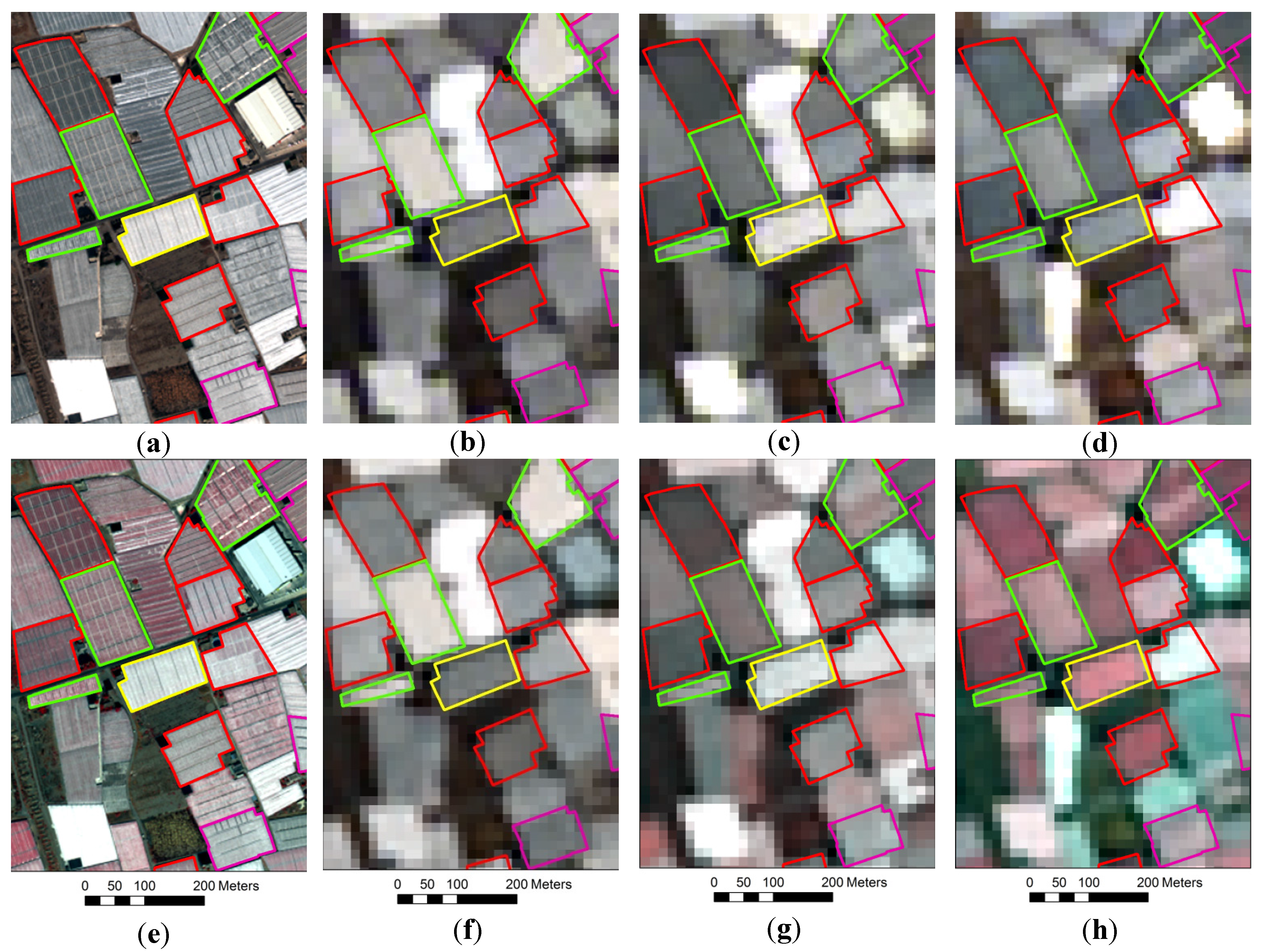
Figure 5.
WV2 MS and multi-temporal Landsat 8 pan-sharpened orthoimages showing the evolution of some reference greenhouses. (a) WV2 true color composite (RGB) 30 September; (b) Landsat 8 RGB 11 August; (c) Landsat 8 RGB 12 September; (d) Landsat 8 RGB 15 November; (e) WV2 false color composite (NIR R G) 30 September; (f) Landsat 8 false color 11 August; (g) Landsat 8 false color 12 September; (h) Landsat 8 false color 15 November. Reference objects in red, green, purple and yellow represent tomato, pepper, aubergine and cucumber crops, respectively.
In
Figure 5 is depicted the evolution of the time series profile. The cucumber greenhouse located in the center, planted on 27 August 2013, appears without white paint on 11 August (
Figures 5b,f). It seems to be whitewashed in
Figure 5a,c,e,g (30 and 12 September, respectively), and finally, this greenhouse covering is shown without any trace of paint in November (
Figure 5d,h). Moreover, November (
Figure 5h) turns out to be the month when most of the greenhouses allow one to visually perceive (false color images) the presence of crops through an increase in the NIR reflectance. This is not the case of the greenhouse located just on the right of the aforementioned cucumber one. In fact, it is a tomato crop that was whitewashed in September, and it had not yet been washed in November (
Figure 5h).
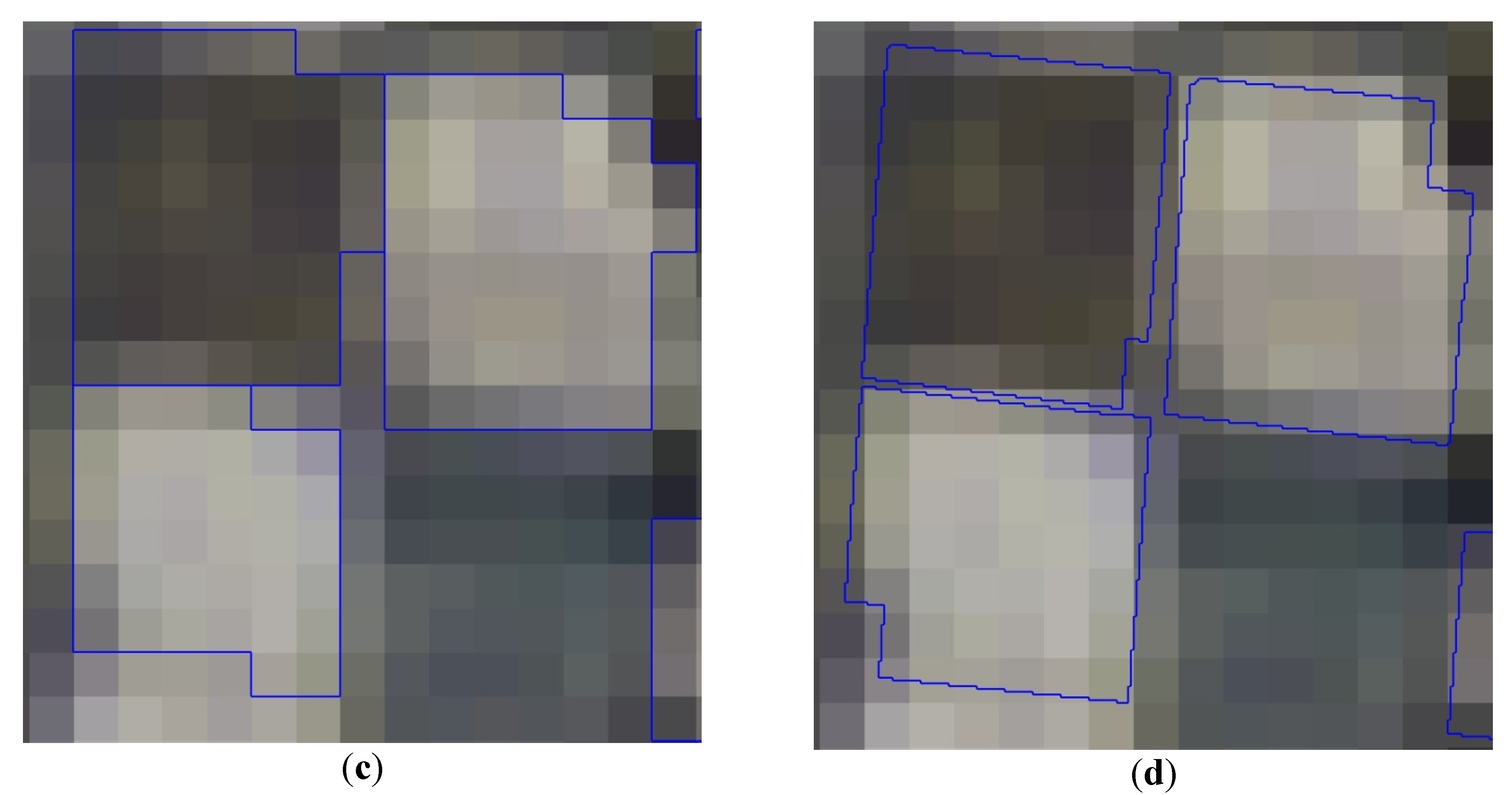
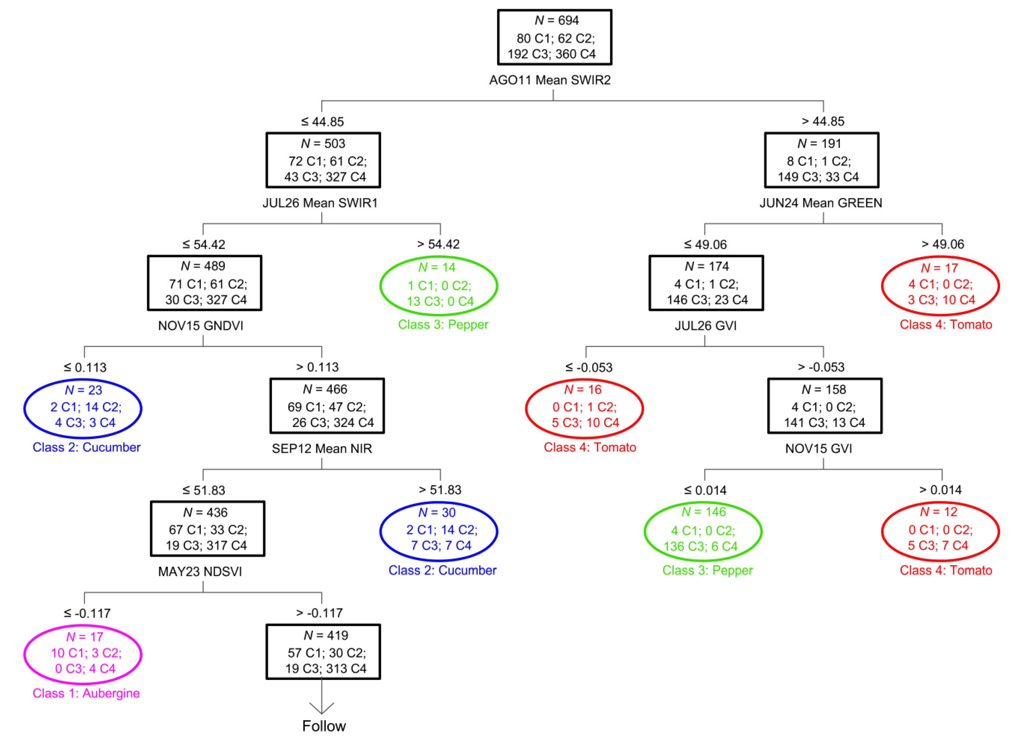
The capacity of the DT approach was used to select the object-based features and their cutting thresholds that best fit to every type of under-greenhouse crop. In view of the complexity of the computed DT, presenting up to 34 terminal nodes for the case shown in
Table 5 (Landsat 8 time series dataset and no GLCM strategy), just the first divisions of that DT (only nine terminal nodes) are presented (
Figure 6). At the bottom and outside of each black box in
Figure 6 appears the object-based feature that is causing the next split in the decision tree. Below, the readers can see the figure that represents the cutting threshold for the split. Oval nodes are terminal nodes belonging to a particular class. Thereby, the OA value attained with the pruned DT shown in
Figure 6 was 75.9%, considering the last box (
N = 419) as the Class 4 (Tomato) terminal node. It is worth noting that the object-based feature located at the top of the tree was the mean value of SWIR2 for the Landsat 8 pan-sharpened orthoimage taken on 11 August (AGO11 Mean SWIR2). SWIR2 reflectance values higher than 44.85% (right branch of the tree) were mainly associated with greenhouses that received an important dose of white paint in August, so pointing to pepper crops. In fact, 149 out of the 191 selected greenhouses with higher SWIR2 turned out to be pepper crops. The remaining high SWIR2 objects in August were identified as tomato (33 greenhouses belonging to Class 4), aubergine (eight greenhouses for Class 1) and cucumber (one greenhouse belonging to Class 2). The next steps in that branch of the DT were addressed to separate these tomato greenhouses. In this way, features, such as the mean value for the green band reflectance on 24 June, the Green Vegetation Index (GVI) on 26 July and GVI in November, were chosen to carry out this task. At the end of June, pepper greenhouses were being prepared to receive the plants, so they were usually bare and presented a lower value for the green band reflectance. Regarding GVI values for the pepper crops, they were often higher at the end of July and lower in November as compared to other crops in the study area. On the left branch of the DT (
Figure 6) we observe most of the aubergine (72), cucumber (61) and tomato (327) crops, which received low doses of white paint (SWIR2 reflectance ≤ 44.85%), but it also contained 43 greenhouses of Class 3 (Pepper). The SWIR1 mean value on 26 July was used to extract these pepper crops with a high dose of white paint when transplanted early. The rest of the object-based features used in this branch (
i.e., GNDVI in November, mean NIR in September and Normalized Differential Senescent Vegetation Index (NDSVI) in May) were aimed at discriminating tomato, cucumber and aubergine crops. The last box in
Figure 6 still contains 419 objects classified as tomato in the DT with nine terminal nodes. The whole DT, presenting 34 terminal nodes, continues from that point using the other 23 features extracted along different periods, such as mean reflectance values (NIR, Blue, SWIR2 and SWIR1), standard deviations (SWIR2, blue, green and NIR) and VIs (NDSVI, Normalized Difference Tillage Index (NDTI), GVI and GNDVI).
In view of the above, the identification of under-greenhouse pepper crops can be carried out with high success rates, mainly based on the crop management techniques applied during the growing cycle for each agricultural region. In our test field, an OA of 92.7% and a kappa coefficient of 0.81 were achieved considering only two classes (pepper and others) by using Landsat 8 time series with no GLCM strategy. In addition, a very simple DT (similar to the top part of
Figure 6) with only six terminal nodes and only five features (
i.e., AGO11 mean SWIR2, JUL26 mean SWIR1, JUN24 mean GREEN, SEP12 SD BLUE and JUL26 GVI) were required for the achievement of the aforementioned results.
Figure 6.
Decision tree computed for the Landsat 8 time series dataset and no GLCM strategy. Only nine out of 34 terminal nodes are shown. N is the number of objects in each node, Class 1 (C1) = aubergine, C2 = cucumber, C3 = pepper, C4 = tomato. AGO11, 11 August; JUL26, 26 July; JUN24, 24 June; NOV15, 15 November; SEP12, 12 September.


 ,
, 


