On Attribute Thresholding and Data Mapping Functions in a Supervised Connected Component Segmentation Framework

Abstract

Search-centric, sample supervised image segmentation has been demonstrated as a viable general approach applicable within the context of remote sensing image analysis. Such an approach casts the controlling parameters of image processing—generating segments—as a multidimensional search problem resolvable via efficient search methods. In this work, this general approach is analyzed in the context of connected component segmentation. A specific formulation of connected component labeling, based on quasi-flat zones, allows for the addition of arbitrary segment attributes to contribute to the nature of the output. This is in addition to core tunable parameters controlling the basic nature of connected components. Additional tunable constituents may also be introduced into such a framework, allowing flexibility in the definition of connected component connectivity, either directly via defining connectivity differently or via additional processes such as data mapping functions. The relative merits of these two additional constituents, namely the addition of tunable attributes and data mapping functions, are contrasted in a general remote sensing image analysis setting. Interestingly, tunable attributes in such a context, conjectured to be safely useful in general settings, were found detrimental under cross-validated conditions. This is in addition to this constituent’s requiring substantially greater computing time. Casting connectivity definitions as a searchable component, here via the utilization of data mapping functions, proved more beneficial and robust in this context. The results suggest that further investigations into such a general framework could benefit more from focusing on the aspects of data mapping and modifiable connectivity as opposed to the utility of thresholding various geometric and spectral attributes.

1. Introduction

Research into operational remote sensing image analysis methodologies continues to enjoy attention in response to real-world requirements within the private and public sectors. This is evident in the variety of journals, conferences, and workshops within the context of remote sensing methodology, with a concomitant increase in niche interdisciplinary sub-disciplines. Two examples, dealing mainly with optical data, are Geographic Object-Based Image Analysis (GEOBIA) [1] and mathematical imaging within remote sensing [2]. This contribution falls within the context of these two sub-disciplines.

A new variant of sample supervised segment generation is analyzed, recently presented as a conference contribution [3]. Sample supervised segment generation denotes a general search-centric methodological framework for generating quality image segments based on the provision of a selection of exemplar segments [4,5,6,7]. Segments generated via such an approach may be used in further processes to progress to a final information product. A connected component (quasi-flat zone) segmentation algorithm, specifically an attribute-enhanced variant of Constrained Connectivity (CC) [8,9,10,11], is embedded into such a sample supervised segment generation framework. The modular and extendable nature of the segmentation algorithm allows for the definition of arbitrary attribute criteria to assist in shaping the nature of the generated segments. Such tunable attribute criteria are cast as an additional parameter constituent within the sample supervised segment generation framework. Additionally, data transformation or mapping functions [6] may be added as a constituent in such a framework. Utilizing mapping functions falls within the context of defining connected components more elaborately, also considered for connected component segmentation algorithms via additional processing (pre-filtering/post-filtering) [12,13], via analyzing scene-wide statistics [14,15], and via the notion of hyperconnections [16,17,18]. Adding mapping functions into such a framework results in three distinct, interdependent parameter constituents that need consideration.

The contribution of this work is two-fold. Firstly, the feasibility of the proposed framework is analyzed to demonstrate that it constitutes a valid optimization problem, having interacting constituents and being searchable via metaheuristics. The presented method may be cast as four separate variants, using various constituent combinations. Secondly and primarily, the relative merits of the two added constituents are contrasted, namely that of additional mapping functions and that of tunable attribute criteria. It is demonstrated in a selection of remote sensing image analysis problems, under various metric conditions and also under cross-validated conditions, that utilizing geometric and attribute criteria to shape the nature of the generated segments may be detrimental. This suggests more careful consideration in the utilization of attributes in the context of such a framework.

This paper is structured as follows. Section 2 presents an overview and review of background principles related to the segmentation approach used, as well as some aspects of a sample supervised segment generation framework. In Section 3, the investigated method and its variants are detailed. The data used are described in Section 4. In Section 5, the method is experimentally evaluated and its variants are contrasted. Concluding comments and prospects for future work are given in Section 6.

2. Background and Related Work

2.1. Graph-Based Connected Component Segmentation

Graph-based connected component segmentation defines a family of image-processing methods stemming from work within the broader context of mathematical morphology. See [19] for a general overview of mathematical morphology and [20] for an overview of segmentation concepts and approaches. Developments and applications within remote sensing mirror the advancements of basic research within mathematical morphology. Classic mathematical morphology tools (erosion, dilation, and reconstruction filtering) [19] found successful applications within remote sensing, e.g., [21,22].

A major development in the proliferation of applications of mathematical morphology tools in remote sensing is the notion of a flat zone. A flat zone defines a specific level in a hierarchical image partitioning based on grey-level intensities [20,23,24]. Various successful methods and applications have been presented based on this notion, e.g., [2,25,26,27,28]. This development was elaborated upon with the notion of a quasi-flat zone, which relaxes the restrictive definition of a flat zone by introducing a certain level of dissimilarity tolerance between pixels (parameter controlled) [8,9,20,29]. Quasi-flat zones form the basis of flexible segmentation algorithms, suited to remote sensing image analysis problems. Resultant segmentation algorithms have attractive properties, including ease of extensibility and inherent modularity [16,29], computational and memory efficiency [9,30,31] (especially in hierarchical formulations), uniqueness (same segmentation on repeated runs, some formulations [8]), and mathematically rigorous formulations. Efficient data structures and computational efficiencies are major considerations in such approaches. Comparative and practical analyses with other commonly used segmentation algorithms within remote sensing are needed, e.g., [32].

2.2. Constrained Connectivity

Constrained Connectivity (CC) is an image partitioning or simplification (segmentation) method based on the identification of quasi-flat zone connected components [8,10,11,13,29]. Spectral difference or grey-level difference is defined as a connectivity relation, denoted by α (alpha) and called the local range (parameter). Other constraints may be introduced. This notion was originally developed to address the chaining effect of the single linkage clustering method [8]. Quasi-flat zone approaches may be considered an alternative or extension of the mathematical morphology approaches applied in remote sensingthat considers image local extrema in processing, e.g., [23,33,34]. The algorithm is hierarchical, with a fully calculated hierarchy known as an alpha tree. Within an alpha tree, all constraints (parameter combinations) are calculated and stored in a tree data structure [9,31], with connected components efficiently computed via Tarjan’s union-find algorithm [9,31] (or others).

CC may be defined as the partitioning of an image into α-connected (alpha) components. Two pixels are considered connected (α-connected) if there exists a path between them such that the grey-level difference of successive pixels in this path does not exceed a given value (α). The connected component (segment) of a given pixel p and other pixels q for a given α may be denoted as follows:

$$\alpha -CC\left(p\right)=\left\{p\right\}{{\displaystyle \cup }}^{\text{}}\text{{}q\text{|} a path S=\left(p=p_1,\dots ,p_n=q\right), n>1, such that D\left(p_i,p_{i+1}\right)\le \alpha for all 1 \le i <n\}$$

(1)

D denotes a range function that calculates the difference between the spectral values of two given connected pixels. Note that successive segmentations of $\text{α}$-CC are hierarchical (increasing α values) and that a unique partition (identical over various runs) is generated. Various approaches [8,31] may be followed for computing an $\text{α}$-CC segmentation efficiently, with a priority queue approach followed here [8].

A useful additional parameter, namely the global range criterion (w), may also be introduced. w constrains the creation of connected components by limiting the maximum spectral difference between any two pixels in a connected component. Additional constraining attributes (increasing/non-increasing) (“Attr”) may also be further introduced via predicates evaluating the potential connected components. The connected component of a pixel may then be described as:

$$\left(\alpha ,w\right)-CC\left(p\right)=\left\{p\right\}{{\displaystyle \cup }}^{\text{}}\text{{}q\text{|} a path S=\left(p=p_1,\dots ,p_n=q\right), n>1, such that D\left(p_i,p_{i+1}\right)\le \alpha for all 1 \le i <n and Max\left(S\right)-Min(S)\le w\}$$

(2)

with a further predicate (P) able to restrict the growth defined for a given connected component (X) as:

$$P\left(\left(\alpha ,w\right)-CC\left(p\right)\right)= true if Attr\left(X\right)\le t, false otherwise$$

(3)

where t denotes a threshold value for a given attribute (e.g., segment area) and Attr a function calculating the value of the attribute. For example, during the computation of connected components, if a given potential connected component (e.g., X) satisfies the local and global range criteria $\left(\text{α},\text{w}\right)$, but the calculated area attribute of the potential connected component exceeds a given threshold value (t), it is not substantiated. If the calculated area attribute is below the given threshold value, the connected component is substantiated (a visual example of constraining attributes is given in Section 3).

Max(S) and Min(S) return the maximum and minimum spectral values within path S, respectively. Various approaches exist to handle multichannel imagery [8,35,36]. Here a constraint is simply triggered for the entire given image (all bands) if any of the composite bands trigger a constraint.

Figure 1 illustrates an abstract image, with pixel values labeled with their intensity values, as well as shaded for easier visualization (lower value = brighter pixel). Bold lines delineate connected component borders. Figure 1a shows an image segmented ($\alpha$w-CC) with (0,0)-CC, (1,1)-CC (Figure 1b), (1,2)-CC (Figure 1c), and (2,3)-CC (Figure 1d). Dotted lines denote an absence of a path between two pixels for the given constraints.

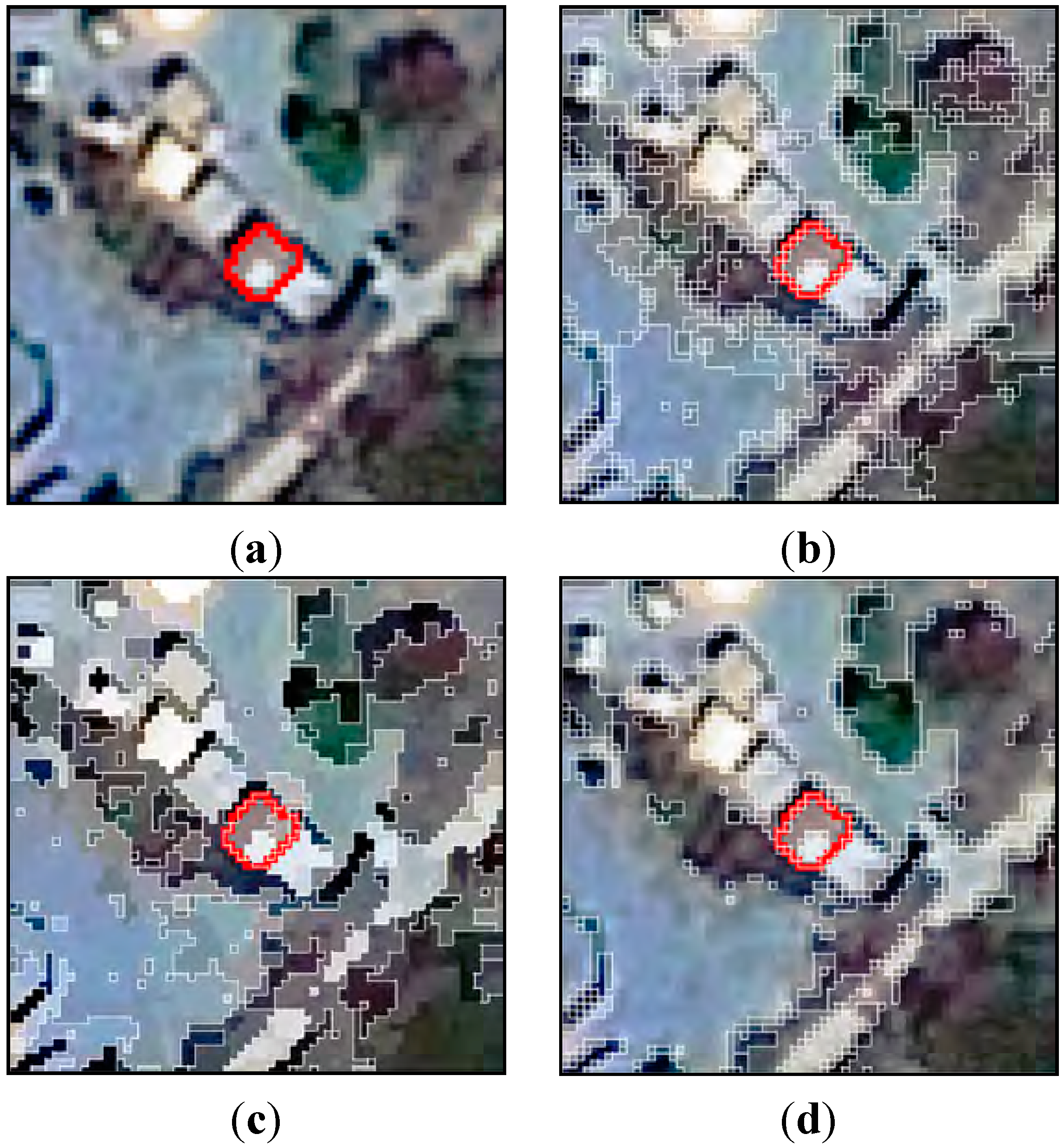
Figure 2 shows segmentation results using $\text{α}$w-CC on a subset of a real image (arbitrary) to highlight general characteristics. Transition regions [10] are characterized by multiple single pixel connected components in areas where the transition between homogeneous areas spans several pixels. Some approaches may be applied to diminish this effect [10,12] (Figure 2c—Iterative area filtering), not considered here owing to experimental anomalies observed with such additional processing. Post-processing may simply be applied to remove single pixels (among others). A structure is delineated with a red polyline (example element of interest) (a), with segmentation results shown using (25,75)-CC (b), a pre-processed [10] image segmented with (25,75)-CC (c) to minimize the effect of transition regions and (50,200)-CC (d).

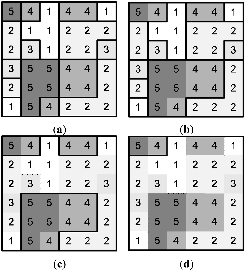
Figure 1. An abstract image, segmented with the $\alpha$w-CC method illustrating its general characteristics, with (0,0)-CC shown in (a), (1,1)-CC in (b), (1,2)-CC in (c), and (2,3)-CC in (d).

Figure 1. An abstract image, segmented with the $\alpha$w-CC method illustrating its general characteristics, with (0,0)-CC shown in (a), (1,1)-CC in (b), (1,2)-CC in (c), and (2,3)-CC in (d).

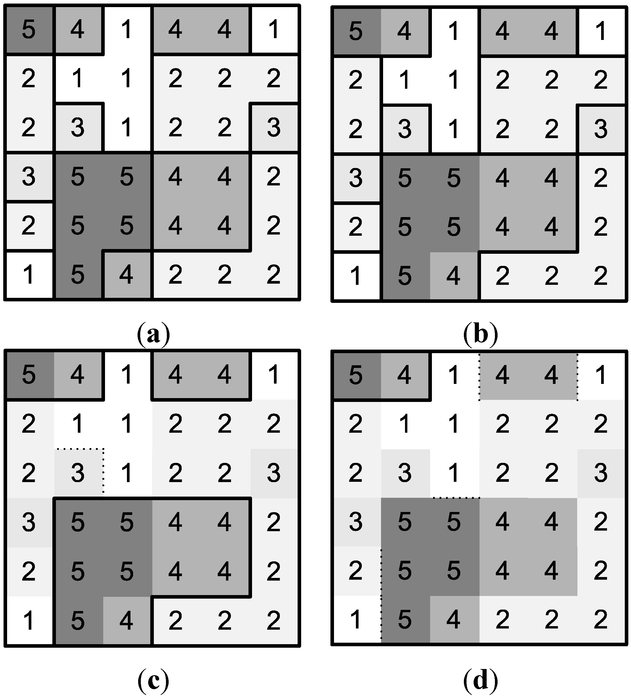
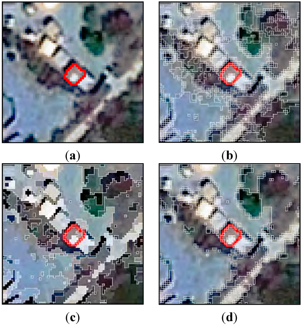
Figure 2. An image subset (a) segmented with ($\alpha$w-CC) to show its common characteristics on real imagery, with the local and global range parameters set to 25 and 75 (b), 25 and 75 with a region growing filter (c), and to 50 and 200 (d), respectively. The red polyline indicates an example element a user might be interested in.

Figure 2. An image subset (a) segmented with ($\alpha$w-CC) to show its common characteristics on real imagery, with the local and global range parameters set to 25 and 75 (b), 25 and 75 with a region growing filter (c), and to 50 and 200 (d), respectively. The red polyline indicates an example element a user might be interested in.

2.3. Metaheuristics

Metaheuristics constitutes a class of optimization algorithms (minimization or maximization) which are commonly multi-agent and stochastic in nature, and contain elements of search intensification and search diversification (see e.g., [37] for an overview). Many metaheuristic algorithm designs are inspired by naturally occurring search processes. Their main practical utility is in reducing computing costs to obtain optimal, or, more typically, near optimal results. Their application needs careful consideration in the choice of metaheuristic to be used (applicability, no free lunch theorem, search landscape characteristics), the handling of meta-parameters (meta-optimization, self-adaptation, empirical tuning, hyper-heuristics) and the nature of statistical evaluations and reporting being some examples [38,39,40,41,42]. Their utility in a certain context may be evaluated via experimentation [39], with robustness, absolute and relative results, standard deviation, required computing times, and search process characterization some of the measurable aspects. Their application in remote sensing image analysis is wide; they are employed for feature selection and generation, classification processes, and various image-processing tasks.

Here a selection [43] of classic metaheuristics and simpler search algorithms is employed and evaluated as parameter optimizers in the investigated framework. More specifically, classic variants of two well-known real-valued population-based optimizers are used, namely Differential Evolution (DE) [44] and Particle Swarm Optimization (PSO) [45]. The “DE/rand/1/bin” [44] variant of DE is used with meta-parameters empirically tuned (30 Agents, F = 0.75, CR = 0.3). Similarly, for PSO (30 Agents, Inertia Weight = 0.7, Best own weight = 1.5, Best weight = 1.5). A Hill Climber (HC) is also employed (D = 30), along with random sampling (RND).

2.4. Empirical Discrepancy Metrics

Empirical discrepancy metrics [46] constitute a family of measures used to evaluate the quality of image segmentation. They are supervised, as they need a reference or ground truth to compare generated results with produced results. Notions of geometry, overlapping area, boundary offsets, and content are commonly encoded in such metrics, either via producing a singular result or as separate results (multi-objective frameworks). Analytical or unsupervised measures may also be considered [47]. A selection of empirical discrepancy metrics is employed here, namely the Reference Weighted Jaccard (RWJ) [6], Reference Bounded Segments Booster (RBSB) [48], and the Partial and Directed Object-Level Consistency Error (PD_OCE) [6,49]. They are chiefly based on the concept of area overlap, with the ability to measure notions of over- and under-segmentation. These metrics are summarized in Table 1 ([6,48,49]) (set theory notation), with R and S denoting a reference and generated (S) segment respectively. I is an iterator running through all generated segments (S) intersecting R. Their formulations are substantially different (some more precise, some more general), allowing for a varied interpretation of results and also for creating variation in search landscape characteristics (when employed to direct a search process). The optimal result for an evaluation is zero.

Table 1. The three empirical discrepancy metrics employed to measure the quality of generated segments against the provided reference segments.

Metric	Formulation	Reference
RWJ	$1-{\displaystyle \sum _{i=1}^n}\frac{\left|R {\displaystyle \cap } S_i\right|}{\left|R {\displaystyle \cup } S_i\right|}\times \frac{\left|R {\displaystyle \cap } S_i\right|}{\left|R\right|}$	[6]
RBSB	$\frac{\left|R {\displaystyle \cup } S\right|-\left|R {\displaystyle \cap } S\right|}{\left|R\right|}$	[48]
PD_OCE	$1-{\displaystyle \sum _{i=1}^n}\frac{\left|R {\displaystyle \cap } S_i\right|}{\left|R {\displaystyle \cup } S_i\right|}\times \frac{\left|S_i\right|}{{{\displaystyle \sum }}_{j=1}^n\left|S_j\right|}$	[6,49]

Table 1. The three empirical discrepancy metrics employed to measure the quality of generated segments against the provided reference segments.

Metric	Formulation	Reference
RWJ	$1-{\displaystyle \sum _{i=1}^n}\frac{\left|R {\displaystyle \cap } S_i\right|}{\left|R {\displaystyle \cup } S_i\right|}\times \frac{\left|R {\displaystyle \cap } S_i\right|}{\left|R\right|}$	[6]
RBSB	$\frac{\left|R {\displaystyle \cup } S\right|-\left|R {\displaystyle \cap } S\right|}{\left|R\right|}$	[48]
PD_OCE	$1-{\displaystyle \sum _{i=1}^n}\frac{\left|R {\displaystyle \cap } S_i\right|}{\left|R {\displaystyle \cup } S_i\right|}\times \frac{\left|S_i\right|}{{{\displaystyle \sum }}_{j=1}^n\left|S_j\right|}$	[6,49]

2.5. Sample Supervised Segment Generation

Sample supervised segment generation comprises a general image processing approach where an image segmentation task is cast as a search or optimization problem. A segmentation algorithm is defined, with its controlling aspects cast as variables or parameters forming a multidimensional search problem. Such an approach was initially proposed to simply tune the free parameters of a given segmentation algorithm for a given image analysis task [4]. Research into this general approach has been presented in various image analysis disciplines e.g., [4,7,50], including remote sensing [5,6,51]. Generally an appropriate level of a hierarchical segmentation algorithm is sought for a given image element type (e.g., specific buildings). In general, metaheuristics are employed as optimizers and empirical discrepancy metrics to drive the search process. Alternatively said, empirical discrepancy metrics may define the search landscape. Note that sample supervised segment generation is a specific implementation of the more general notion of image analysis via efficient search. See [52] for a primer. The method presented in Section 3 follows this general approach of sample supervised segment generation, where more detail may be found.

Various aspects of such an approach have been examined, including the applicability of various search methods e.g., [6,51], metric behavior [53,54] and the performance of domain-specific segmentation algorithms in this context [6,50]. Generalizability to unseen data, sampling requirements, method extensions, and method integration are open topics [6,54,55]. Note that parameters may also define construction processes of lower-level building blocks for image analysis, with mathematical morphology and genetic programming well suited to such designs [56,57].

3. Method

3.1. Method Details

A variant of sample supervised segment generation is presented [3] (conference paper), incorporating mapping functions for data adaptation and additional attributes for constraining segment growth. Figure 3 illustrates the architecture of the method, which is based on the general architecture of sample supervised segment generation [4]. The main distinguishing aspect of this variant is the three interacting parameter constituents handled by the given optimizer.

Initially a selection (5–50) of samples or reference segments is provided for the method, obtainable by various means (manual, semi-automated, or automated). A pre-processing phase conducted exclusively to save computing costs extracts image subsets centered over the reference segments. This may impact results in scenarios with non-unique segmentation algorithms. CC as used here generates unique results. The image subsets and accompanying reference segments are given as input to the optimization loop (see Figure 3).

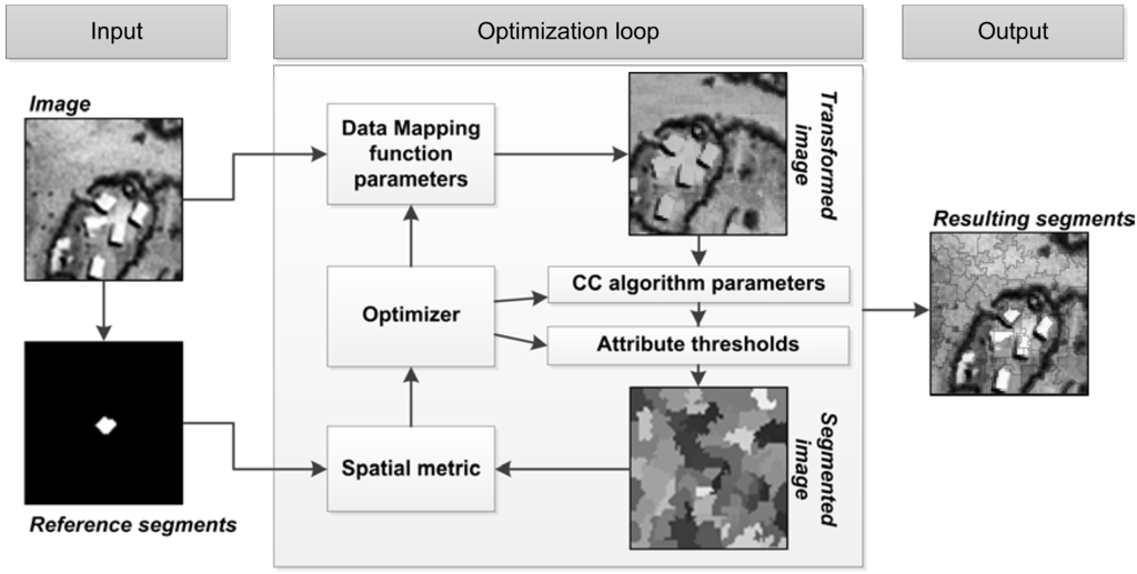
Figure 3. The architecture of the sample supervised segment generation method incorporating data mapping functions and attribute thresholding [3]. IEEE^© 2013. Reprinted, with permission, from [3].

Figure 3. The architecture of the sample supervised segment generation method incorporating data mapping functions and attribute thresholding [3]. IEEE^© 2013. Reprinted, with permission, from [3].

During the optimization loop phase, an optimizer (e.g., DE) traverses a parameter set over a certain number of iterations, which may control various image-processing functions on the image subsets. Three constituent parameter sets are defined in this method. Firstly, the controlling parameters of a given data mapping function transform or map the image subsets to a new domain. A few mapping functions are investigated with this method, detailed in Section 3.2. The transformed image subsets are subjected to the CC segmentation algorithm, with the optimizer providing the values for the local and global range parameters. This two-dimensional parameter set is the second constituent. The third constituent is a selection of segment spectral and geometric attributes, with the generated values defining attribute thresholds preventing segment growth within the attribute-enhanced CC framework. The image subsets are thus transformed and segmented, with the three-parameter constituents controlling the characteristics of the generated segments.

The generated segments are evaluated (averaged) against the provided reference segments via a given empirical discrepancy metric. The RWJ, PD_OCE, and RBSB metrics are used here. The metric score is given to the optimizer as feedback of the performance of the given parameter set (all three constituents). The optimizer uses the information on quality to direct its search process for the next iteration of the optimization loop. Various termination criteria are possible for the optimization loop; here it is simply terminated after a certain number of iterations.

Finally after the optimization loop terminates, the best performing parameter set is given as output. The entire image may subsequently be segmented with the same image processing as employed in the optimization loop, with the image processing operators set with the output parameter set. Note that data mapping is conducted for segment generation and the byproduct is not used in further image processing. Also, the search process is used only during the training phase.

Note that there exists an optimal achievable result, within all the parameter value combinations. This result may not be perfect, i.e., not match the provided reference segments exactly, but is as good as it can get. In practice an exact match is highly unlikely. Also note that a search method may fail in finding the optimal achievable result. Multiple optimal achievable results are also possible, e.g., multiple parameter sets delivering the same optimal achievable metric score.

The three parameter constituents of the method are evaluated for their relative usefulness in a general setting. The presented method may function in four distinct ways. Firstly, the method may simply optimize the two parameters of CC, without any extra data mapping of attribute thresholding processes. This variant is simply called CC. Secondly, additional constraining attributes may be introduced, with this variant called CC + Attr (Attributes). Alternatively, CC may function with an additional mapping function, called CC + Map (Mapping function). As depicted in Figure 3, the full method entails tuning all three constituents, called CC + Attr + Map. Figure 4 illustrates an example of an 11-dimensional parameter set traversed by an optimizer in the full formulation of the method (CC + Attr + Map). Constituents are detailed in the next sections.

Figure 4. An example of an 11-dimensional parameter set traversed by the CC + Map + Attr full method variant. Example parameters within each constituent are written vertically.

Figure 4. An example of an 11-dimensional parameter set traversed by the CC + Map + Attr full method variant. Example parameters within each constituent are written vertically.

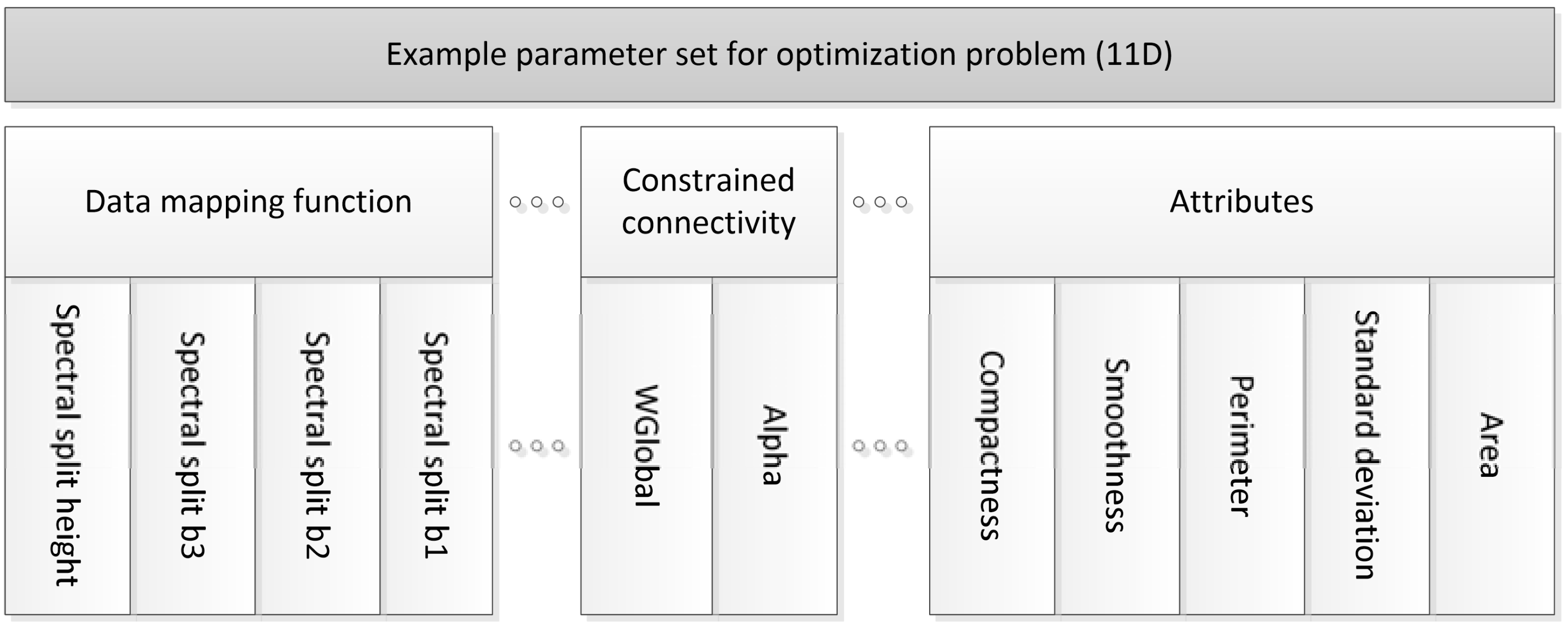
In the situation of discrete parameter quantization (byte and short in this implementation), Figure 4 illustrates an optimization problem with more than $3\times {10}^{23}$ unique parameter combinations. The nature of the image processing (which these parameters control) dictates the difficulty of the search problem. An efficient search method may only search a fraction of such a space to obtain an optimal or near optimal result. This is strongly dependent on the “searchability” of the resultant search surface [4]. The validity of the proposed method as a valid optimization problem is also investigated, with a selection of optimizers experimentally evaluated. Details of the mapping functions used and their attribute constituents are briefly given.

3.2. Mapping Functions

In the generic formulation of CC, basic dissimilarity is defined by the spectral difference between two pixels. Alternative definitions of connectivity may be considered as detailed in Section 2.2. In this work an indirect approach is followed, where spectral dissimilarity is changed externally via a data mapping function. Adding mapping functions shows promise for increasing the optimal achievable segmentation quality in similar frameworks in the context of remote sensing image analysis [6]. Some works have been proposed to reduce the influence of gradient zones based on external processing [8,13] in the context of CC. Three mapping functions are tested [6], briefly described below. Figure 5 illustrates example results by running these functions. In this work three image bands (eight-bit quantization) are assumed.

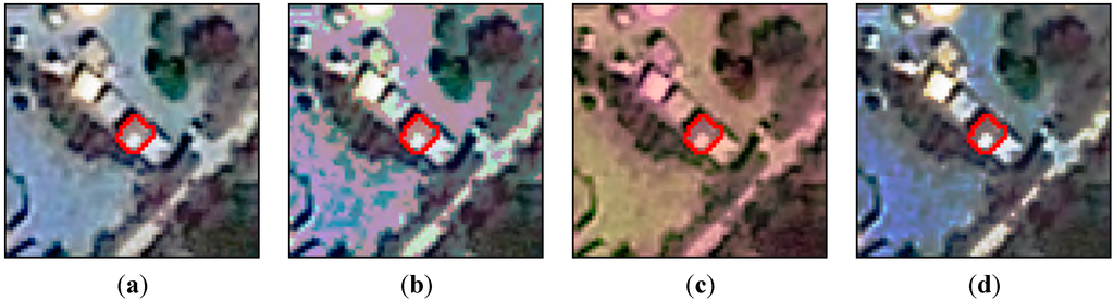
Figure 5. Example output of the three used mapping functions on an arbitrary test image (a). Parameters were assigned random values. The red polyline denotes an example element of interest; (b) shows output of the SS function (note the creation of sharp gradients);(c) shows output from the transformation matrix, while (d) shows the output from the GT function. Note the non-linear stretch of the output from the GT function.

Figure 5. Example output of the three used mapping functions on an arbitrary test image (a). Parameters were assigned random values. The red polyline denotes an example element of interest; (b) shows output of the SS function (note the creation of sharp gradients);(c) shows output from the transformation matrix, while (d) shows the output from the GT function. Note the non-linear stretch of the output from the GT function.

3.2.1. Spectral Split

Spectral Split (SS) [6] is a simplistic function able to create artificial edges in gradient zones, based on the tuning of two parameters. It is given by:

$$f\left(x\right)=x-\left(x-p\right)+sign\left(x-p\right)\times h, if abs\left(x-p\right)\le h, else f\left(x\right)=x$$

(4)

where p defines a position in the spectral domain (band specific) and h defines the magnitude of spectral change around the given spectral position (p); x remains unchanged if not falling within the required bounds (h). The function is useful in scenarios where the boundaries of elements of interest are not distinct or span multiple pixels. Sign extracts the sign of the number, with zero given a positive sign.

3.2.2. Transformation Matrix

A transformation matrix (LIN) with three image bands is used as a mapping function. Considering three input bands, nine parameters (a–i) define the transformation matrix. A pixel (n1–n3/b1–b3) is defined by the point matrix:

$$\left[\begin{array}{c}n1\\ n2\\ n3\end{array}\right]=\left[\begin{array}{c}a b c\\ d e f\\ g h i\end{array}\right]\left[\begin{array}{c}b1\\ b2\\ b3\end{array}\right]$$

(5)

The range of the parameters is set to [−0.2, 1], allowing for the enhancement of negative band correlations if present and if found useful by a search process.

3.2.3. Genetic Transform

A function, developed as a parameterized low-level image processing method for image enhancement [58], consists of four parts conducting data stretching (parameters p1–p5) and weighs their contribution based on additional weighting parameters (parameters p6–p10). For convenience the function is called Genetic Transform (GT). It is written as:

$$f\left(x\right)=\frac{log(1+e^{p1-1} \times x)}{p1}\times p7+\frac{{(1+p2)}^x-1}{p2}\times p8+\frac{1}{1+{(\frac{(1-x)}{p3})}^{p4}}\times p9+\frac{1}{{(\frac{1}{x}+p6-1)}^{p5}}\times p10$$

(6)

As with the SS function, the GT function may assist in sharpening boundaries in image elements. In the case of GT, this is achieved via parameterized non-linear data stretching.

3.3. Attributes

Six attributes are defined for consideration as additional thresholding criteria in the presented method. Table 2 summarizes the used attributes and their given ranges. Area, variance, and perimeter are simple attributes, conjectured to add some benefit in many instances. The gray level difference histogram (CH), defined here with five bins (CH1–CH5), counts the number of instances of gray level differences in a segment falling within the given bin constraint. Here a 4-connected pixel design is considered. The bin ranges are given in Table 2. For example, if a segment contains only two pixels and the spectral difference between them is 7 (intensity difference), the second bin (CH2) will have a value of 1. The other bins (CH1, CH3, CH4, CH5) will have a value of zero.

Note the intrinsic link between the gray level difference histogram bins and the local and global range parameters of CC. Small values of the local and global range parameters may lead to empty CH bins. All attributes are computed incrementally during the execution of CC (if attributes are used).

Table 2. Implemented attributes for consideration in the context of CC segmentation, specifically in the CC + Attr and CC + Attr + Map method variants.

Attribute	Range	Description
Area	[0..500]	Segment area measured in number of pixels
Standard Deviation	[0..255]	Segment spectral standard deviation
Perimeter	[0..500]	Number of pixel edges forming the perimeter
Smoothness (SMT)	[0..30]	Perimeter/sqrt(area)
Compactness (CMP)	[0..30]	Perimeter/bounding box edge length
Gray level difference Histogram, five bins (CH1–5)	[0..500] Bins: CH1:[0..5], CH2:(5..10], CH3:(10..15], CH4:(15..20], CH5:(20..255]	Number of edge weights falling within specified bins. Five bins are defined.

Table 2. Implemented attributes for consideration in the context of CC segmentation, specifically in the CC + Attr and CC + Attr + Map method variants.

Attribute	Range	Description
Area	[0..500]	Segment area measured in number of pixels
Standard Deviation	[0..255]	Segment spectral standard deviation
Perimeter	[0..500]	Number of pixel edges forming the perimeter
Smoothness (SMT)	[0..30]	Perimeter/sqrt(area)
Compactness (CMP)	[0..30]	Perimeter/bounding box edge length
Gray level difference Histogram, five bins (CH1–5)	[0..500] Bins: CH1:[0..5], CH2:(5..10], CH3:(10..15], CH4:(15..20], CH5:(20..255]	Number of edge weights falling within specified bins. Five bins are defined.

Figure 6 illustrates the same image subset as shown in Figure 2, with the local range parameter set to 50 and the global range parameter to 200, but with additional constraining attributes added for illustration. Specifically, Figure 6a shows the addition of the area attribute set to 800 in this instance. Compare with Figure 2d, where the local and global range parameters are the same. Figure 6b shows the addition of the CH1 bin, set to 300. Intuitively the impact of the constraints may be interpreted as the largest segments possible (hierarchical) under a local range of 50 (or lower), still satisfying a global range of 200 in addition to an area criterion of 800 (Figure 6a) or a CH1 criterion of 300 in the case of Figure 6b.

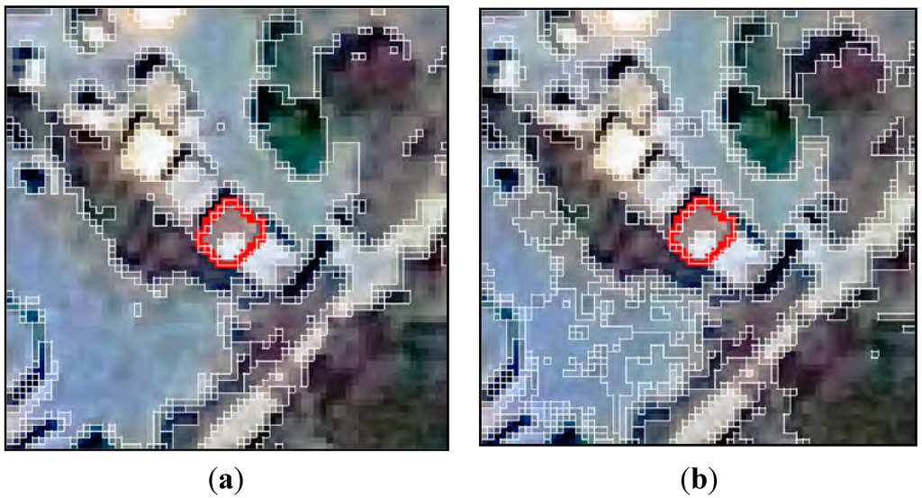
Figure 6. An image subset segmented with the local range parameter set to 50 and the global range parameter set to 200. Additional constraining attributes are introduced, specifically area, with a value of 800 (a) and CH1 (b) with a value of 300.

Figure 6. An image subset segmented with the local range parameter set to 50 and the global range parameter set to 200. Additional constraining attributes are introduced, specifically area, with a value of 800 (a) and CH1 (b) with a value of 300.

4. Data

Three image analysis tasks or problems were defined for evaluating the performance of the method variants (subset of data used in [6]). The aim was to segment structure subtypes accurately. The resulting segmentation, of maximal achievable quality, may be used in further processing methodologies. For each dataset a characteristic structure type was identified and defined as the element of interest.

Figure 7 illustrates subsets of the data and enlargements over elements of interest. Site 1, titled Bokolmanyo, depicts a refugee camp with easily identifiable tents as the elements of interest. In practice this problem could be approached with a simple single-layer segmentation and classification method. Site 2 (Jowhaar) and Site 3 (Hagadera) depict more difficult image analysis problems. The Jowhaar problem entails segmenting metal-roofed structures, with variation in roof geometry and reflectance angles ensuring a more challenging problem. Similarly the Hagadera problem entails segmenting metal-roofed structures, but with much larger variations in reflectance and geometry. A range of problem difficulties is thus presented, with a comparative analysis of segment quality the focus, rather than the final segmentation accuracies.

For each problem a number of reference elements were digitized and used as input to the presented method variants. Table 3 details some metadata of the three datasets used. All imagery consists of three bands, fully preprocessed and standardized to 8-bit quantization. The number of reference segments used is also given. Two-fold cross-validation is performed in experimentation, thus a random selection of half of the reference segments is used to drive the search process. The training and testing sets are constantly changed between experimental runs. Preliminary experimentation with varying sampling sizes was conducted to find stable results under cross-validated conditions. At least 20 runs per experiment are also advocated (detailed in the next section). This coupled with two-fold cross-validation in each run ensures a measure of generalizability in results. Note that study area size is not an important consideration. Subset images are generated, centered on the provided reference segments (e.g., Figure 2, Figure 5 and Figure 6).

Figure 7. The three image analysis tasks defined for evaluating the method variants, namely, thematically correctly segmenting tents in the Bokolmanyo problem (a) and metal-roofed structures in the Jowhaar (b) and Hagadera (c) problems.

Figure 7. The three image analysis tasks defined for evaluating the method variants, namely, thematically correctly segmenting tents in the Bokolmanyo problem (a) and metal-roofed structures in the Jowhaar (b) and Hagadera (c) problems.

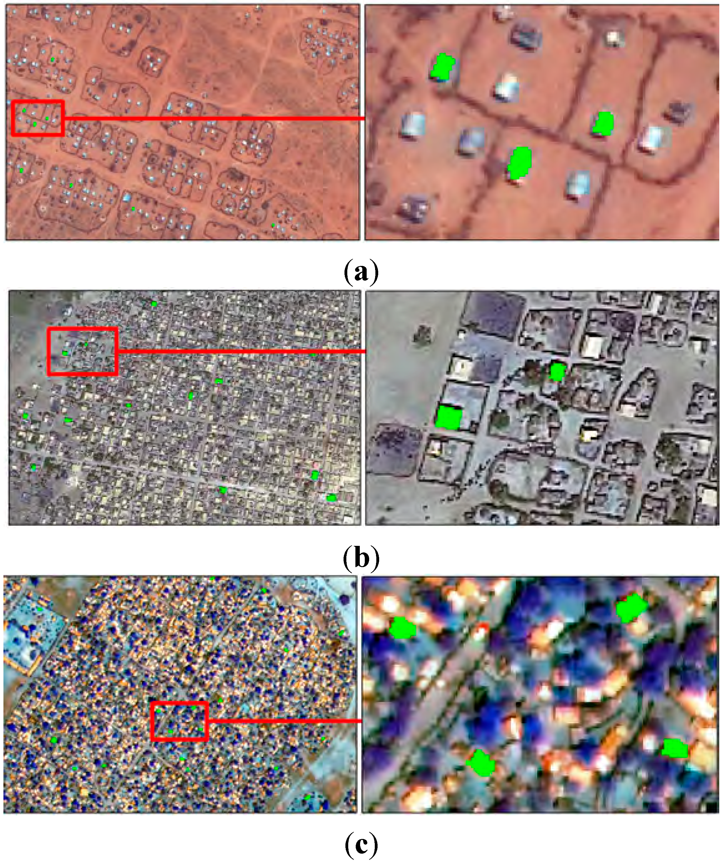
Table 3. The datasets, with accompanying metadata, used for evaluating the method variants (adapted from [6]).

Test Site	Target Elements	Sensor	Spatial Resolution	Reference Segments	Channels	Date Captured
Bokolmanyo 1	Tents	GeoEye-1	0.5 m	28	1, 2, 3	24/8/2011
Jowhaar 1	Structures	GeoEye-1	0.5 m	40	1, 2, 3	26/02/2011
Hagadera 2	Structures	WorldView-2	0.5 m	38	4, 6, 3	07/10/2010

¹ GeoEye, Inc.^© 2011, provided by e-GEOS S.p.A., under GSC-DA, all rights reserved.; ² DigitalGlobe, Inc.^© 2010, provided by EUSI under EC/ESA/GSC-DA, all rights reserved.

Table 3. The datasets, with accompanying metadata, used for evaluating the method variants (adapted from [6]).

Test Site	Target Elements	Sensor	Spatial Resolution	Reference Segments	Channels	Date Captured
Bokolmanyo 1	Tents	GeoEye-1	0.5 m	28	1, 2, 3	24/8/2011
Jowhaar 1	Structures	GeoEye-1	0.5 m	40	1, 2, 3	26/02/2011
Hagadera 2	Structures	WorldView-2	0.5 m	38	4, 6, 3	07/10/2010

¹ GeoEye, Inc.^© 2011, provided by e-GEOS S.p.A., under GSC-DA, all rights reserved.; ² DigitalGlobe, Inc.^© 2010, provided by EUSI under EC/ESA/GSC-DA, all rights reserved.

5. Experimental Evaluation

The presented method is firstly analyzed to verify that it constitutes a multidimensional search problem with parameter interdependencies measured among all constitute components (Section 5.1). A range of common metaheuristics is then tested on the method, evaluating the merits of using more complex search methods compared with simpler search strategies (Section 5.2). Finally an extensive relative comparison is conducted (Section 5.3) on the four method variants under a variety of metric and problem conditions. The merits of the variants are highlighted via measuring computing costs and generating a statistical ranking under cross-validated conditions.

5.1. Parameter Interdependencies

The parameters of the CC + Attr + Map method variant, specifically using the GT function for mapping, are profiled for interdependencies using a statistical parameter interdependency test. Without interdependencies among constituents, such a multidimensional problem may be decomposed into smaller, independently solvable problems. The test, able to profile the frequency of parameter interdependencies [59], is briefly described.

A given parameter ${\text{x}}_{\text{i}}$ is affected by another ${\text{x}}_{\text{j}}$ if a change in the ordering of solution finesses is observed by independently varying values for ${\text{x}}_{\text{i}}$ and ${\text{x}}_{\text{j}}$ in arbitrary full parameter sets ($\text{a},\text{b}$). Formally, ${\text{x}}_{\text{i}}$ is affected by ${\text{x}}_{\text{j}}$ if

$$\begin{gathered} f(a)\le f(b) \& f(a\prime )>f(b\prime ) with \\ a=(\dots ,x\_i,\dots ,x\_j,\dots ) \\ b=(\dots ,x\_i\prime ,\dots ,x\_j,\dots ) \\ a\prime =(\dots ,x\_i,\dots ,x\_j\prime ,\dots ) \\ b\prime =(\dots ,x\_i\prime ,\dots ,x\_j\prime ,\dots ) \end{gathered}$$

(7)

where the function f is the RWJ measure in this implementation.

This test may be repeated multiple times to generate an indication of the frequency of parameter interaction. A table may be generated, with the parameters labeled in the first column denoted as being affected by the parameters listed in the first row, if a value above zero is generated.

The parameter interdependency test is repeated 100 times for each parameter pair, using the CC + Attr + Map method variant for all three problems. The RWJ metric was used to judge a change in segment quality. Note that the metric can measure notions of over- and under-segmentation. Table 4, Table 5 and Table 6 report the number of affected cases for all parameters over the allocated 100 runs. For each problem having differing characteristics, both the parameters of the CC algorithm are shown with a random selection of parameters investigated for the GT mapping function and attribute thresholds. A method constituent (vertically listed “Mapping function”, “CC parameters” and “Attributes”) will be considered unaffected by another constituent (horizontally listed) if all values within the given sub-division are zero.

In all three problems, all parameter constituents are affected by all other constituents. The degree of interaction ranges from frequent, e.g., in the case of CC parameters and attribute thresholds affected by mapping function parameters, to very infrequent, such as in the case of the CC parameters affected by attribute thresholds. Generally, the investigated mapping function parameter affects other parameters most frequently. Interaction is present in all cases. This validates the presented method as a singular optimization problem. Note that the magnitude of the variation in solution quality is not recorded in these tests. Relative solution qualities are investigated in Section 5.3. Interestingly, note that the global range parameter is commonly affected more by the local range parameter (than vice versa), even though modifying the local range parameter beyond the value of the global range parameter has no effect [10].

Table 4. Interdependency test of the method constituents for the Bokolmanyo problem. Note that all constituents affect one another. The mapping function affects all parameters most frequently.

Bokolmanyo		Mapping Function			CC		Attributes
		GT1	GT2	GT10	Local	Global	Area	Std	CH2
Mapping function	GT1		15	19	2	0	3	0	2
	GT2	36		29	3	0	2	3	2
	GT10	38	12		4	0	2	1	3
CC	Local	6	13	11		1	2	0	1
	Global	31	15	24	12		6	0	2
Attributes	Area	19	28	22	2	1		0	3
	Std	21	25	32	1	1	11		2
	CH2	13	11	9	1	0	1	0

Table 4. Interdependency test of the method constituents for the Bokolmanyo problem. Note that all constituents affect one another. The mapping function affects all parameters most frequently.

Bokolmanyo		Mapping Function			CC		Attributes
		GT1	GT2	GT10	Local	Global	Area	Std	CH2
Mapping function	GT1		15	19	2	0	3	0	2
	GT2	36		29	3	0	2	3	2
	GT10	38	12		4	0	2	1	3
CC	Local	6	13	11		1	2	0	1
	Global	31	15	24	12		6	0	2
Attributes	Area	19	28	22	2	1		0	3
	Std	21	25	32	1	1	11		2
	CH2	13	11	9	1	0	1	0

Table 5. Interdependency test of the method constituents for the Jowhaar problem.

Jowhaar		Mapping Function			CC		Attributes
		GT3	GT4	GT9	Local	Global	Perim	Smooth	CH1
Mapping function	GT3		33	20	3	0	1	0	1
	GT4	8		9	4	0	0	1	0
	GT9	19	34		4	2	1	1	1
CC	Local	13	16	11		7	0	2	0
	Global	17	18	20	12		10	0	4
Attributes	Perm	20	24	18	2	3		1	6
	Smooth	8	3	2	1	0	0		0
	CH1	12	14	16	2	0	5	1

Table 5. Interdependency test of the method constituents for the Jowhaar problem.

Jowhaar		Mapping Function			CC		Attributes
		GT3	GT4	GT9	Local	Global	Perim	Smooth	CH1
Mapping function	GT3		33	20	3	0	1	0	1
	GT4	8		9	4	0	0	1	0
	GT9	19	34		4	2	1	1	1
CC	Local	13	16	11		7	0	2	0
	Global	17	18	20	12		10	0	4
Attributes	Perm	20	24	18	2	3		1	6
	Smooth	8	3	2	1	0	0		0
	CH1	12	14	16	2	0	5	1

Table 6. Interdependency test of the method constituents for the Hagadera problem.

Hagadera		Mapping Function			CC		Attributes
		GT6	GT7	GT8	Local	Global	CH3	CH4	CH5
Mapping function	GT6		27	15	3	3	3	1	3
	GT7	29		25	5	1	4	1	2
	GT8	23	33		7	4	1	0	1
CC	Local	10	7	9		4	3	1	4
	Global	27	13	20	6		4	0	0
Attributes	CH3	6	3	3	0	0		1	4
	CH4	4	3	2	0	0	0		0
	CH5	3	2	0	0	0	1	0

Table 6. Interdependency test of the method constituents for the Hagadera problem.

Hagadera		Mapping Function			CC		Attributes
		GT6	GT7	GT8	Local	Global	CH3	CH4	CH5
Mapping function	GT6		27	15	3	3	3	1	3
	GT7	29		25	5	1	4	1	2
	GT8	23	33		7	4	1	0	1
CC	Local	10	7	9		4	3	1	4
	Global	27	13	20	6		4	0	0
Attributes	CH3	6	3	3	0	0		1	4
	CH4	4	3	2	0	0	0		0
	CH5	3	2	0	0	0	1	0

For illustrative purposes, Figure 8 shows exhaustive fitness calculations (RWJ metric) for arbitrary two-dimensional slices of the parameter space (also called the search surface). Figure 8a shows the interaction of the local range parameter of the CC algorithm interacting with the B1 parameter of the spectral split mapping function. Note two local optima. All other parameters were given initial random values and were kept constant during the generation of the search surface. Figure 8b illustrates similarly, with a simpler interaction (single optimal) between thresholds of the CH1 attribute and the local range parameter of CC. Note that these figures are illustrative of parameter interactions and may be vastly different (more complex/less complex) under different external parameter conditions.

5.2. Search Surface Complexity

In Section 5.1, it was shown that parameter interactions exist in the presented method. Some interactions are frequent in the case of selected constituents. Here we investigate the applicability [39] of a range of search methods to traverse the search surfaces of the four method variants. Intuitively the CC variant of the method, with a relatively simple interaction between the local and global range parameters, would not be a difficult search problem. Simple parameter tuning would be feasible in such a scenario using the CC variant of the method, or a simple grid search or random parameter search.

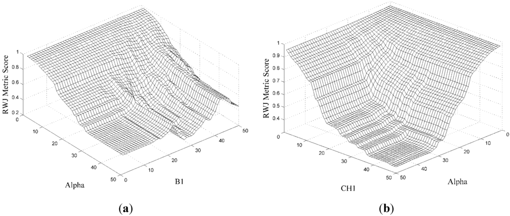
Figure 8. Two-dimensional parameter plots, or search surfaces, demonstrating parameter interactions between method constituents: (a) illustrates the interaction of the alpha parameter from the CC constituent and that of a mapping function parameter, while (b) shows the interaction of alpha with the CH1 attribute.

Figure 8. Two-dimensional parameter plots, or search surfaces, demonstrating parameter interactions between method constituents: (a) illustrates the interaction of the alpha parameter from the CC constituent and that of a mapping function parameter, while (b) shows the interaction of alpha with the CH1 attribute.

The four method variants are run on the Bokolmanyo problem (GT mapping), conjectured to exhibit the simplest search surfaces. Four search methods, namely random search (RND), HillClimber (HC), standard particle swarm optimization (PSO), and a standard variant of Differential Evolution (DE) are investigated (Section 2.3). The RWJ metric is used to judge segment quality. The search process is granted 2000 iterations. Thus, although the tested search methods have vastly different mechanisms (single or population-based, stochastic or deterministic), they are evaluated based on an equal computing budget. Each experiment is repeated 20 times. Averages over the 20 runs are quoted, with the standard deviations also given. The CC method variant has a two-dimensional parameter domain, the CC + Attr variant 12 dimensions, CC + Map also 12 and the CC + Attr + Map method variant 22. Cross-validation was not performed, as search method progress and feasibility were evaluated.

Table 7 lists the optimal achieved metric scores (RWJ) given 2000 search method iterations. The shaded cells indicate the search methods achieving the best scores for each method variant. Various ties in optimal results among the search methods are noted. Firstly, on examining the CC method variant, as expected, no benefit is seen from using more complex search methods. Note that even on this simple search surface, the HC method could not find the global optimal routinely. Similarly, adding attribute thresholding as additional parameters (CC + Attr) gave similar results across the different search methods. Again, HC performed worse than the other methods. In these two method variants, RND, PSO, and DE routinely generated the optimal results. Note that initialization of the parameters in the search processes was random (as opposed to, for example, distributed hypercube sampling). Interestingly, none of the search methods was able to find optimal values on the edge of the search domain when attributes were introduced (owing to random initialization).

Table 7. Performance of the four search methods on the four method variants. In the simpler CC method variants (CC and CC + Attr), no benefit is noted from using more advanced search methods. In the case of the higher dimensional method variants (CC + Map and CC + Attr + Map), using an advanced search method becomes necessary.

	CC	CC + Attr	CC + Map	CC + Attr + Map
RND	0.429 ± 0.000	0.448 ± 0.000	0.186 ± 0.012	0.193 ± 0.015
HC	0.442 ± 0.009	0.535 ± 0.144	0.507 ± 0.083	0.538 ± 0.159
PSO	0.429 ± 0.000	0.448 ± 0.000	0.167 ± 0.012	0.163 ± 0.008
DE	0.429 ± 0.000	0.448 ± 0.000	0.161 ± 0.003	0.163 ± 0.003

Table 7. Performance of the four search methods on the four method variants. In the simpler CC method variants (CC and CC + Attr), no benefit is noted from using more advanced search methods. In the case of the higher dimensional method variants (CC + Map and CC + Attr + Map), using an advanced search method becomes necessary.

	CC	CC + Attr	CC + Map	CC + Attr + Map
RND	0.429 ± 0.000	0.448 ± 0.000	0.186 ± 0.012	0.193 ± 0.015
HC	0.442 ± 0.009	0.535 ± 0.144	0.507 ± 0.083	0.538 ± 0.159
PSO	0.429 ± 0.000	0.448 ± 0.000	0.167 ± 0.012	0.163 ± 0.008
DE	0.429 ± 0.000	0.448 ± 0.000	0.161 ± 0.003	0.163 ± 0.003

Considering the CC + Map and CC + Attr + Map variants of the method, the more complex search methods (PSO, DE) performed substantially better (statistically significantly different, Student’s t-test with a 95% confidence interval) than the RND and especially the HC search method. A difference in 0.030 in the case of the RWJ metric when results approach their optimum is in a practical sense very noticeable. This suggests that under the higher dimensional problem conditions, with more complexities introduced by a mapping function, stochastic population-based search strategies (or others) are needed. Note the slight decrease in standard deviation in the most complex method variants. Also, as generally documented [60], the generic variant of DE performed slightly better than the generic variant of PSO. Further results are presented exclusively with the DE method.

Figure 9 shows the search progress profiles over the allocated 2000 iterations (averaged over 20 runs) for the CC (Figure 9a), CC + Attr (Figure 9b), CC + Map (Figure 9c), and CC + Attr + Map (Figure 9d) method variants. Note that in the simpler method variants (CC and CC + Attr), the optimal results are achieved within 100 method iterations. The more complex method variants (CC + Map and CC + Attr + Map) need substantially more search iterations to achieve optimal or near-optimal results. Figure 9c,d also shows that under the more complex problem formulations, PSO and DE provide better results relatively early on in the search process, suggesting their use even under constrained processing conditions. These plots reveal that method termination may be suggested at around 1000 iterations in these method formulations, or an alternative termination condition may be encoded based on derivatives observed between 500 and 1000 iterations.

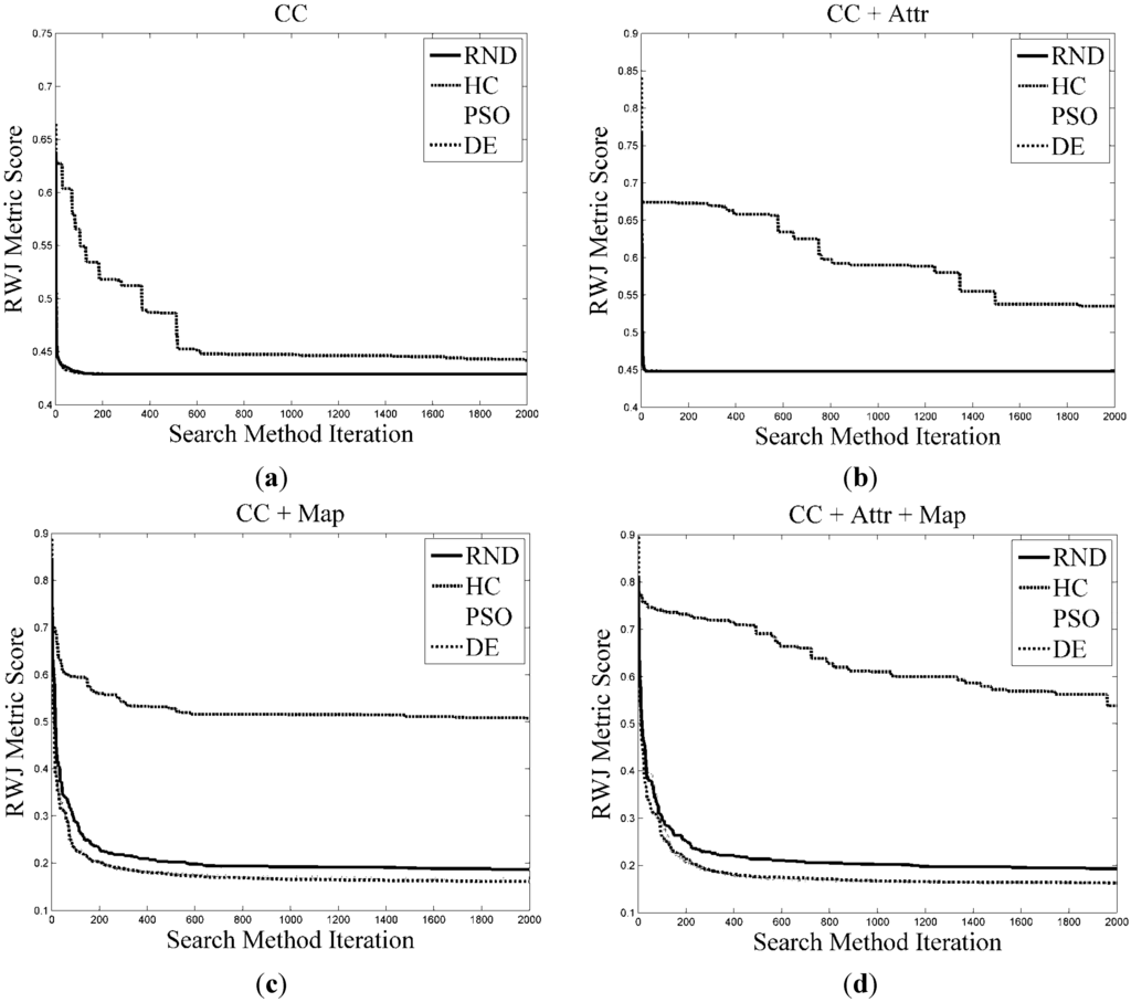
Figure 9. Search method profiles for the four method variants, namely CC (a), CC + Attr (b), CC + Map (c), and CC + Attr + Map (d). Note the increased performance of DE and PSO when considering the CC + Map and CC + Attr + Map method variants.

Figure 9. Search method profiles for the four method variants, namely CC (a), CC + Attr (b), CC + Map (c), and CC + Attr + Map (d). Note the increased performance of DE and PSO when considering the CC + Map and CC + Attr + Map method variants.

5.3. Method Variant Performances

The four presented method variants are evaluated, relative to one another, based on maximal achieved metric scores under cross-validated conditions. Profiling such relative performances in general may give an indication of the merits of the constituents in such a framework. Computing times are also contrasted, as well as convergence behavior, which are important considerations to reduce method processing times. For each problem (Bokolmanyo, Jowhaar, Hagadera), the four method variants are run using all three detailed empirical discrepancy metrics. Each experiment is repeated 20 times, with averages and standard deviations reported. For each site a random mapping function was selected (SS, LIN, or GT). In addition, the best results obtained during the 20 runs are also reported. Thus for each method variant, nine differentiated segmentation tasks (problem type, metric characteristic) are evaluated with over 50 million individual segment evaluations conducted.

Table 8, Table 9 and Table 10 list the achieved metric scores for the problems under different metric and method variant conditions. Note that method variants may be contrasted based on a given metric and not via different metric values. On examining Table 8, depicting the Bokolmanyo problem, it is clear that the more elaborate method variants employing a mapping function (LIN in this case) and a mapping function plus attributes generated superior results compared with the CC and CC + Attr variants. Interestingly, under cross-validated conditions, the addition of constraining attributes (CC + Attr) created an overfitting scenario, resulting in worse performances compared with not employing constraining attributes.

The performances of CC + LIN and CC + Attr + LIN are similar, with the given metric dictating the superior method. Under the RBSB metric condition the CC + LIN method variant displays extremely sporadic results. This suggests that the search surfaces generated under this condition contain numerous discontinuities, creating difficulties for the DE search method. This may be due to the formulation, or nature, of RBSB. It is reference segment centric. In contrast, considering the CC + Attr method variant, the RBSB metric proved robust and similar to the CC variant in terms of optimal results.

Table 8. Method performance on the Bokolmanyo problem. Note the improved results with the CC + LIN and CC + Attr + LIN method variants under all metric conditions.

		CC	CC + Attr	CC + LIN	CC + Attr + LIN
RWJ	Avg	0.465 ± 0.000	0.520 ± 0.035	0.239 ± 0.020	0.235 ± 0.026
	Min	0.465	0.476	0.211	0.200
RBSB	Avg	0.299 ± 0.000	0.308 ± 0.009	0.262 ± 0.235	0.185 ± 0.034
	Min	0.299	0.301	0.136	0.144
PD_OCE	Avg	0.538 ± 0.009	0.556 ± 0.030	0.233 ± 0.016	0.244 ± 0.026
	Min	0.526	0.514	0.199	0.205

Table 8. Method performance on the Bokolmanyo problem. Note the improved results with the CC + LIN and CC + Attr + LIN method variants under all metric conditions.

		CC	CC + Attr	CC + LIN	CC + Attr + LIN
RWJ	Avg	0.465 ± 0.000	0.520 ± 0.035	0.239 ± 0.020	0.235 ± 0.026
	Min	0.465	0.476	0.211	0.200
RBSB	Avg	0.299 ± 0.000	0.308 ± 0.009	0.262 ± 0.235	0.185 ± 0.034
	Min	0.299	0.301	0.136	0.144
PD_OCE	Avg	0.538 ± 0.009	0.556 ± 0.030	0.233 ± 0.016	0.244 ± 0.026
	Min	0.526	0.514	0.199	0.205

The Jowhaar problem (Table 9) displays a slightly different general trend. Under all metric conditions the mapping function method variant (CC + SS) proved superior to both the attribute (CC + Attr) and combined mapping function and attribute (CC + Attr + SS) method variants. Under cross-validated conditions, no benefit was seen from employing attributes, commonly leading to worse results. Note that generally the absolute results were poorer compared with the easier Bokolmanyo problem.

Table 9. Method performance on the Jowhaar problem. The method variant employing a data mapping function (CC + SS) performed the best under all metric conditions.

		CC	CC + Attr	CC + SS	CC + Attr + SS
RWJ	Avg	0.551 ± 0.003	0.784 ± 0.001	0.411 ± 0.009	0.757 ± 0.013
	Min	0.548	0.783	0.392	0.739
RBSB	Avg	0.622 ± 0.000	0.652 ± 0.003	0.418 ± 0.058	0.616 ± 0.023
	Min	0.622	0.649	0.348	0.581
PD_OCE	Avg	0.684 ± 0.002	0.825 ± 0.006	0.549 ± 0.032	0.807 ± 0.021
	Min	0.683	0.816	0.506	0.769

Table 9. Method performance on the Jowhaar problem. The method variant employing a data mapping function (CC + SS) performed the best under all metric conditions.

		CC	CC + Attr	CC + SS	CC + Attr + SS
RWJ	Avg	0.551 ± 0.003	0.784 ± 0.001	0.411 ± 0.009	0.757 ± 0.013
	Min	0.548	0.783	0.392	0.739
RBSB	Avg	0.622 ± 0.000	0.652 ± 0.003	0.418 ± 0.058	0.616 ± 0.023
	Min	0.622	0.649	0.348	0.581
PD_OCE	Avg	0.684 ± 0.002	0.825 ± 0.006	0.549 ± 0.032	0.807 ± 0.021
	Min	0.683	0.816	0.506	0.769

The Hagadera problem (Table 10), considered the most difficult problem, exhibits curious results not corroborating trends observed in the previous two problems. Under different metric conditions, the three method variants (CC + Attr, CC + GT, and CC + Attr + GT) all achieved the top performance. CC + GT was superior under the RWJ metric condition, CC + Attr under the RBSB condition, and CC + Attr + GT under the PD_OCE condition.

Table 10. Method performances on the Hagadera problem. The top performing method variant is metric dependent.

		CC	CC + Attr	CC + GT	CC + Attr + GT
RWJ	Avg	0.614 ± 0.000	0.631 ± 0.008	0.492 ± 0.013	0.509 ± 0.012
	Min	0.614	0.619	0.468	0.494
RBSB	Avg	0.737 ± 0.000	0.511 ± 0.014	1.633 ± 1.061	0.522 ± 0.045
	Min	0.737	0.486	0.526	0.460
PD_OCE	Avg	0.705 ± 0.001	0.684 ± 0.005	0.617 ± 0.023	0.616 ± 0.028
	Min	0.704	0.678	0.579	0.553

Table 10. Method performances on the Hagadera problem. The top performing method variant is metric dependent.

		CC	CC + Attr	CC + GT	CC + Attr + GT
RWJ	Avg	0.614 ± 0.000	0.631 ± 0.008	0.492 ± 0.013	0.509 ± 0.012
	Min	0.614	0.619	0.468	0.494
RBSB	Avg	0.737 ± 0.000	0.511 ± 0.014	1.633 ± 1.061	0.522 ± 0.045
	Min	0.737	0.486	0.526	0.460
PD_OCE	Avg	0.705 ± 0.001	0.684 ± 0.005	0.617 ± 0.023	0.616 ± 0.028
	Min	0.704	0.678	0.579	0.553

Figure 10 shows some optimal results obtained for various problem runs depicted in Table 8, Table 9 and Table 10. Each sub-figure shows a given reference segment, delineated with a red polyline. Resulting segments for the best performing parameter sets are shown with white polylines. The RWJ metric scores for the specific segment are also quoted. The given metric scores are specific to the red delineated reference segments shown (randomly chosen) and not the averaged and cross-validated results generated during experimentation. Figure 10a–c shows local optimal results for the CC method variant. Figure 10d–f presents the results under the CC + Attr method variant, Figure 10g–i for the CC + Map method variant and Figure 10j–l for the CC + Attr + Map variant. Note the same results generated for the Jowhaar problem under CC and CC + Attr method conditions (Figure 10b,e), with constraining attributes not affecting segment quality over the given reference segment.

Generally, based on observing Table 8, Table 9 and Table 10, the introduction of mapping functions provides more robust improvements under more conditions compared with adding attributes. In some cases a combination of attributes and a mapping function proved most useful. Table 11 lists the average computing times needed for 2000 method evaluations, contrasting the performances of the CC + Map and CC + Attr method variants. Computing attributes requires substantially more computing time (Intel^® Xeon^® E5-2643 3.5 GHz processor with single-core processing). Attribute calculations were done incrementally in the CC framework, which is more efficient than calculating attributes independently for each new level of the local range parameter. The optimal achieved parameter values are also reported. Similar to related work [6], near optimal parameter value combinations exist owing to segmentation algorithm and mapping function characteristics.

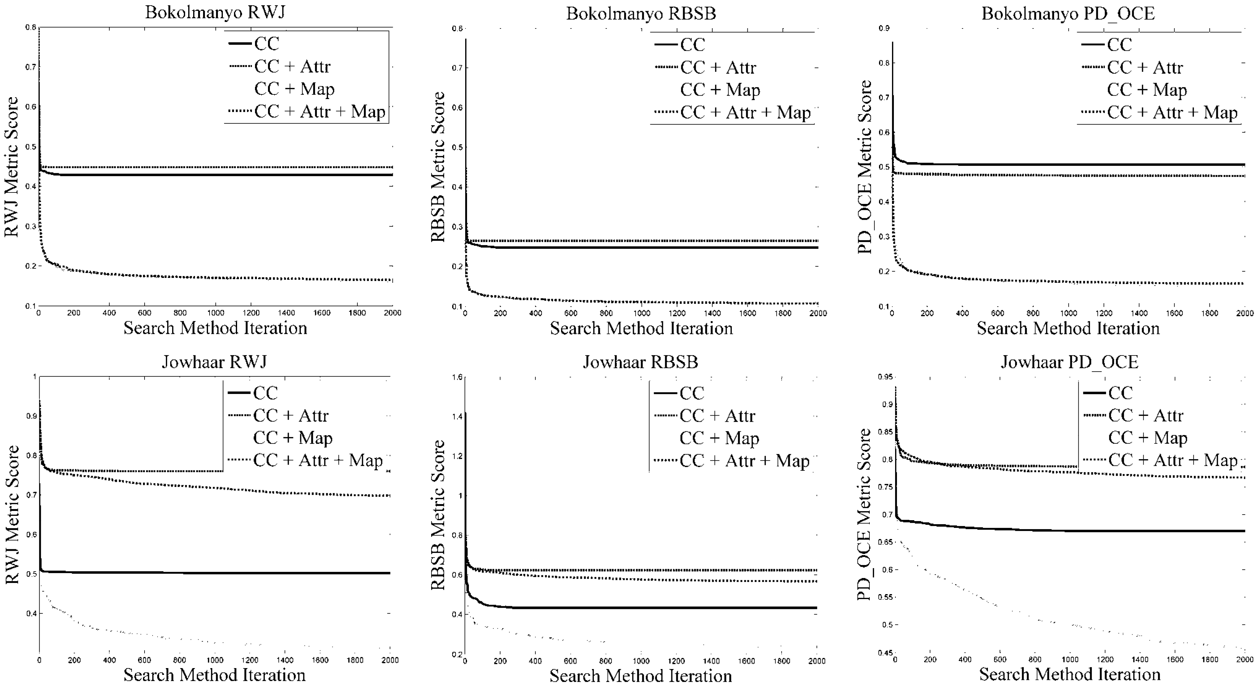
Following on from Table 11, Figure 11 shows the averaged fitness profiles for the various problems and corresponding metrics, prior to cross-validation. Specifically, note the slightly slower start of mapping function method variants compared with attribute variants; however, they ultimately lead to better results (and in the first two problems start off better). In terms of search method progression, some variation exists based on the difficulty of the problem. Generally all variants converged more slowly in the Hagadera problem (“difficult”) compared with the Bokolmanyo problem. Note the variations in optimal results compared with cross-validated values (Table 8, Table 9 and Table 10), specifically considering the RBSB metric with its compact formulation. The figure also highlights the fact that the more complex method variants obtain superior results relatively quickly in the search processes—useful information if method execution times need to be short.

Figure 10. Exemplar optimal segmentation results focused on a random reference segment. The rows depict the CC, CC + Attr, CC + Map, and CC + Attr + Map method variants respectively (in order). The columns denote the three problems, Bokolmanyo, Jowhaar, and Hagadera (in order). (a) RWJ: 0.574; (b) RWJ: 0.524; (c) RWJ: 0.787; (d) RWJ: 0.683; (e) RWJ: 0.524; (f) RWJ: 0.806; (g) RWJ: 0.104; (h) RWJ: 0.506; (i) RWJ: 0.787; (j) RWJ: 0.063; (k) RWJ: 0.437; (l) RWJ: 0.549.

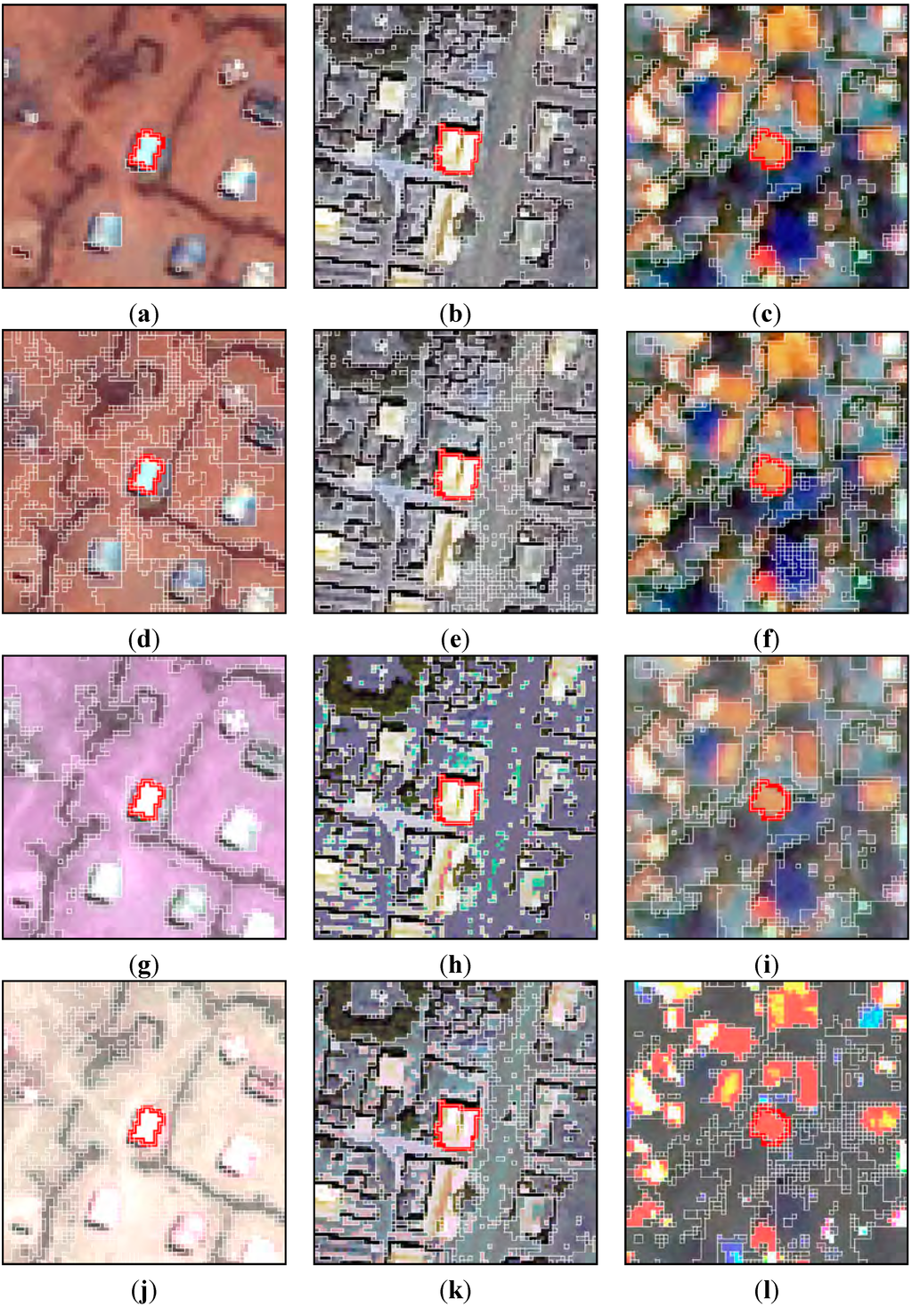
Figure 10. Exemplar optimal segmentation results focused on a random reference segment. The rows depict the CC, CC + Attr, CC + Map, and CC + Attr + Map method variants respectively (in order). The columns denote the three problems, Bokolmanyo, Jowhaar, and Hagadera (in order). (a) RWJ: 0.574; (b) RWJ: 0.524; (c) RWJ: 0.787; (d) RWJ: 0.683; (e) RWJ: 0.524; (f) RWJ: 0.806; (g) RWJ: 0.104; (h) RWJ: 0.506; (i) RWJ: 0.787; (j) RWJ: 0.063; (k) RWJ: 0.437; (l) RWJ: 0.549.

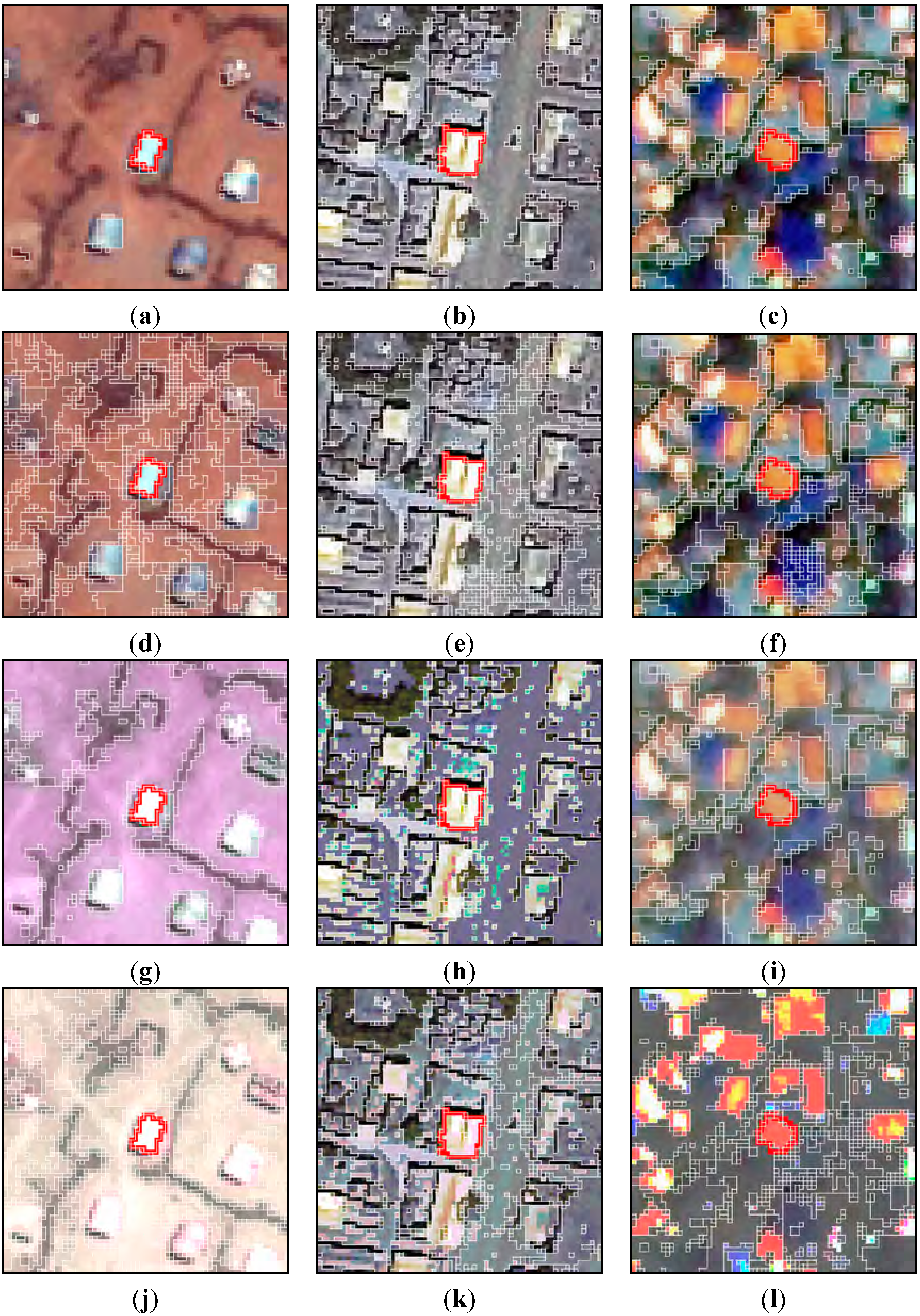
Table 11. Average computing times for experimental runs and resulting method parameters. Note the increased computing time of method variants employing attributes.

Problem	Method Variant	Time	Alpha	WGlobal	Area	Std	Perimeter	Smoothness	Compactness
Bokolmanyo	CC + Map	2062.304 ± 248.996	187.600 ± 68.646	53.600 ± 15.601	NA	NA	NA	NA	NA
	CC + Attr	3083.551 ± 237.328	173.300 ± 66.331	196.000 ± 44.838	247.500 ± 142.417	50.442 ± 58.470	369.900 ± 196.794	21.483 ± 7.688	19.803 ± 7.439
Jowhaar	CC + Map	2182.659 ± 193.999	165.900 ± 82.538	155.200 ± 19.136	NA	NA	NA	NA	NA
	CC + Attr	4136.116 ± 498.270	98.900 ± 52.297	203.500 ± 43.775	392.000 ± 85.249	133.289 ± 60.647	620.500 ± 241.420	18.379 ± 6.910	22.466 ± 4.331
Hagadera	CC + Map	2168.177 ± 226.159	101.700 ± 65.052	148.300 ± 29.803	NA	NA	NA	NA	NA
	CC + Attr	5409.293 ± 352.444	187.400 ± 68.704	240.300 ± 21.525	342.100 ± 81.266	162.601 ± 86.782	574.700 ± 271.998	23.573 ± 7.351	19.940 ± 6.113

Table 11. Average computing times for experimental runs and resulting method parameters. Note the increased computing time of method variants employing attributes.

Problem	Method Variant	Time	Alpha	WGlobal	Area	Std	Perimeter	Smoothness	Compactness
Bokolmanyo	CC + Map	2062.304 ± 248.996	187.600 ± 68.646	53.600 ± 15.601	NA	NA	NA	NA	NA
	CC + Attr	3083.551 ± 237.328	173.300 ± 66.331	196.000 ± 44.838	247.500 ± 142.417	50.442 ± 58.470	369.900 ± 196.794	21.483 ± 7.688	19.803 ± 7.439
Jowhaar	CC + Map	2182.659 ± 193.999	165.900 ± 82.538	155.200 ± 19.136	NA	NA	NA	NA	NA
	CC + Attr	4136.116 ± 498.270	98.900 ± 52.297	203.500 ± 43.775	392.000 ± 85.249	133.289 ± 60.647	620.500 ± 241.420	18.379 ± 6.910	22.466 ± 4.331
Hagadera	CC + Map	2168.177 ± 226.159	101.700 ± 65.052	148.300 ± 29.803	NA	NA	NA	NA	NA
	CC + Attr	5409.293 ± 352.444	187.400 ± 68.704	240.300 ± 21.525	342.100 ± 81.266	162.601 ± 86.782	574.700 ± 271.998	23.573 ± 7.351	19.940 ± 6.113

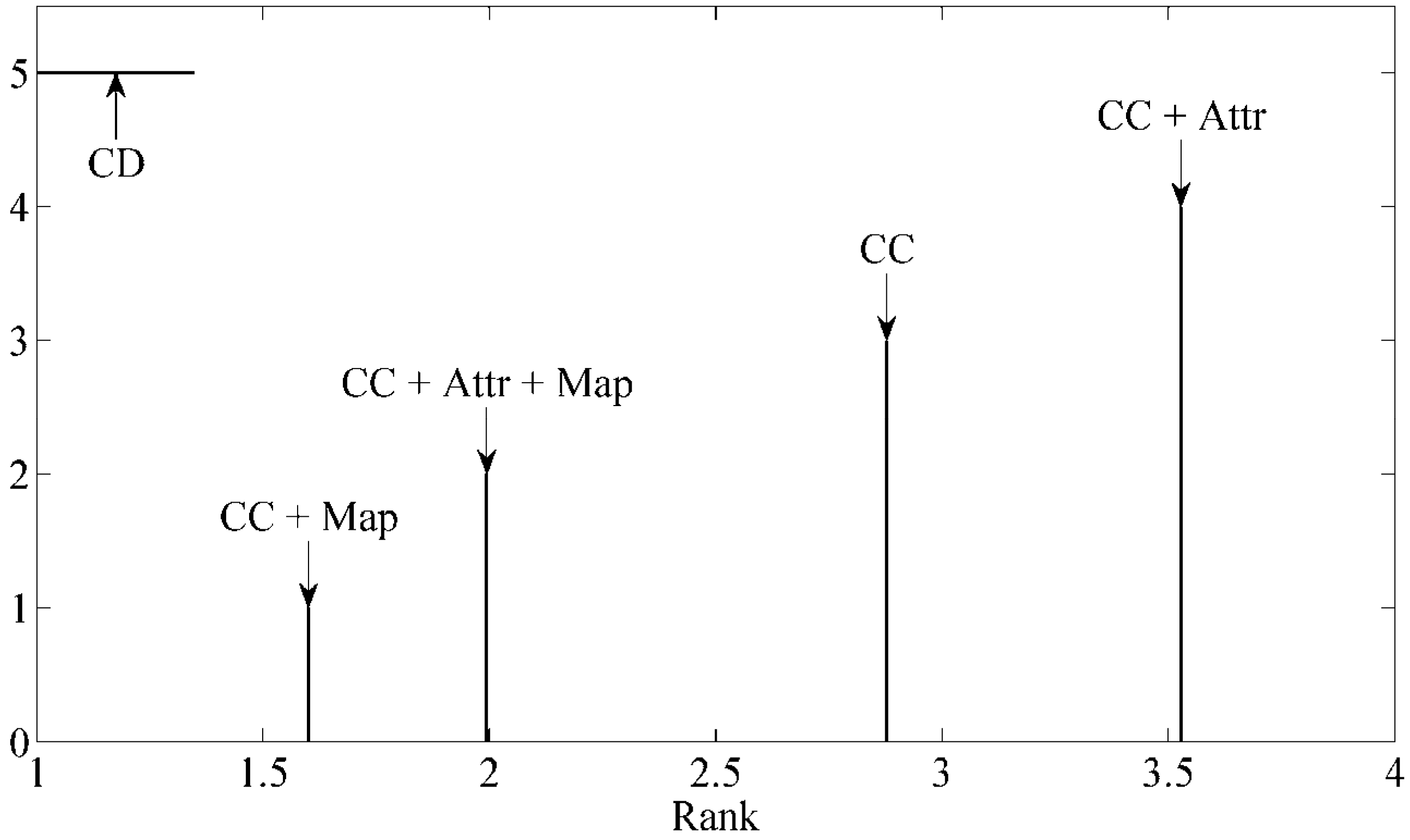
Finally, and most significantly, the results reported in Table 8, Table 9 and Table 10 are augmented with a Friedman rank test [61] to give a generalized and discrete indication of the usefulness of the method variants. The Friedman rank test is a simple non-parametric test ranking multiple methods (e.g., CC, CC + Map, etc.) over multiple problems/data sets. The rank test was run on the four method variants considering the various problems and metric conditions (36 in total, cross-validated). A Nemenyi post hoc test was also conducted to test whether critical differences exist. Figure 12 illustrates this result, with the confidence interval set to 95% and a critical difference of 0.349 (ranking) generated. Note that the figure shows results under cross-validated conditions.

Figure 11. Search method profiles for the different problems under different metric conditions. Note that for the simpler Bokolmanyo problem near-optimal results are achieved relatively early on in the search process. In the more complex problems, the methods need substantially more iterations in finding the achievable optimal parameter set.

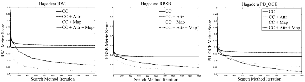
Figure 11. Search method profiles for the different problems under different metric conditions. Note that for the simpler Bokolmanyo problem near-optimal results are achieved relatively early on in the search process. In the more complex problems, the methods need substantially more iterations in finding the achievable optimal parameter set.

On examining Figure 12, the CC + Map variant of the method (using various mapping functions) ranked first, followed by the most complex method variant (CC + Attr + Map). Under cross-validated conditions, adding attributes proves detrimental. The investigated problems are not exhaustive. The variants are all statistically significantly different from one another. This figure reports a general observation under extensive evaluations (50 million segment evaluations). Under a more succinct selection of attributes and problems, attributes may well be more useful. The figure suggests simple data mapping functions should be a worthwhile consideration in method design within this general framework. Mapping functions may be considered (indirect means of changing connectivity type), but other more direct means of defining connectivity (parameterizable) may also prove useful. This is in addition to such a variant requiring less computing time, compared with computing additional attributes.

Figure 12. Friedman rank test with a Nemenyi post hoc test conducted on results from Table 8, Table 9 and Table 10. Confidence interval is set to 95%. A Critical Difference (CD) of 0.349 is generated (ranking). All method variants deliver statistically significant different results. Generally speaking, the CC + Map method variant was found most useful.

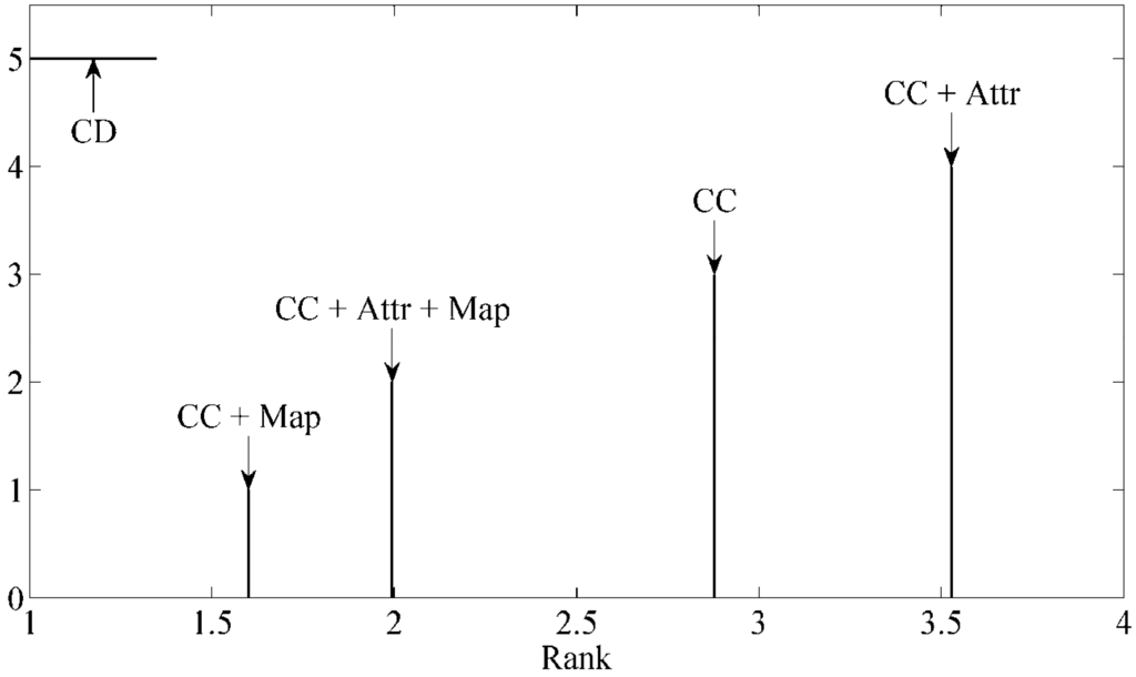
Figure 12. Friedman rank test with a Nemenyi post hoc test conducted on results from Table 8, Table 9 and Table 10. Confidence interval is set to 95%. A Critical Difference (CD) of 0.349 is generated (ranking). All method variants deliver statistically significant different results. Generally speaking, the CC + Map method variant was found most useful.

6. Conclusions

In this work a general method in the context of sample supervised segment generation was examined. Such general methods aim to generate thematically accurate image segments, easing further processing and increasing final classification accuracies. The method incorporates a graph-based segmentation method, with constraining attributes and data mapping functions providing additional flexibility in the nature of the generated segments. These additional constituents to the method were profiled for their relative utility in enhancing the quality of the generated segments. It was found that constraining attributes, conjectured to be useful, did not add value to segment quality. Data mapping functions proved more useful in this regard, generating better quality segments consistently. Other constituents could also be added to such a method, but other formulations of defining connectivity in such an approach could be most beneficial. Various other approaches to changing connectivity could be considered as opposed to mapping functions, including analyzing scene-wide connectivity properties, considering hypo/hyper connectivity definitions, and defining connectedness as part of the optimization problem.

A few experimental considerations should be noted with such a method. Various processes in such a general approach may be stochastic, not only the given metaheuristic. In this particular instance the segmentation algorithm generates unique or repeatable results. This might not always be the case. Adding numerous attributes, without a priori known usefulness, should be avoided as additional search landscape dimensionality increases problem difficulty. Future work could profile a range of spectral and geometric attributes for their usefulness in various problems (land-cover element specific). Using various segment-sampling sizes could also provide additional insight into method generalizability to unseen problems.

A method variant, incorporating attribute selection as part of the optimization problem, could also be considered. This would entail a combined combinatorial and real valued optimization problem. The utilized metrics also need careful consideration, as various metrics will have different convergence characteristics, as shown in this work. The nature of correlations among metric scores and the ease of subsequent processes or classification results are also open to research. Note that the presented method, inherently hierarchical, functions on a singular segmentation level and attempts to find a level appropriate to the given problem or elements of interest in the scene. Hierarchical aspects were not considered.

The proposed method and results add to the discussion on supervised methods for segment generation in a remote sensing context. Applications such as rapid mapping or emergency response mapping may benefit from such approaches. Another application may be targeted land-cover element identification, incorporating single-class classification algorithms. User-driven image analysis approaches, found within the context of Geographic Object Based-Image Analysis (GEOBIA), might benefit from such sample supervised segment generation methods. How methods such as the one presented here, based on modular image segmentation, may efficiently synergize with more complete workflows [62], including classification processes [54,63] or larger automated image analysis methods, should be a worthwhile investigation.

References

- Blaschke, T.; Hay, G.J.; Kelly, M.; Lang, S.; Hofmann, P.; Addink, E.; Feitosa, R.Q.; van der Meer, F.; van der Werff, H.; van Coillie, F.; et al. Geographic object-based image analysis—Towards a new paradigm. ISPRS J. Photogramm. Remote Sens. 2014, 87, 180–191. [Google Scholar] [CrossRef] [PubMed]
- Soille, P.; Pesaresi, M. Advances in mathematical morphology applied to geoscience and remote sensing. IEEE Trans. Geosci. Remote Sens. 2002, 40, 2042–2055. [Google Scholar] [CrossRef]
- Fourie, C.; Schoepfer, E. Connectivity thresholds and data transformations for sample supervised segment generation. In Proceedings of the IEEE International Geoscience and Remote Sensing Symposium (IGARSS 2013), Melbourne, Australia, 21–26 July 2013.
- Bhanu, B.; Lee, S.; Ming, J. Adaptive image segmentation using a genetic algorithm. IEEE Trans. Syst. Man Cybern. 1995, 25, 1543–1567. [Google Scholar] [CrossRef]
- Feitosa, R.Q.; Costa, G.A.O.P.; Cazes, T.B.; Feijo, B. A genetic approach for the automatic adaptation of segmentation parameters. In Proceedings of the Geographic Object-Based Image Analysis (GEOBIA 2006), Salzburg, Austria, 4–5 July 2006.
- Fourie, C.; Schoepfer, E. Data transformation functions for expanded search spaces in geographic sample supervised segment generation. Remote Sens. 2014, 5, 3791–3821. [Google Scholar] [CrossRef]
- Derivaux, S.; Forestier, G.; Wemmert, C.; Lefèvre, S. Supervised image segmentation using watershed transform, fuzzy classification and evolutionary computation. Pattern Recognit. Lett. 2010, 31, 2364–2374. [Google Scholar] [CrossRef]
- Soille, P. Constrained connectivity for hierarchical image partitioning and simplification. IEEE Trans. Pattern Anal. Mach. Intell. 2008, 30, 1132–1145. [Google Scholar] [CrossRef] [PubMed]
- Ouzounis, G.K.; Soille, P. The Alpha-Tree Algorithm; JRC Scientific and Policy Report; Publications Office of the European Union: Luxembourg City, Luxembourg, 2012. [Google Scholar]
- Soille, P. Constrained connectivity for the processing of very-high-resolution satellite images. Int. J. Remote Sens. 2010, 31, 5879–5893. [Google Scholar] [CrossRef]
- Najman, L. On the equivalence between hierarchical segmentations and ultrametric watersheds. J. Math. Imaging Vis. 2011, 40, 231–247. [Google Scholar] [CrossRef]
- Soille, P. Preventing chaining through transitions while favouring it within homogeneous regions. In Mathematical Morphology and Its Applications to Image and Signal Processing; Springer: Berlin, Germany, 2011; pp. 96–107. [Google Scholar]
- Soille, P.; Grazzini, J. Advances in constrained connectivity. In Proceedings of the 14th IAPR International Conference, DGCI 2008, Lyon, France, 16–18 April 2008.
- Gueguen, L.; Soille, P. Frequent and dependent connectivities. In Mathematical Morphology and its Applications to Image and Signal Processing; Springer: Berlin, Germany, 2011; pp. 120–131. [Google Scholar]
- Gueguen, L.; Velasco-Forero, S.; Soille, P. Local mutual information for dissimilarity-based image segmentation. J. Math. Imaging Vis. 2014, 48, 625–644. [Google Scholar] [CrossRef]
- Perret, B.; Lefèvre, S.; Collet, C.; Slezak, É. Hyperconnections and hierarchical representations for grayscale and multiband image processing. IEEE Trans. Image Process. 2012, 21, 14–27. [Google Scholar] [CrossRef] [PubMed]
- Ouzounis, G.K.; Wilkinson, M.H. Hyperconnected attribute filters based on k-flat zones. IEEE Trans. Pattern Anal. Mach. Intell. 2011, 33, 224–239. [Google Scholar] [CrossRef] [PubMed]
- Wilkinson, M.H. An axiomatic approach to hyperconnectivity. In Mathematical Morphology and its Application to Signal and Image Processing; Springer: Berlin, Germany, 2009; pp. 35–46. [Google Scholar]
- Soille, P. Morphological Image Analysis: Principles and Applications; Springer-Verlag: New York, NY, USA, 2003. [Google Scholar]
- Najman, L.; Cousty, J. A graph-based mathematical morphology reader. Pattern Recognit. Lett. 2014, 47, 3–17. [Google Scholar] [CrossRef]
- Tuia, D.; Pacifici, F.; Kanevski, M.; Emery, W.J. Classification of very high spatial resolution imagery using mathematical morphology and support vector machines. IEEE Trans. Geosci. Remote Sens. 2009, 47, 3866–3879. [Google Scholar] [CrossRef]
- Kemper, T.; Jenerowicz, M.; Pesaresi, M.; Soille, P. Enumeration of dwellings in darfur camps from GeoEye-1 satellite images using mathematical morphology. IEEE J. Sel. Top. Appl. Earth Observ. Remote Sens. 2011, 4, 8–15. [Google Scholar] [CrossRef]
- Salembier, P.; Serra, J. Flat zones filtering, connected operators, and filters by reconstruction. IEEE Trans. Image Process. 1995, 4, 1153–1160. [Google Scholar] [CrossRef] [PubMed]
- Breen, E.J.; Jones, R.; Talbot, H. Mathematical morphology: A useful set of tools for image analysis. Stat. Comput. 2000, 10, 105–120. [Google Scholar] [CrossRef]
- Pedergnana, M.; Marpu, P.R.; Dalla Mura, M.; Benediktsson, J.A.; Bruzzone, L. A novel technique for optimal feature selection in attribute profiles based on genetic algorithms. IEEE Trans. Geosci. Remote Sens. 2013, 51, 3514–3528. [Google Scholar] [CrossRef]
- Pesaresi, M.; Benediktsson, J.A. A new approach for the morphological segmentation of high-resolution satellite imagery. IEEE Trans. Geosci. Remote Sens. 2001, 39, 309–320. [Google Scholar] [CrossRef]
- Dalla Mura, M.; Atli Benediktsson, J.; Waske, B.; Bruzzone, L. Extended profiles with morphological attribute filters for the analysis of hyperspectral data. Int. J. Remote Sens. 2010, 31, 5975–5991. [Google Scholar] [CrossRef]
- Fauvel, M.; Benediktsson, J.A.; Chanussot, J.; Sveinsson, J.R. Spectral and spatial classification of hyperspectral data using svms and morphological profiles. IEEE Trans. Geosci. Remote Sens. 2008, 46, 3804–3814. [Google Scholar] [CrossRef]
- Soille, P. On genuine connectivity relations based on logical predicates. In Proceedings of the 14th International Conference on Image Analysis and Processing, Modena, Italy, 10–14 September 2007.
- Wilkinson, M.H.; Roerdink, J.B. Fast morphological attribute operations using tarjan’s union-find algorithm. In Mathematical Morphology and Its Applications to Image and Signal Processing; Springer: Berlin, Germany, 2000; pp. 311–320. [Google Scholar]
- Havel, J.; Merciol, F.; Lefèvre, S. Efficient schemes for computing α-tree representations. In Mathematical Morphology and Its Applications to Image and Signal Processing; Hendriks, C.L., Borgefors, G., Strand, R., Eds.; Springer: Berlin, Germany, 2013; Volume 7883, pp. 111–122. [Google Scholar]
- Neubert, M.; Herold, H.; Meinel, G. Evaluation of remote sensing image segmentation quality—Further results and concepts. Int. Arch. Photogramm. Remote Sens. Spat. Inf. Sci. 2006, 36, 6–11. [Google Scholar]
- Dalla Mura, M.; Benediktsson, J.A.; Bruzzone, L. A general approach to the spatial simplification of remote sensing images based on morphological connected filters. In Proceedings of the IEEE International Geoscience and Remote Sensing Symposium (IGARSS), Vancouver, BC, Canada, 24–29 July 2011.
- Soille, P.; Najman, L. On morphological hierarchical representations for image processing and spatial data clustering. In Applications of Discrete Geometry and Mathematical Morphology; Springer: Berlin, Germany, 2012; pp. 43–67. [Google Scholar]
- Evans, A.N.; Gimenez, D. Extending connected operators to colour images. In Proceedings of the 15th IEEE International Conference on Image Processing, San Diego, CA, USA, 12–15 October 2008.
- Louverdis, G.; Vardavoulia, M.I.; Andreadis, I.; Tsalides, P. A new approach to morphological color image processing. Pattern Recognit. 2002, 35, 1733–1741. [Google Scholar] [CrossRef]
- Talbi, E. Metaheuristics: From Design to Implementation; Wiley: Hoboken, NJ, USA, 2009. [Google Scholar]
- Barr, R.S.; Golden, B.L.; Kelly, J.P.; Resende, M.G.; Stewart, W.R., Jr. Designing and reporting on computational experiments with heuristic methods. J. Heuristics 1995, 1, 9–32. [Google Scholar] [CrossRef]
- Bartz-Beielstein, T. Experimental Research in Evolutionary Computation; Springer: Berlin, Germany, 2006. [Google Scholar]
- Rardin, R.L.; Uzsoy, R. Experimental evaluation of heuristic optimization algorithms: A tutorial. J. Heuristics 2001, 7, 261–304. [Google Scholar] [CrossRef]
- Birattari, M.; Zlochin, M.; Dorigo, M. Towards a theory of practice in metaheuristics design: A machine learning perspective. RAIRO Theor. Inform. Appl. 2006, 40, 353–369. [Google Scholar] [CrossRef]
- Vanneschi, L.; Mussi, L.; Cagnoni, S. Hot topics in evolutionary computation. Intell. Artif. 2011, 5, 5–17. [Google Scholar]
- Pedersen, M. Swarmops: Black-box Optimization in Ansic; Hvass Lab.: Southampton, UK, 2008. [Google Scholar]
- Price, K.V.; Storn, R.M.; Lampinen, J.A. Differential Evolution: A Practical Approach to Global Optimization; Springer: Berlin, Germany, 2005. [Google Scholar]
- Kennedy, J. Particle swarm optimization. In Encyclopedia of Machine Learning; Springer: Berlin, Germany, 2010; pp. 760–766. [Google Scholar]
- Zhang, Y.J. A survey on evaluation methods for image segmentation. Pattern Recognit. 1996, 29, 1335–1346. [Google Scholar] [CrossRef]
- Chabrier, S.; Emile, B.; Rosenberger, C.; Laurent, H. Unsupervised performance evaluation of image segmentation. EURASIP J. Appl. Signal Process. 2006, 2006, 1–12. [Google Scholar] [CrossRef]
- Freddrich, C.M.B.; Feitosa, R.Q. Automatic adaptation of segmentation parameters applied to non-homogeneous object detection. In Proceedings of the Geographic Object-based Image Analysis (GEOBIA), Calgary, AB, Canada, 29 June–2 July 2008.
- Polak, M.; Zhang, H.; Pi, M. An evaluation metric for image segmentation of multiple objects. Image Vis. Comput. 2009, 27, 1223–1227. [Google Scholar] [CrossRef]
- Pignalberi, G.; Cucchiara, R.; Cinque, L.; Levialdi, S. Tuning range image segmentation by genetic algorithm. EURASIP J. Appl. Signal Process. 2003, 2003, 780–790. [Google Scholar] [CrossRef]
- Achanccaray, P.; Ayma, V.; Jimenez, L.; Garcia, S.; Happ, P.; Feitosa, R.; Plaza, A. A free software tool for automatic tuning of segmentation parameters. Southeast. Eur. J. Earth Observ. Geomat. 2014, 3, 707–712. [Google Scholar]
- Cagnoni, S. Evolutionary computer vision: A taxonomic tutorial. In Proceedings of the Eighth International Conference on Hybrid Intelligent Systems (HIS 2008), Barcelona, Spain, 10–12 September 2008.
- Feitosa, R.Q.; Ferreira, R.S.; Almeida, C.M.; Camargo, F.F.; Costa, G.A.O.P. Similarity metrics for genetic adaptation of segmentation parameters. In Proceedings of the Geographic Object-Based Image Analysis (GEOBIA 2010), Ghent, Belgium, 29 June–2 July 2010.
- Fourie, C.; Schoepfer, E. Classifier directed data hybridization for geographic sample supervised segment generation. Remote Sens. 2014, 6, 11852–11882. [Google Scholar] [CrossRef]
- Fourie, C.; Schoepfer, E. Sample supervised search-centric approaches in geographic object-based image analysis (GEOBIA): Concepts, state-of-the-art and a future outlook. In Earth Observation for Land and Emergency Monitoring—Innovative Concepts for Environmental Monitoring from Space; Balzter, H., Ed.; Wiley-Blackwell: Hoboken, NJ, USA, 2015; in press. [Google Scholar]
- Yoda, I.; Yamamoto, K.; Yamada, H. Automatic acquisition of hierarchical mathematical morphology procedures by genetic algorithms. Image Vis. Comput. 1999, 17, 749–760. [Google Scholar] [CrossRef]
- Quintana, M.I.; Poli, R.; Claridge, E. Morphological algorithm design for binary images using genetic programming. Genet. Program. Evol. Mach. 2006, 7, 81–102. [Google Scholar] [CrossRef]
- Gorai, A.; Ghosh, A. Gray-level image enhancement by particle swarm optimization. In Proceedings of the NaBIC 2009 World Congress on Nature & Biologically Inspired Computing, Coimbatore, India, 9–11 December 2009.
- Sun, L.; Yoshida, S.; Cheng, X.; Liang, Y. A cooperative particle swarm optimizer with statistical variable interdependence learning. Inf. Sci. 2012, 186, 20–39. [Google Scholar] [CrossRef]
- Vesterstrom, J.; Thomsen, R. A comparative study of differential evolution, particle swarm optimization, and evolutionary algorithms on numerical benchmark problems. In Proceedings of the CEC2004 Congress on Evolutionary Computation, Portland, OR, USA, 19–23 June 2004.
- Li, Y. Sparse Machine Learning Models in Bioinformatics. Ph.D. Thesis, University of Windsor, Windsor, ON, Canada, 2013. [Google Scholar]
- Baatz, M.; Hoffman, C.; Willhauck, G. Progressing from object-based to object-oriented image analysis. In Object-Based Image Analysis: Spatial Concepts for knowledge-Driven Remote Sensing Applications; Blaschke, T., Lang, S., Hay, G.J., Eds.; Springer: Berlin, Germany, 2008; pp. 29–42. [Google Scholar]
- Mylonas, S.; Stavrakoudis, D.; Theocharis, J.; Mastorocostas, P. A region-based genesis segmentation algorithm for the classification of remotely sensed images. Remote Sens. 2015, 7, 2474–2508. [Google Scholar] [CrossRef]
© 2015 by the authors; licensee MDPI, Basel, Switzerland. This article is an open access article distributed under the terms and conditions of the Creative Commons Attribution license (http://creativecommons.org/licenses/by/4.0/).