Article

Improved Topographic Normalization for Landsat TM Images by Introducing the MODIS Surface BRDF

1
College of Geography and Environment Science, Northwest Normal University, Lanzhou 730070, China
2
Key Laboratory of Remote Sensing of Gansu Province, Cold and Arid Regions Environmental and Engineering Research Institute, Chinese Academy of Sciences, Lanzhou 730000, China
3
Chinese Academy of Sciences (CAS) Center for Excellence in Tibetan Plateau Earth Sciences, Chinese Academy of Sciences, Beijing 100101, China
4
State Key Laboratory of Remote Sensing Science, Institute of Remote Sensing and Digital Earth of Chinese Academy of Sciences, Beijing 100101, China
5
State Key Laboratory of Remote Sensing, School of Geography, Beijing Normal University, Beijing 100875, China
*
Author to whom correspondence should be addressed.
Remote Sens. 2015, 7(6), 6558-6575; https://doi.org/10.3390/rs70606558
Submission received: 5 January 2015 / Revised: 1 May 2015 / Accepted: 4 May 2015 / Published: 26 May 2015

Abstract

:
In rugged terrain, the accuracy of surface reflectance estimations is compromised by atmospheric and topographic effects. We propose a new method to simultaneously eliminate atmospheric and terrain effects in Landsat Thematic Mapper (TM) images based on a 30 m digital elevation model (DEM) and Moderate Resolution Imaging Spectroradiometer (MODIS) atmospheric products. Moreover, we define a normalized factor of a Bidirectional Reflectance Distribution Function (BRDF) to convert the sloping pixel reflectance into a flat pixel reflectance by using the Ross Thick-Li Sparse BRDF model (Ambrals algorithm) and MODIS BRDF/albedo kernel coefficient products. Sole atmospheric correction and topographic normalization were performed for TM images in the upper stream of the Heihe River Basin. The results show that using MODIS atmospheric products can effectively remove atmospheric effects compared with the Fast Line-of-Sight Atmospheric Analysis of Spectral Hypercubes (FLAASH) model and the Landsat Climate Data Record (CDR). Moreover, superior topographic effect removal can be achieved by considering the surface BRDF when compared with the surface Lambertian assumption of topographic normalization.

1. Introduction

Optical remote sensing has been widely used to quantitatively estimate surface parameters [1,2,3], such as various biogeophysical (e.g., leaf area index (LAI)) and geophysical parameters (e.g., albedo). Landsat imagery has been used extensively for quantitatively evaluating surface parameters [4]. However, the satellite-obtained top-of-atmosphere (TOA) radiance is reflected via complex interactions between (1) atmospheric attenuation; (2) incoming solar irradiance at a given surface point, and (3) the surface bidirectional reflectance distribution function (BRDF). In rugged terrain, variations in surface elevation, slope, aspect, the obstruction coefficient, the sky view factor and the topographic configuration factor can significantly impactthese three factors, which produce atmospheric effects, illumination effects, and BRDF effects in optical high-resolution satellite images [5]. Therefore, topographic normalization of satellite imagery has become a prerequisite for retrieving surface parameters, which can reduce or remove atmospheric, topographic and BRDF effects in rugged terrain simultaneously.
The quantitative topographic normalization of Landsat imagery has a relatively long history with the aid of a digital elevation model (DEM).The complexity and difficulty lie in the quantitative simultaneous estimation of the incident radiation, atmospheric transmittance, and surface BRDF for each image pixel in mountainous areas. Earlier studies removed atmospheric effects only by estimating atmospheric parameters, such as aerosols and water vapor, using a radiative transfer equation with a Lambertian surface, as reviewed in the literature [6,4]. Masek et al. [7] derived the Landsat surface reflectance product by atmospheric correction based on the 6S methodology, which is the basis of the Landsat Climate Data Record (CDR) distributed by USGS. Some researchers recognize that the radiance received by the satellite is also distorted due to the surface BRDF or sun-surface-sensor geometry for each image pixel, and several atmospheric-correction-coupled BRDFs are utilized for Landsat images [8]. In recent years, with the development of moderate-resolution satellites, many space-based sensors (such as the Moderate Resolution Imaging Spectroradiometer, MODIS) provide atmospheric products and multi-angle observations, which yield reliable data on land surface BRDFs [9,10]. Some researchers use MODIS atmospheric and BRDF model parameters for Landsat correction [11,12]. However, in mountainous areas, the topography strongly influences the radiance distribution recorded by optical sensors [13]. For the same land surface characteristics, radiance values on a sunny slope are brighter than that those on a shady slope in images [1,5].Since the 1970s, two main categories of topographic correction methods, empirical and physical topographic corrections, have been developed to eliminate or at least reduce topographic influences [14,15]. The first category mainly corrects the solar direct radiance to decrease illumination differences caused by terrain, such as ratio models, cosine models, Minnaert models, sun-canopy-sensor (SCS) models, and C models. Some studies compare several empirical topographic correction approaches for Landsat images [16,17,18,19].These empirical methods are extremely simple and, in particular cases, highly effective; however, they are not suitable for retrieving quantitative surface parameters [5]. The second category employs a radiative transfer code to obtain deterministic descriptions of the correction of topographic effects and avoids image dependence [20].
Some investigators have developed complex terrain factors to describe solar illumination obtained by slope pixels, such as slope inclination, aspect, sky view factor and shadowing effects for radiation from the sky and terrain [21,22,23,24,25]. Moreover, the spatial distribution of atmospheric transmissivity and optical depth vary with the rapidly changing elevation, aerosol optical depth (AOD) and precipitable water (PW); thus, topographic and atmospheric corrections must be performed simultaneously pixel by pixel [15,26,27]. In addition, surface anisotropy, which is a function of the view and illumination angles, is evident. The models with Lambertian assumptions only consider the variation in the actual incident angles caused by the terrain and do not eliminate the influence of real sensor viewing angles [28]. Some researchers have used an empirical BRDF to reduce the high reflectance values in regions of low illumination [13,27,29,30]. In recent years, many quantitative topographic normalization schemes for removing atmospheric, topographic and BRDF effects on Landsat imagery have been proposed using MODIS BRDF parameters [1,2,5]. However, Schaaf et al. [31] discovered that sloping and flat surfaces with similar vegetation have different BRDF shapes that are not symmetrical about the principal plane in rugged terrain. Therefore, to retrieve the surface reflectance from optical remote sensing, it is necessary to add a mountain BRDF model to the physical topographic normalization [32,33].
In this study, an improved topographic normalization algorithm for Landsat TM images is introduced by using the slope and aspect in the kernel-driven semi-empirical Ambrals BRDF model with the aid of the MODIS BRDF/albedo product and the MODIS AOD and PW products. The small variation in the BRDF effect due to variations in the sun and view angles (−7.5° to 7.5°) is ignored within a single Landsat scene.
The remainder of this study is organized as follows. In Section 2, an improved algorithm is proposed to correct the TM images. The study area and data are introduced in Section 3. The results and verification are described in Section 4. The conclusions of this study and a discussion are presented in Section 5.

2. Methods

To retrieve the surface spectral reflectance from Landsat imagery in rugged terrain, topographic normalization must be applied. This normalization simultaneously removes atmospheric, topographic, and surface BRDF effects via an atmospheric transmittance model, the estimation of solar spectral irradiance, and a mountainous BRDF normalized factor, as shown in Figure 1.
Figure 1. Flowchart of the improved algorithm.
Remotesensing 07 06558 g001

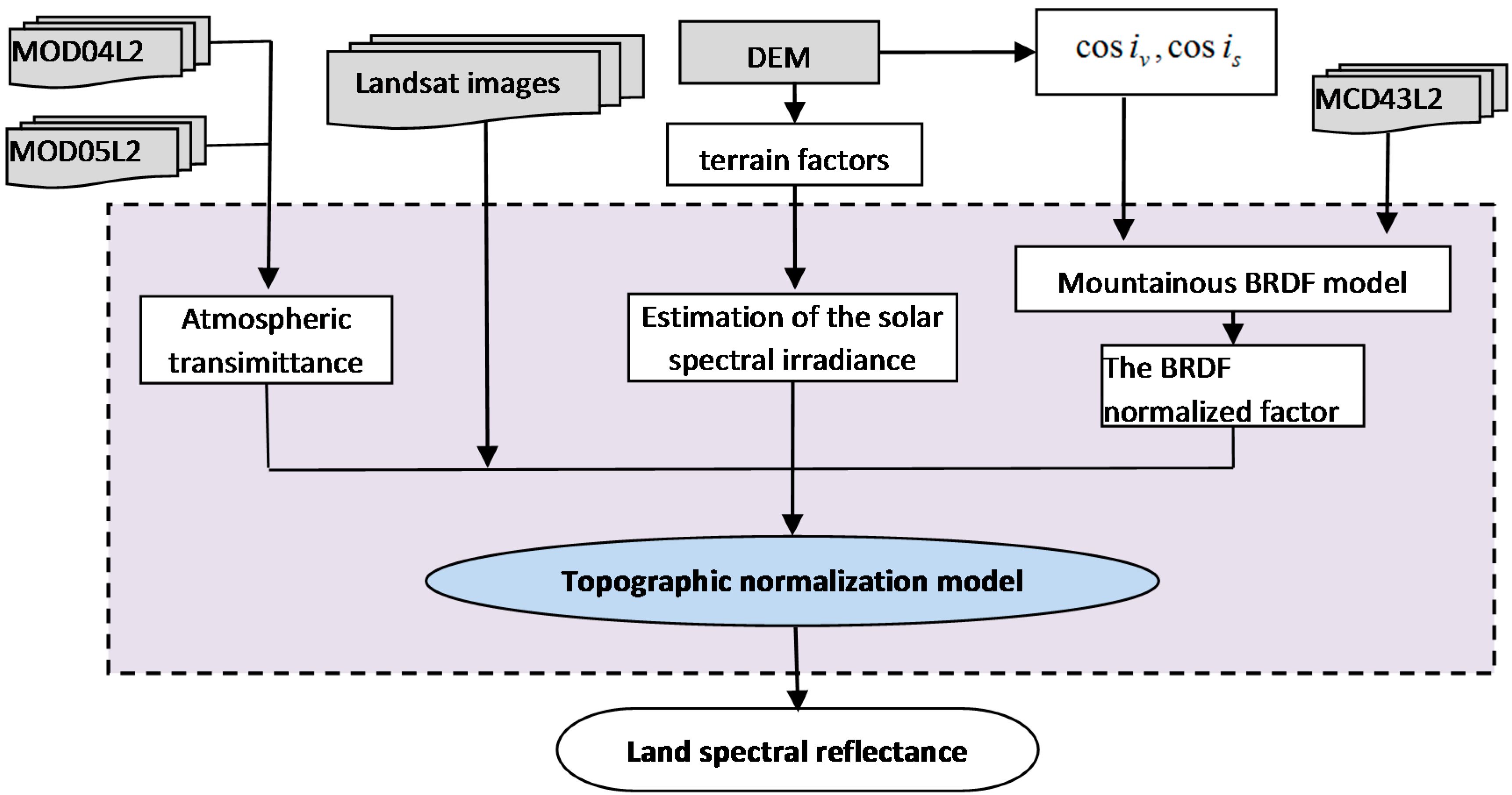
2.1. Improved Topographic Normalization

The TOA radiance L T O P ( λ ) (W∙m−2∙sr−1∙um−1) can be obtained through radiometric calibration according to the digital number (DN) values, offsets and gains provided by the image header files. This radiation computation consists of two parts, the path radiance L p ( λ ) and reflected radiance L ( λ ) from the land surface:
L T O P ( λ ) = L p ( λ ) + L ( λ ) T ( λ , θ v )       
where T ( λ,θ v ) is the atmospheric transmittance from the observing direction, which is a function of the sensor viewing angle, wavelength λ and atmospheric conditions [15]. The reflected radiance from the surface is determined by the surface reflectance in the space-based sensor observation direction and surface irradiance received from the sun. The global irradiance E ( λ )    can be decomposed into four components [34]. Therefore, the reflected radiance from the surface can be written as follows:
L ( λ ) = ( 1 / π ) ( E d i r ( λ ) + E a n i s o d i f ( λ ) ) ×     ρ T ( λ ) ( i s , i v , φ s v ) + ( 1 / π ) ( E i s o d i f ( λ ) + E r e f ( λ ) ) ρ T s d ( i v , φ v )   
Where E d i r ( λ ) , E i s o d i f ( λ ) , E a n i s o d i f ( λ ) and E r e f ( λ ) denote the direct, isotropic diffuse, anisotropic diffuse and surrounding-reflected spectral irradiance, respectively. ρ T ( λ ) is defined as the directional-directional reflectance caused by direct and anisotropic diffuse irradiance at the slope surface. ρ T s d ( λ ) is the hemispheric-directional reflectance caused by isotropic diffuse and surrounding-reflected irradiance [30]. In a slope and aspect ( S , A ) pixel, the zenith and azimuth angles in the directions of the solar incident and sensor observations are ( θ s , ϕ s ) and ( θ v , ϕ v ), respectively. However, because of topographic effects, the actual illumination angles between the solar beam and normal in a slope pixel will be modified as ( i s , ϕ s ) and ( i v , ϕ v ). ϕ s v is the relative azimuth between the sun and a satellite sensor, i.e., ϕ s v = | ϕ s ϕ v |      .
On an inclined surface, the local terrain can produce drastic variations in both the global irradiance and surface BRDF due to the changes in the associated angles, such as the actual zenith angle. Therefore, four actual angles on tiled surfaces must be changed in the new coordinate system based on the DEM, which can be calculated according to the literature [5]. Considering the small variation in the Landsat sensor view angle, the observed zenith and azimuth are assumed to be zero for each pixel [8]. The calculations for the actual observed zenith and azimuth angles on a given inclined surface can be simplified as:
cos i v = cos S
and
tan ϕ v = 0      
For the same land cover type, the inclined surface directional-directional reflectance ρ T ( λ ) ( i s , i v , φ s v ) can be differentiated from the flat surface directional-directional reflectance ρ H ( λ ) ( θ s , θ v , ϕ s v ) , which eliminates the topographic effects in mountainous areas. Both reflectances follow the BRDF characteristics, and their relationship can be expressed as
ρ T ( λ ) ( i s , i v , φ s v ) = Ω ( λ ) ( i s , i v , φ s v , θ s , θ v , ϕ s v ) × ρ H ( λ ) ( θ s , θ v , ϕ s v )   
where Ω ( λ ) ( i s , i v , φ s v , θ s , θ v , ϕ s v ) is defined as a BRDF normalized factor [1,30], which describes the transformation relation of the directional-directional reflectance transform caused by the topography.
In addition, because the hemispheric-directional reflectance is highly complex and the isotropic diffuse components and reflected irradiance are low on clear-sky days, the land surface can be reasonably assumed to obey isotropic characteristics. Therefore,
ρ T s d ( λ ) ( i v , φ v ) = ρ H ( λ ) ( θ s , θ v , ϕ s v )    
In Equation (1), the path radiance is generated by Rayleigh and aerosol scattering, and ρ r ( λ ) and ρ a ( λ ) denote Rayleigh and aerosol reflectances, respectively. The equation can then be expressed as
L P ( λ ) = D 0 E 0 ( λ ) cos θ s [ ρ r ( λ ) + ρ a ( λ ) ]    /π 
where D 0 is the calibration factor for the earth’s orbit, which is a deterministic parameter of sun-earth geometry; and E 0 ( λ ) (W∙m−2∙µm−1) is the extraterrestrial solar spectral irradiance at the time of the solar zenith angle θ s . A detailed description and discussion of Rayleigh and aerosol reflectances are provided in previous studies [15].
Combining Equations (2), (5) and (6) with Equation (1), the corrected reflectance is flat and completely free of topographic effects, rewritten as
ρ H ( λ ) ( θ s , θ v , ϕ s v ) = π ( L T O P ( λ ) L p ( λ ) ) / T ( λ , θ v ) [ ( E d i r ( λ ) + E a n i s o d i f ( λ ) ) Ω ( λ ) + ( E i s o d i f ( λ ) + E r e f ( λ ) ) ]    
When Ω ( λ ) = 1 , the surface is assumed to have Lambertian characteristics. Two cases are possible. The first case indicates that only the atmospheric effect is considered in the reflectance inversion from the images. Equation (8) is modified to the following form [35]:
ρ H ( λ ) ( θ s , θ v , ϕ s v ) = π( L T O P ( λ ) L p ( λ ) )   / T ( λ , θ v ) E 0 ( λ ) D 0 T ( λ , θ s )
The second case indicates that atmospheric and terrain effects influenced by the variation in the illumination angle are removed from the remote sensing images. In this case, the reflectance is estimated by [28]:
ρ H ( λ ) ( θ s , θ v , ϕ s v ) = π ( L T O P ( λ ) L p ( λ ) ) / T ( λ , θ v ) E ( λ )   
However, the value of the BRDF normalized factor is often not equal to 1 for the surface of anisotropic reflection characteristics in rugged terrain. Three important input parameters for inverting the sloping reflectivity are described in Section 3.

2.2. Comparison of Four Correction Algorithms

To validate the superiority of the improved topographic normalization, four additional algorithms were analyzed, as presented in Table 1. FLAASH is a MODTRAN-based atmospheric correction software package that provides accurate surface reflectances by estimating the amount of atmospheric water vapor and aerosols from the image directly [6]. The corresponding Landsat CDR [7] is the surface reflectance product distributed by USGS in the CDR.InEquation (9), the MODIS water vapor and aerosol products are input parameters for sole atmospheric correction, called the “MODIS-based atmospheric correction” (MBAC). Based on Equation (10), the method of topographic normalization by assuming a Lambertian surface is called the “MODIS-based Lambertian algorithm” (MBLA), and the atmospheric parameters are the same as those in MBAC. The topographic normalization proposed in this study is called the “MODIS-based BRDF algorithm” (MBBA), which is based on the MODIS BRDF/albedo kernel coefficient and MODIS atmospheric products.
Table 1. Basic descriptions of the four atmospheric and topographic normalization methods.
Method NameDEM and Terrain FactorsPWAOD
MODIS-based BRDF algorithm (MBBA)YESMOD05L2 MOD04L2
MODIS-basedLambertian algorithm (MBLA)YES MOD05L2MOD04L2
MODIS-based atmospheric correction (MBAC)NOMOD05L2 MOD04L2
Landsat climate data record (CDR)NO----
Fast line-of-sight atmospheric analysis of spectral hypercubes (FLAASH)NO -

3. Description of the Input Parameters

3.1. Atmospheric Transmittance

Atmospheric attenuation is caused by the interaction between solar radiation and the principal atmospheric constituents, which are highly sensitive to aerosol and water vapor concentrations, followed by Rayleigh scattering and the scattering and absorption by the ozone column. More detailed documentation can be found in the literature [36,37]. The atmospheric spectral transmittance formulas of the Landsat TM images follow Li’s model parameterization schemes [15].
T ( λ,θ s ) = T o 3 ( θ s ) T w ( θ s )    T r ( θ s ) T a ( θ s )
where T ( λ , θ s ) , T o 3 ( λ , θ s ) , T w ( λ,θ s ) , T r ( λ,θ s ) and T a ( λ,θ s ) denote the global spectral transmittance and component spectral transmittance caused by ozone and water vapor absorption, Rayleigh scattering and aerosol scattering.
Because of the relative stability over space and time, the correction of the atmospheric effects of ozone absorption and Rayleigh scattering is straightforward, as calculated by Li et al. [15]. However, in rugged terrain, the spatial distribution of aerosols and water vapor is highly variable over space and time for large regions, and their values are questionable if obtained by a semi-empirical formula or empirically at a single point. With the rapid development of the American NASA Earth Observing System Program (EOS), many remote sensors have provided abundant atmospheric products, such as the MODIS AOD and PW products, which have become reliable data sources for atmospheric parameters.
In this algorithm, the MODIS water vapor product PW (cm) can be directly input as the w parameter. The angstrom turbidity exponent α is provided by the MODIS AOD products. However, the β value is not directly available for MODIS AOD products and is in need of further deduction. The derivation method can be found in the literature [34]. The value of β can be expressed by
β = τ 0.55 ( 0.55 ) α   
where τ 0.55 is the AOD at a wavelength of 0.55µm, which is derived from the MODIS AOD products. Moreover, the local surface pressure can be estimated from the surface elevation [34].

3.2. Estimation of the Solar Spectral Irradiance

In mountainous areas, the global spectral irradiance can typically be decomposed into three components, i.e., direct, diffuse, and surrounding-reflected irradiances (Figure 2).Considering the direction of the sun, the diffuse irradiance is further divided into isotropic and anisotropic diffuse irradiances. All components are functions of the wavelength λ .The global irradiance can be expressed as follows [34]:
E ( λ ) = E d i r ( λ ) + E i s o d i f ( λ ) + E a n i s o d i f ( λ ) + E r e f ( λ )        
Figure 2. Solar irradiance on an inclined surface: (1) direct; (2) anisotropic diffuse; (3) isotropic diffuse; and (4) surrounding-reflected.
Remotesensing 07 06558 g002
Because of the variation in atmospheric conditions and terrain orientation, the spatial distribution of the irradiance components received on tiled surfaces presents strong spatial heterogeneity. Although the global irradiance and components are wavelength-dependent in Landsat images, formulas can follow the broadband estimation scheme described by Zhang et al. [34], except for the surrounding-reflected irradiance. The detailed calculation of the relevant terrain factors can be referenced in previous studies [26,15]. In addition, the TOA solar spectral irradiance of Landsat5 TM is replaced according to the official website [38].
The surrounding-reflected solar radiation can be estimated by
E r e f ( λ ) = π i = 1 n L i ( λ ) F i j         ( i = 1 , 2 , ... , n ) , i j   
where F i j is the topographic configuration factor, i.e., the ratio of the energy reaching the visible pixel to the energy emitted from the object pixel [15]. L i ( λ ) is the surface-reflected radiance measured via a satellite.

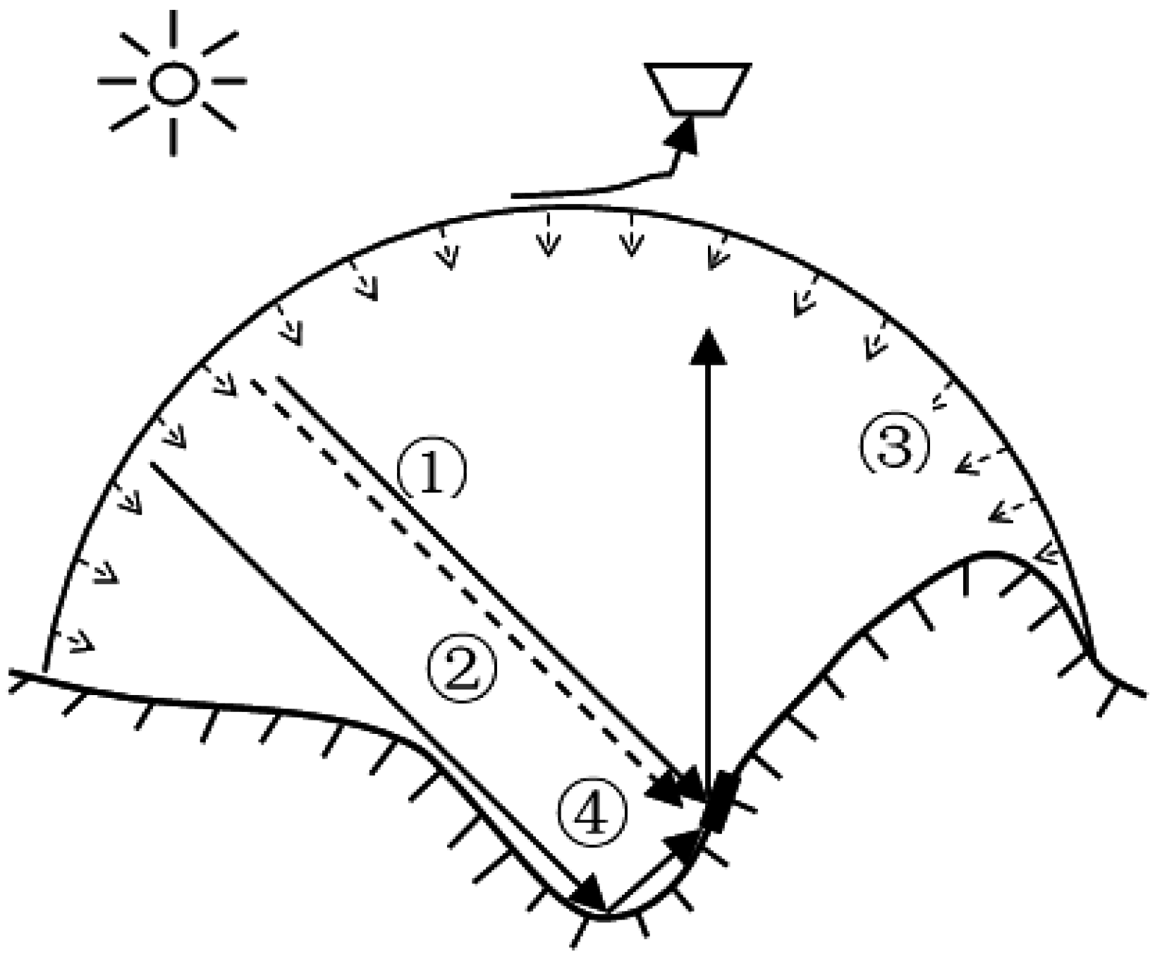
3.3. Bidirectional Reflectance Distribution Function (BRDF) Model

The BRDF normalized factor Ω ( λ ) ( i s , i v , φ s v , θ s , θ v , ϕ s v ) is defined as the ratio of the tilted surface reflectance to the flat surface reflectance [1,30], eliminating the influence of terrain on homogenous land cover. Two types of reflectivity are all directional-directional reflectance, which obey BRDF laws. The BRDF considers surface reflectance properties at a particular wavelength to be a function of the angle of incidence and observation angles, which can correct directional anisotropy caused by shadows, buildings or topography [39]. The MODIS BRDF/Albedo model parameter product (MCD43A1) was derived based on a 16-day reflectance dataset from MODIS on Terra and Aqua using the kernel-driven semi-empirical Ambrals BRDF model. This model can be used to calculate the directional reflectance at any desired viewing and solar geometries. The quality is assessed using the MCD43A2 QA (Quality Assessment) layer, which shows that the quality declines sequentially when the quality flags vary from 0 to 4.
Mathematically, the Ross Thick-Li Sparse kernel-driven BRDF model is a linear combination of isotropic (defined as a constant value of 1) volume and geometric optical scattering kernels, which are given by Schaaf et al. [31].
ρ H ( λ ) ( θ s , θ v , ϕ s v ) = f i s o ( λ ) + f v o l ( λ ) K v o l ( θ s , θ v , ϕ s v ) + f v o l ( λ ) K g e o ( θ s , θ v , f s v )
where K v o l ( θ s , θ v , ϕ s v ) and K g e o ( θ s , θ v , ϕ s v )    are kernel functions that depend only on the viewing and illumination geometries. The detailed algorithm of the two kernel functions can be found in Schaaf et al. [31]. f i s o ( λ ) , f v o l and f v o l are the BRDF model empirical parameters provided directly by the MODIS BRDF product to describe the weights of the three kernel functions, i.e., the isotropic, volume and geometric optical scattering parameters, respectively. However, the spatial resolution of the MODIS BRDF parameter C005 is 500 m, which cannot be directly applied to the 30 m TM images. The parameters require downscaling to 30 m according to the land classification maps. According to the land cover types of the Landsat imagery, the BRDF parameters for each class at the MODIS scale are extracted. Based on land-type-specific BRDF correction factors, which hypothesize that the reflectances should be similar at the Landsat and MODIS spatial resolutions, the 30 m scale of the BRDF parameters for each pixel is extracted. Further details of the methodology can be found in the literature [40]. However, the average effect of the BRDF parameters using a 500 m MODIS BRDF to correct 30 m Landsat imagery was not addressed here.
Generally, the geometric relationship of the sun-surface-sensor is fixed on a flat surface at a given local time; thus, the two kernel functions are constant values. The MODIS BRDF/Albedo product does not explicitly consider slope and aspect effects [12]. However, the two kernel functions will change for each pixel in rugged terrain due to the intensive variation in the actual illumination and sensor observation angles with the surface slope and aspect. In areas with significant slopes, the BRDF is no longer symmetric about the principal plane, and it must be corrected by adding the aspect and slope from a DEM [31]. Therefore, considering the slope and aspect variations, the slope reflectivity can be calculated by
ρ T ( λ ) ( i s , i v , φ s v ) = f i s o ( λ ) + f v o l ( λ ) K v o l ( i s , i v , φ s v ) + f g e o ( λ ) K g e o ( i s , i v , φ s v )    

4. Results and Validation

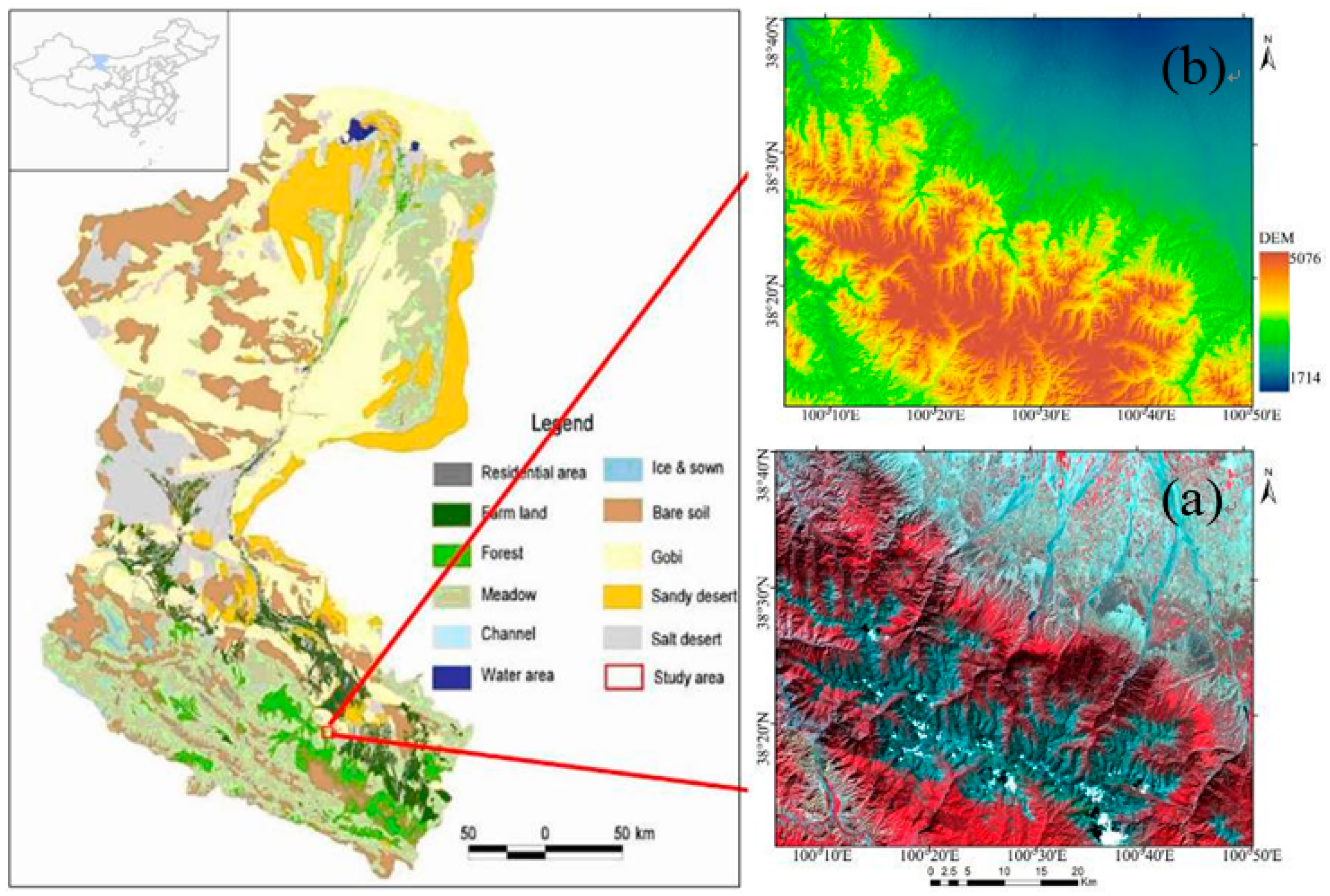
4.1. Study Area and Data

The selected study area is located in the upper stream of the Heihe River Basin, a typical inland river basin in Northwest China [41], as shown in Figure 3. The area has hilly terrain and an altitude between 1714 m and 5076 m above sea level. There are five types of land cover in the area: farmland, forest dominated by Picea crassifolia, grass, water bodies and bare surface [42,43]. Furthermore, the land cover is largely distributed according to terrain characteristics, particularly the terrain aspect caused by the solar radiation heterogeneity. The forest primarily covers the north-facing slope, farmland and grass cover the flat or gentle south-facing slopes, and bare land is widely distributed on the steep southern slope [34].
Figure 3. Details of the study area based on a (a) DEM and (b) false-color composite (RGB: band 4, 3 and 2).
Remotesensing 07 06558 g003
The dataset for this study consists of a GDEM (30 m) derived from ASTER [44], MODIS PW and AOD atmospheric products (MOD05_L2 and MOD04_L2) with spatial resolutions of 1 km × 1 km and 10 km × 10 km (at nadir), respectively, the MODIS BRDF/Albedo product (MCD43A1) and a Landsat TM image (WRS path/row of 133/033, Level 1T product) acquired on August 11, 2009, at a solar zenith of 31.82° and a solar azimuth of 131.26°. In addition, a corresponding Landsat CDR [7] was applied for validating the atmospheric correction and topographic normalization. These data were obtained from the USGS Earth Resources Observation System (EROS) Data Center and were projected to Universal Transverse Mercator (UTM) coordinates.

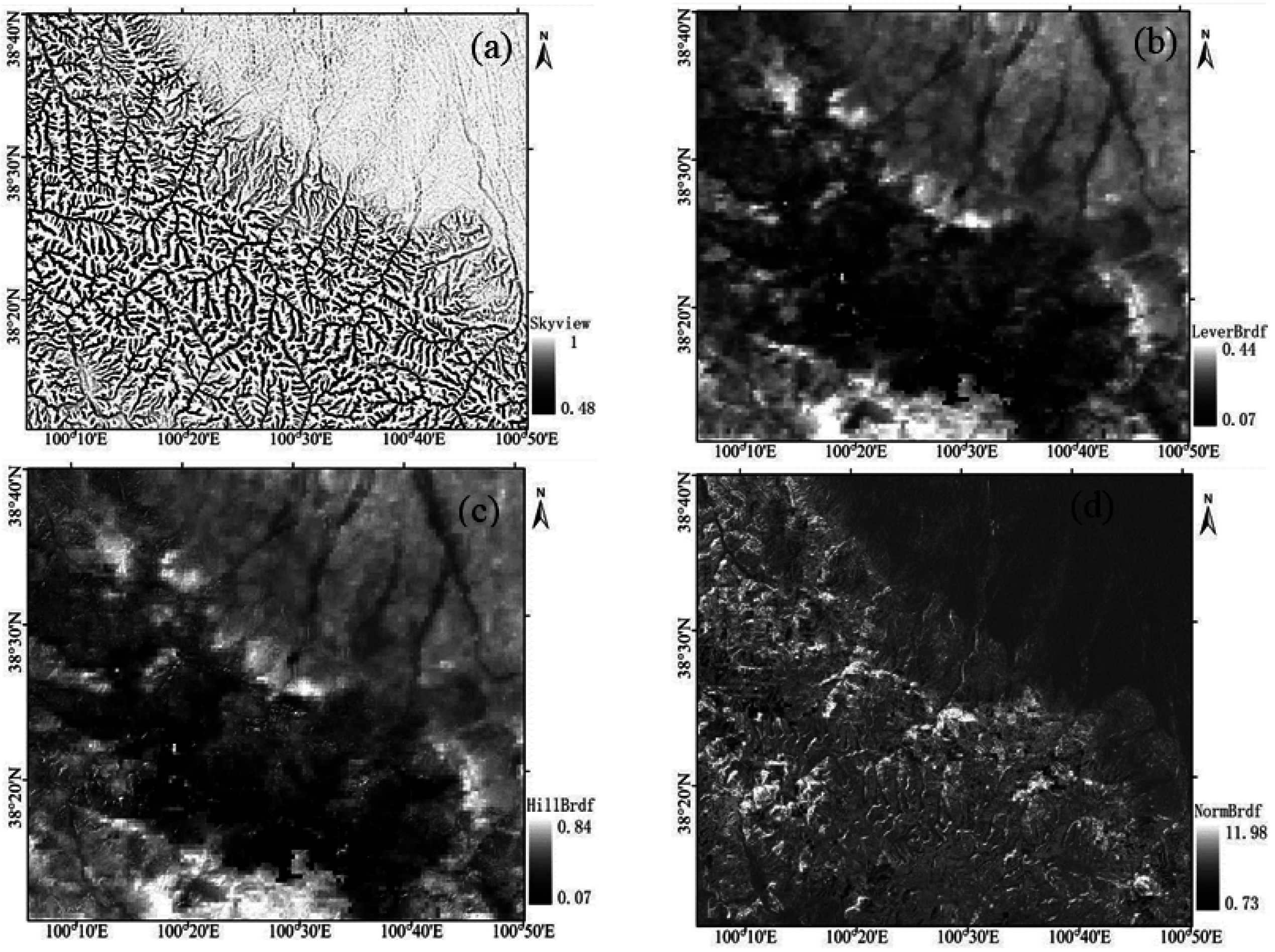
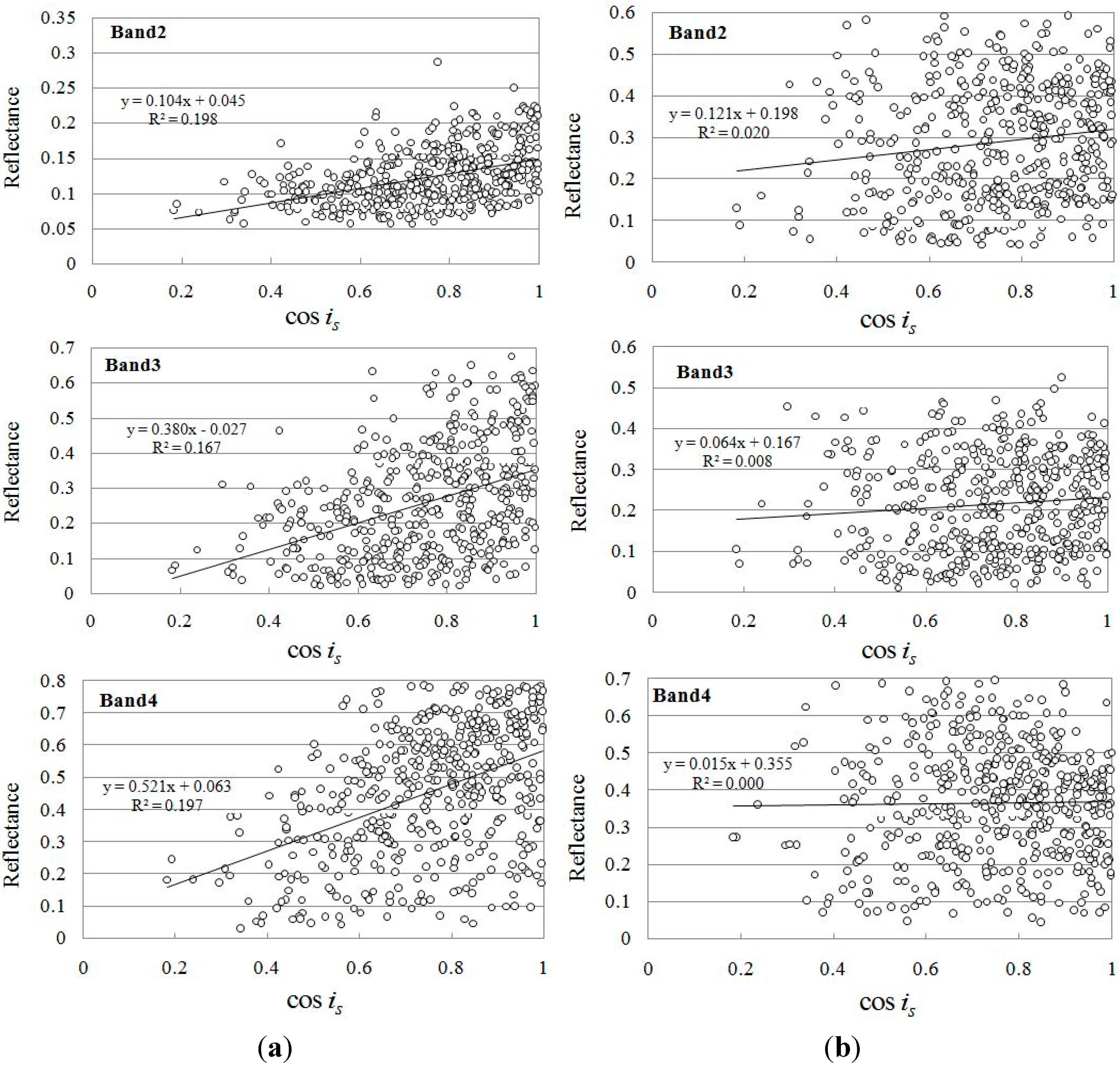
4.2. Bidirectional Reflectance Distribution Function (BRDF) Normalized Factor

Using high-resolution DEM data, important topographic factors, such as the slope, aspect, obstruction coefficient, and sky view factor, are obtained for each pixel with sloping terrain. The flat surface directional reflectivity (LevelBrdf) and corresponding tilted pixel directional reflectivity (HillBrdf) can be derived using an Ambrals forward model based on the MODIS BRDF/Albedo parameter product. In this manner, the BRDF normalized factor (NormBrdf) is obtained; Figure 4 shows the spatial distributions in band 4.
Figure 4. Sky view factor, bidirectional reflectance distribution function (BRDF) of sloping and flat pixels, and BRDF normalized factor: (a) sky view factor; (b) Level BRDF; (c) Hill BRDF; and (d) Norm BRDF.
Remotesensing 07 06558 g004

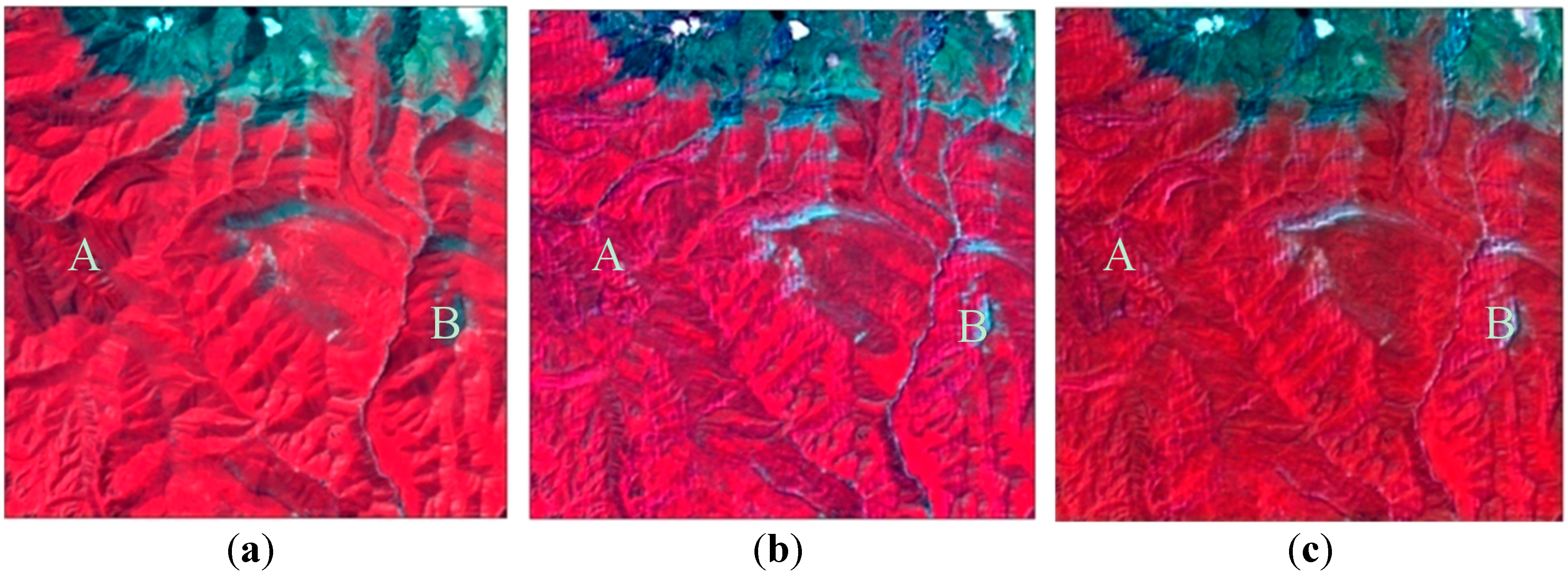
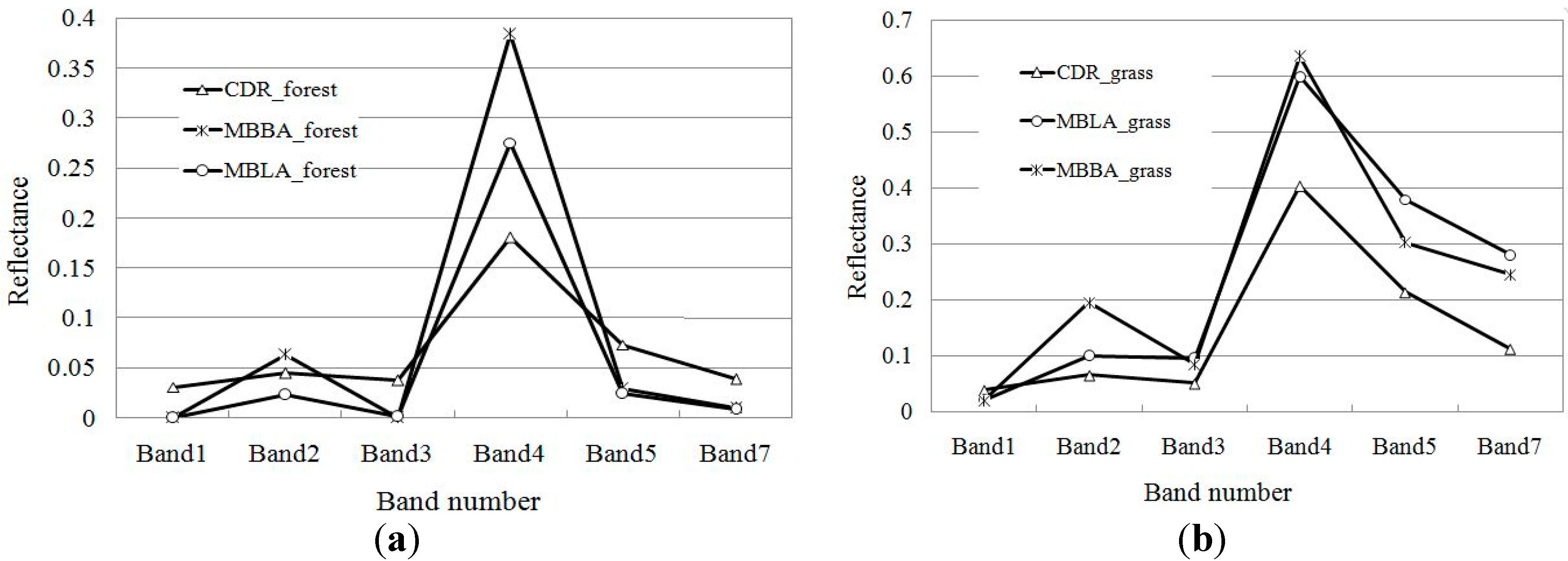
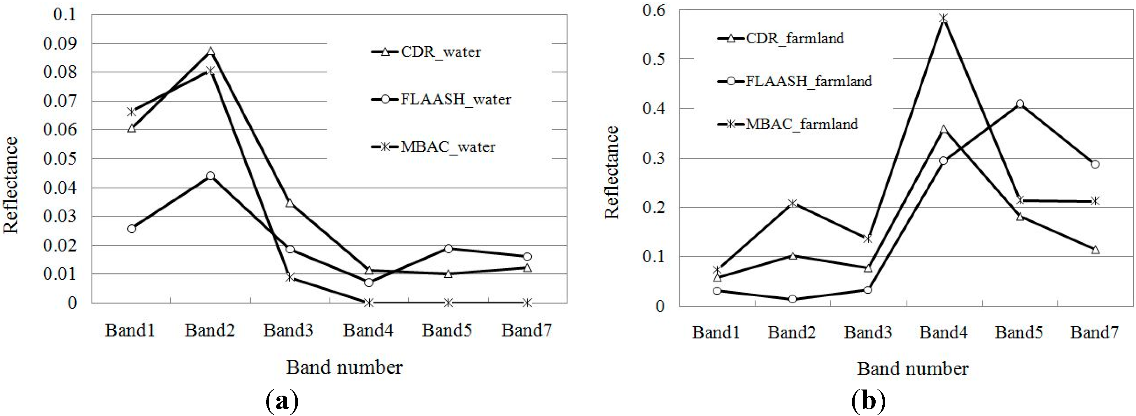
4.3. Validation and Discussion

To achieve topographic normalization, the sloping reflectance derived from the sensor must be converted to a flat reflectance based on atmospheric and topographic correction, as expressed in Equation (8).There are two main methods for validating the merit of the topographic correction: visual inspection and quantitative accuracy analysis. Figure 5 shows the result of the partially enlarged images for a clear visual interpretation of the topographic normalization. The corresponding reflectance composite images of bands 4 (red), 3 (green), and 2 (blue) are also shown in Figure 5b. There were terrain effects in the original imagery of the rugged area, as seen by the dark shadows and bright regions facing the sun. The MBBA and MBLA can eliminate or at least reduce the terrain influence and flatten surfaces compared with the raw images (Figure 5a). Two topographic normalization methods can improve the pixel reflectance of self-shadowing and shadowing areas and reduce the contrast of surface features on shady and sunny slopes. After removing the terrain effects, more detailed features can emerge and improve the amount of information available in images. However, the MBLA overcorrects the reflectance in deep shady locations, such as areas A and B, by assuming isotropic surface reflectance. In contrast, the MBBA can reduce the overcorrection effects by considering the surface BRDF (Figure 5c).Moreover, both the MBLA and MBBA methods generate artifacts over bright areas within the image, possibly because the solar radiation was underestimated due to the AOD and PW overestimation of the MODIS atmospheric products [34].
Figure 5. False-color composite (RGB: bands 4, 3, and 2) of the original images and after the topographic normalization: (a) the original images; (b) MODIS-based Lambertian algorithm (MBLA); and (c) MODIS-based BRDF algorithm (MBBA).
Remotesensing 07 06558 g005
True surface measurements of these spectra are lacking. Moreover, in cold and arid study regions, terrain characteristics determine the spatial distribution of land cover types. It is very difficult to sample suitable areas with uniform vegetation on the sunny and shady sides of hills. Thus, in this test region, unsupervised or supervised classification on the original and corrected images is not feasible for accuracy evaluation. Therefore, other quantitative evaluation methods must be applied.
In general, testing whether the cosine of the solar illumination angle and the surface reflectance are linearly correlated has become a quantitative analysis method to verify the topographic normalization. Therefore, 481 pixels were randomly selected for the quantitative analysis in different terrain conditions and land cover types. Figure 6a shows that the reflectance of the sole atmospheric correction varies with the terrain and the cosine of the illumination angle in bands 2, 3, and 4, which are significantly positively correlated with the cosine of the illumination angle. However, the linear relationships between the pixel reflectance and cosine of the incident angle are eliminated or significantly weakened after considering the terrain effects in the same bands (Figure 6b).
In addition, the spectral curves of the four typical features are extracted to verify the advantage of this method insole atmospheric correction and topographic normalization. First, in flat areas, two types of surfaces are selected to illustrate the effectiveness of the atmospheric correction method, MBAC, MODIS atmospheric products as input parameters. As shown in Figure 7, the MBAC can effectively remove the influence of water vapor and aerosols and restore the true spectra of both water and farmland compared with FLAASH and Landsat CDR. Second, Figure 8a indicates that the spectrum of a shady forest pixel (the northwest-facing slope of 34) was enhanced overall in the MBAC compared with the MBLA and Landsat CDR. The spectrum of a relatively flat grass pixel (the southwest-facing slope of 15) was also restored. Moreover, the reflectance of shady forests was further increased after the terrain correction, and the degree of improvement was larger when considering the surface BRDF, particularly in band 4 (Figure 8a).
Figure 6. Scatterplot of the cosine of the illumination angle vs. the pixel reflectances in bands 2, 3, and 4: (a) sole atmospheric correction (MBAC) and (b) terrain normalization (MBBA).
Remotesensing 07 06558 g006
Figure 7. The spectra of the MBAC compared with the FLAASH and Landsat CDR in flat areas: (a) water pixel; and (b) farmland pixel.
Remotesensing 07 06558 g007
Figure 8. The spectra of the MBBA compared with the MBLA and Landsat CDR: (a) forest pixel (northwest-facing slope); and (b) grass pixel (southwest-facing slope).
Remotesensing 07 06558 g008
High relief can lead to topography-related image distortion, whereas the topographic slope and aspect can influence the natural spectral variability. Based on the above comparative analysis, surface features distorted by atmospheric and topographic effects can be realistically reproduced using this algorithm.

5. Conclusions and Discussion

This study presents a method for topographic normalization with two novel features. First, the BRDF normalized factor is used to convert a sloping pixel reflectance into a flat pixel reflectance. Second, MODIS aerosol and water vapor products are directly used as input parameters to determine the atmospheric attenuation.
However, a careful analysis of Figure 5c shows that the topographic effects are not completely eliminated. In areas of broken terrain, the “topography” still exists on images corrected topographically, and overcorrection and even some noise is still present in low illumination areas. These overcorrection or residual topographic effects are related to several factors. First, the estimation of global solar irradiance is inaccurate in the low-illumination region, which is underestimated or overestimated. The direct solar radiation is relatively simple, but the estimation of diffuse and surrounding-reflected radiation has larger uncertainties. Second, the MODIS water vapor and aerosol products are considered sources of significant error because of the product inversion algorithms [34,45]. Third, a DEM spatial resolution of 30 m is not sufficient for TM images for topographic normalization [28]. Because the DEMs determine the pixel elevation and crucial terrain factors and ultimately affect the quality of the topographic normalization, the DEM grid size should be smaller than the scale of the original image. However, in addition to data acquisition difficulties, utilizing high-resolution DEMs to obtain the target pixel more accurately than topographic factors at the sub-pixel scale has been difficult; this is important to address in future research. Finally, the information gap caused by temporal and spatial resolutions between the MODIS products and the Landsat imagery is ignored in the current work, possibly leading to discrepancies in the scale of the BRDF parameters, atmospheric conditions, and illumination conditions. Furthermore, for imagery in different seasons, the solar zenith angle should be standardized to reduce the remaining BRDF effect caused by variations in the sun angle [1].

Acknowledgments

The work was supported by the NSFC project–(Grant No.91225302), the Chinese Academy of Sciences Action Plan for West Development Program Project (Grant No. KZCX2-XB3-15), and the National Science Foundation of China (Grant No.41061038). The data used in the paper were obtained from the Watershed Allied Telemetry Experimental Research.

Author Contributions

Yanli Zhang and Xin Li designed the research and formulated the model. Jianguang Wen helped construct the model. Qinhuo Liu and Guangjian Yan significantly contributed to the manuscript’s revision. Yanli Zhang analyzed the data and wrote the paper. All of the authors contributed to the discussion of the results.

Abbreviation

DSSR
downward surface shortwave radiation (W∙m−2)
AOD
aerosol optical depth
PW
precipitable water (cm)
BRDF
surface bidirectional reflectance distribution function
DEM
digital elevation model
TOA
top of the atmosphere
L T O P ( λ )
at-satellite radiance
L p ( λ )
path radiance
L ( λ )
reflected radiance from the land surface
T ( λ , θ v )
atmospheric transmittance from the observing direction
E 0 ( λ )
extraterrestrial solar spectral irradiance (W∙m−2∙µm−1)
E ( λ )
global spectral irradiance (W∙m−2∙µm−1)
E d i r ( λ )
direct spectral irradiance (W∙m−2∙µm−1)
E i s o d i f ( λ )
isotropic diffuse spectral irradiance (W∙m−2∙µm−1)
E a n i s o d i f ( λ )
anisotropic isotropic diffuse spectral irradiance (W∙m−2∙µm−1)
E r e f ( λ )
surrounding-reflected spectral irradiance (W∙m−2∙µm−1)
E d i f h o r ( λ )
diffuse spectral irradiance on the horizontal surface
ρ T ( λ )
directional-directional reflectance
ρ T s d ( λ )
hemispheric-directional reflectance
S , A
slope and aspect
θ s , φ s
zenith and azimuth angles in the directions of solar incident
θ v , φ v
zenith and azimuth angles in the directions of sensor observations
i s , ϕ s
actual zenith and azimuth angles in the directions of solar incident due to topographic effects
i v , ϕ v
actual zenith and azimuth angles in the directions of sensor observations due to topographic effects
ρ T ( λ ) ( i s , i v , ϕ s v )
inclined surface directional-directional reflectance
ρ H ( λ ) ( θ s , θ v , φ s v )
flat surface directional-directional reflectance
Ω ( λ ) ( i s , i v , ϕ s v , θ s , θ v , φ s v )
BRDF normalized factor
D 0
calibration factor for the Sun-Earth distance
θ s
solar zenith angle
cos i s
cosine of the solar illumination angle of a sloping grid
V s
obstruction coefficient
T ( λ , θ s )
global spectral transmittance
T o 3 ( λ , θ s )
spectral transmittance caused by ozone
T w ( λ , θ s )
spectral transmittance caused by water vapor absorption
T r ( λ , θ s )
spectral transmittance caused by Rayleigh scattering
T a ( λ , θ s )
spectral transmittance caused by aerosol scattering
V i s o
sky view factor
F i j
topographic configuration factor
K
circumsolar view factor or anisotropy index
L i ( λ )
surface-reflected radiance measured via a satellite

Conflicts of Interest

The authors declare no conflicts of interest.

References

  1. Flood, N.; Danaher, T.; Gill, T.; Gillingham, S. An operational scheme for deriving standardised surface reflectance from Landsat TM/ETM+ and SPOT HRG imagery for Eastern Australia. Remote Sens. 2013, 5, 83–109. [Google Scholar] [CrossRef]
  2. Flood, N. Testing the local applicability of MODIS BRDF parameters for correcting Landsat TM imagery. Remote Sens. Lett. 2013, 4, 793–802. [Google Scholar] [CrossRef]
  3. Kobayashi, S.; Sanga-Ngoie, K. A comparative study of radiometric correctionmethods for optical remote sensing imagery: the IRC vs. other image-based Ccorrection methods. Int. J. Remote Sens. 2009, 30, 285–314. [Google Scholar] [CrossRef]
  4. Liang, S.; Fang, H.; Chen, M. Atmospheric correction of Landsat ETM+ land surface imagery. I. Methods. IEEE Trans. Geosci. Remote Sens. 2001, 39, 2490–2498. [Google Scholar] [CrossRef]
  5. Li, F.; Jupp, D.L.; Reddy, S.; Lymburner, L.; Mueller, N.; Tan, P. A physics-based atmospheric and BRDF correction for Landsat data over mountainous terrain. Remote Sens. Environ. 2012, 124, 756–770. [Google Scholar] [CrossRef]
  6. Kruse, F.A. Comparison of ATREM, ACORN, and FLAASH atmospheric corrections using low-altitude AVIRIS data of Boulder, CO. In Proceedings of the 13th JPL Airborne Geoscience Workshop, Pasadena, CA, USA, 31 March–2 April 2004.
  7. Masek, J.G.; Vermote, E.F.; Saleous, N.E.; Wolfe, R.; Hall, F.G.; Huemmrich, K.F.; Gao, F.; Kutler, J.; Lim, T.K. A Landsat surface reflectance dataset for North America, 1990–2000. IEEE Geosci. Remote Sens. Lett. 2006, 3, 68–72. [Google Scholar] [CrossRef]
  8. Li, F.; Jupp, D.L.B.; Reddy, S.; Lymburner, L.; Mueller, N.; Tan, P.; Islam, A. An evaluation of the use of atmospheric and BRDF correction to standardize Landsat data. IEEE J. Sel. Top. Appl. Earth Observ. Remote Sens. 2010, 3, 257–270. [Google Scholar] [CrossRef]
  9. Liang, S.; Fang, H.; Chen, M.; Shuey, C.J. Validating MODIS land surface reflectance and albedo products: Methods and preliminary results. Remote Sens. Environ. 2002, 83, 149–162. [Google Scholar] [CrossRef]
  10. Pons, X.; Pesquer, L.; Cristóbal, J.; González-Guerrero, O. Automatic and improved radiometric correction of Landsat imagery using reference values from MODIS surface reflectance images. Int. J. Appl. Earth Observ. Geoinf. 2014, 33, 243–254. [Google Scholar] [CrossRef]
  11. Román, M.O.; Gatebe, C.K.; Schaaf, C.B.; Poudyal, R.; Wang, Z.; King, M.D. Variability in surface BRDF at different spatial scales (30m–500m) over a mixed agricultural landscape as retrieved from airborne and satellite spectral measurements. Remote Sens. Environ. 2011, 115, 2184–2203. [Google Scholar] [CrossRef]
  12. Roy, D.P.; Ju, J.; Lewis, P.; Schaaf, C.; Gao, F.; Hansen, M.; Lindquist, E. Multi-temporal MODIS—Landsat data fusion for relative radiometric normalization, gap filling, and prediction of Landsat data. Remote Sens. Environ. 2008, 112, 3112–3130. [Google Scholar] [CrossRef]
  13. Balthazar, V.; Vanacker, V.; Lambin, E.F. Evaluation and parameterization of ATCOR3 topographic correction method for forest cover mapping in mountain areas. Int. J. Appl. Earth Observ. Geoinf. 2012, 18, 436–450. [Google Scholar] [CrossRef]
  14. Kobayashi, S.; Sanga-Ngoie, K. The integrated radiometric correction of optical remote sensing imageries. Int. J. Remote Sens. 2008, 29, 5957–5984. [Google Scholar] [CrossRef]
  15. Li, X.; Koike, T.; Cheng, G.D. Retrieval of snow reflectance from Landsat data in rugged terrain. Ann. Glaciol. 2002, 34, 31–37. [Google Scholar]
  16. Hantson, S.; Chuvieco, E. Evaluation of different topographic correction methods for Landsat imagery. Int. J. Appl. Earth Observ. Geoinf. 2011, 13, 691–700. [Google Scholar] [CrossRef]
  17. Richter, R.; Kellenberger, T.; Kaufmann, H. Comparison of topographic correction methods. Remote Sens. 2009, 1, 184–196. [Google Scholar] [CrossRef] [Green Version]
  18. Vanonckelen, S.; Lhermitte, S.; van Rompaey, A. The effect of atmospheric and topographic correction methods on land cover classification accuracy. Int. J. Appl. Earth Observ. Geoinf. 2013, 24, 9–21. [Google Scholar] [CrossRef]
  19. Vanonckelen, S.; Lhermitte, S.; van Rompaey, A. The effect of atmospheric and topographic correction on pixel-based image composites: Improved forest cover detection in mountain environments. Int. J. Appl. Earth Observ. Geoinf. 2015, 35, 320–328. [Google Scholar] [CrossRef]
  20. Richter, R. Correction of atmospheric and topographic effects for high spatial resolution satellite imagery. Int. J. Remote Sens. 1997, 18, 1099–1111. [Google Scholar] [CrossRef]
  21. Cebecauer, T.; Suri, M.; Gueymard, C. Uncertainty sources in satellite-derived direct normal irradiance: How can prediction accuracy be improved globally. In Proceedings of the SolarPACES Conference, Granada, Spain, 20–23 September 2011.
  22. Dozier, J.; Frew, J. Rapid calculation of terrain parameters for radiation modeling from digital elevation dat. IEEE Trans. Geosci. Remote Sens. 1990, 28, 963–969. [Google Scholar] [CrossRef]
  23. Hay, J.E.; McKay, D.C. Estimating solar irradiance on inclined surfaces: A review and assessment of methodologies. Int. J. Solar Energy 1985, 3, 203–240. [Google Scholar] [CrossRef]
  24. Proy, C.; Tanre, D.; Deschamps, P.Y. Evaluation of topographic effects in remotely sensed data. Remote Sens. Environ. 1989, 30, 21–32. [Google Scholar] [CrossRef]
  25. Sandmeier, S.; Itten, K.I. A physically-based model to correct atmospheric and illumination effects in optical satellite data of rugged terrain. IEEE Trans. Geosci. Remote Sens. 1997, 35, 708–717. [Google Scholar] [CrossRef]
  26. Li, X.; Cheng, G.; Chen, X.; Lu, L. Modification of solar radiation model over rugged terrain. Chin. Sci. Bull. 1999, 44, 1345–1349. [Google Scholar] [CrossRef]
  27. Richter, R. Correction of satellite imagery over mountainous terrain. Appl. Opt. 1998, 37, 4004–4015. [Google Scholar] [CrossRef] [PubMed]
  28. Zhang, Y.L.; Yan, G.J.; Bai, Y.L. Sensitivity of topographic correction to the DEM spatial scale, IEEE Geoscience and Remote Sensing Letters. Geosci. Remote Sens. Lett. 2015, 12, 53–57. [Google Scholar] [CrossRef]
  29. Shepherd, J.D.; Dymond, J.R. Correcting satellite imagery for the variance of reflectance and illumination with topography. Int. J. Remote Sens. 2003, 24, 3503–3514. [Google Scholar] [CrossRef]
  30. Wen, J.G.; Liu, Q.H.; Xiao, Q.; Liu, Q.; Li, X.W. Modeling the land surface reflectance for optical remote sensing data in rugged terrain. Sci. China Ser. D-earth Sci. 2008, 51, 1169–1178. [Google Scholar] [CrossRef]
  31. Schaaf, C.B.; Li, X.; Strahler, A.H. Topographic effects on bidirectional and hemispherical reflectances calculated with a geometric-optical canopy model. IEEE Trans. Geosci. Remote Sens. 1994, 32, 1186–1193. [Google Scholar] [CrossRef]
  32. Gao, B.; Jia, L.; Menenti, M. An improved method for retrieving land surface albedo over rugged terrain. IEEE Geosci. Remote Sens. Lett. 2014, 11, 554–558. [Google Scholar] [CrossRef]
  33. Wen, J.; Zhao, X.; Liu, Q.; Tang, Y.; Dou, B. An improved land-surface albedo algorithm with DEM in rugged terrain. Geosci. Remote Sens. Lett. 2014, 11, 883–887. [Google Scholar]
  34. Zhang, Y.L.; Li, X.; Bai, Y.L. An integrated approach to estimate shortwave solar radiation on clear-sky days in rugged terrain using MODIS atmospheric products. Solar Energy 2015, 113, 347–357. [Google Scholar] [CrossRef]
  35. Chander, G.; Markham, B. Revised Landsat-5 TM radiometric calibration procedures and postcalibration dynamic ranges. IEEE Trans. Geosci. Remote Sens. 2003, 41, 2674–2677. [Google Scholar] [CrossRef]
  36. Leckner, B. The spectral distribution of solar radiation at the earth’s surface—Elements of a model. Solar Energy 1978, 20, 143–150. [Google Scholar] [CrossRef]
  37. Yang, K.; Koike, T.; Ye, B. Improving estimation of hourly, daily, and monthly solar radiation by importing global data sets. Agric. For. Meteorol. 2006, 137, 43–55. [Google Scholar] [CrossRef]
  38. Landsat 5 (L5) Thematic Mapper (TM). Available online: http://landsat.usgs.gov/science_L5_cpf.php (accessed on 19 May 2015).
  39. Wanner, W.; Strahler, A.H.; Hu, B.; Lewis, P.; Muller, J.P.; Li, X.; Barnsley, M.J. Global retrieval of bidirectional reflectance and albedo over land from EOS MODIS and MISR data: Theory and algorithm. J. Geophys. Res. Atmosp. 1997, 102, 17143–17161. [Google Scholar] [CrossRef]
  40. Shuai, Y.; Masek, J.G.; Gao, F.; Schaaf, C.B. An algorithm for the retrieval of 30-m snow-free albedo from Landsat surface reflectance and MODIS BRDF. Remote Sens. Environ. 2011, 115, 2204–2216. [Google Scholar] [CrossRef]
  41. Li, X.; Li, X.W.; Li, Z.; Ma, M.; Wang, J.; Xiao, Q.; Liu, Q.; Che, T.; Chen, E.; Chen, G.; et al. Watershed allied telemetry experimental research. J. Geophys. Res. 2009, 114. [Google Scholar] [CrossRef]
  42. Zhang, Y.L.; Li, X. Topographic normalization of landsat TM images in rugged terrain based on the high-resolution DEM derived from ASTER. In Proceedings of the PIERS Proceeding, Suzhou, China, 12–16 September 2011; pp. 712–716.
  43. Zhang, Y.L.; Li, C.R.; Wang, X.Q.; Zhang, P.J. Preparation of high-resolution DEM in Dayekou Basin based on the WorldView-2 and its accuracy analysis. Remote Sens. Technol. Appl. 2013, 28, 431–436. [Google Scholar]
  44. Using ASTER and SRTM DEMs for Studying Geomorphology and Glaciation in High Mountain Areas. Available online: http://www.earsel.org/symposia/2004-symposium-Dubrovnik/pdf/150.pdf (accessed on 19 May 2015).
  45. Zhou, C.Y.; Liu, Q.H.; Tang, Y.; Wang, K.; Sun, L.; He, Y.X. Comparison between MODIS aerosol product C004 and C005 and evaluation of their applicability in the north of China. J. Remote Sens. 2009, 13, 854–872. [Google Scholar]

