1. Introduction
Hyperspectral remote sensing (HRS) is a common tool for environmental and geoscience applications [
1]. Enabled by high spatial, spectral and temporal resolutions—together with broad coverage and a high level of accuracy—
airborne HRS image data has proved especially useful and continues to pose new possibilities for quantitative surface recognition and classification within these fields. In the last decade, many HRS sensors have become commercially available to the field of remote sensing [
1], and many users are now being exposed to this promising technology.
The key factor in extracting quantitative information from HRS images in all configurations (single or multi-sensor) is radiometric accuracy. Accurate at-sensor radiometric information is essential to retrieving realistic reflectance values. The ground reflectance retrieved from the at-sensor radiance is commonly used for qualitative and quantitative surface mapping. Extraction of reliable reflectance values from at-sensor radiance requires radiative transfer correction using physical atmospheric models. For this purpose, both accurate radiometric data and atmospheric correction are important.
In this regard, a leading project to improve satellite platforms is the Quality Assurance Framework for Earth Observation QA4EO [
2]. Based on a set of “inter-operable” guidelines, the QA4EO has provided a framework for the intergovernmental Group on Earth Observations (GEO) to establish a representative, unequivocal and universal quality indicator (QI). The QA4EO advises on how to run similar comparisons for earth observation measurements—whether between sensors or between ground measurement devices.
The main aim of is to found regulations, standards and product validation on inter-calibrated data, as revealed in the ESA DUE GlobColour project (GC-RS-UOP-SAR-01). Ground based campaigns are an important instrument to perform accurate sensor calibration and inter-calibration. For this purpose several CalVal diagnostic sites are proposed, there access to information, including textural and spectral information, is shared on a project basis through dedicated portals. These sites have to be spectrally featureless, stable and homogeneous, easy to maintain and access, and well documented.
The EO data originating from selected space-borne systems (MERIS, AATSR, ALOS AVNIR2 and ALOS PRISM) are systematically acquired over those internationally agreed diagnostic sites, which include the EOS Land core sites and the Ocean diagnostic sites as well as ALOS Calibration Team defined sites. The dataset of characteristic geophysical properties is accessible from the internet, a powerful search interface allows dedicated data queries.
The CEOS Land Product Validation (LPV) group is to coordinate the quantitative validation of satellite-derived products. Furthermore, the European commissioned, “EUFAR FP7—JRA2: HYQUAPRO”, is an ongoing initiative that provides quality layers for airborne hyperspectral imagery and data products via end-to-end processing chain with harmonized quality measures [
3,
4,
5]. The initiative is also active in promoting additional projects to improve airborne HRS imagery data.
Successful use of information on a given area from several hyperspectral sensors relies on the ability to extract realistic, rather than apparent, reflectance. As each sensor might perform differently, a crucial stage is calibrating each sensor to the quality level that will provide reliable data. This is especially important when performing data analyses based on different sensors or even with the same sensor on different dates. An example of this is discussed in [
6], where spectral change detection for a HyMAP sensor over the same area a year apart showed that sensor-performance instability introduces uncertainty in the results.
As noted, the quality of the atmospheric-correction procedure relies on the quality of the radiometric data. All non-orbital sensors undergo routine laboratory calibration on a yearly basis, but they might deteriorate between calibration periods. Moreover, cross-correlation between the multiple sensors in a multi-sensor mission is important but apparently not always performed. As a result, the quality of the reflectance results acquired simultaneously by multiple sensors might vary with each independent sensor’s radiometric quality. A cross-calibration site along with a method to inspect and, if necessary, correct the radiometric laboratory-calibrated data for each individual sensor are crucial stages in the full data-processing chain.
Vicarious calibration (VC) sites and methods have been proposed as a solution to the aforementioned problems. Most of these methods estimate radiometric and atmospheric calibration coefficients by repeatedly solving the radiative transfer response using ground-truth information measured during (or close in time to) the sensor overpass. The acquired at-sensor radiance is iteratively compared with the modeled radiance and an objective function or recalibration coefficients are generated. The iteration is successfully completed when the at-sensor radiance adjusts to the modeled radiance. An alternative approach is a look-up table (LUT) that first uses the ground-truth radiance to pre-compute a database of spectra representing radiometric quantities and atmospheric properties based on a range of input parameters (such as in-flight calibration of the ATCOR model) with numerous forward atmospheric simulations (MODTRAN). This physically based modeling procedure relies on an absolute radiometric calibration and effective spectral-matching format. The traditional VC relies on the empirical line (EL) assumption [
7,
8,
9] that ground targets should be spectrally known and stable, affected as little as possible by the atmosphere, and located near the area of interest (AOI), covering a large area and range of albedos [
9,
10,
11,
12]. They also have to be spectrally featureless, isotropic, stable and homogeneous, easy to access and maintain, and well documented for every mission.
Alternative methods for in-flight calibration of satellite sensors have long been developed and proposed. A regionally specific vicarious calibration study for the Sea-Viewing Wide-Field-of-View Sensor (SeaWiFS) and Moderate Resolution Imaging Spectroradiometer (MODIS) sensors was suggested and discussed [
13]. The system vicarious calibration for the Visible Infrared Imaging Radiometer Suite (VIIRS) sensor has been analyzed based on the normalized water-leaving radiance data collected at the WaveCIS AERONET-OC site of Gulf of Mexico [
14]. A radiative transfer (RT) based vicarious approach for satellite sensors which makes use of high quality data from multiple existing (worldwide of the ocean color component) sites has been recently suggested [
15].
Meeting the above requirements for HRS sensors is seldom, if ever, possible for every mission of orbital sensors in general, and airborne sensors in particular. As these requirements are difficult to fulfill, Brook
et al. [
16] suggested applying a supervised VC (SVC) approach in which a selected bright site is manipulated to satisfy them. The main assumption of the SVC method is that radiometric and spectral performance and stability of all HRS sensors vary in time and space, and therefore the periodical calibration information, such as laboratory calibration, might not be correct or suitable for a particular campaign. However, as it is crucial that sensors remain radiometrically and spectrally calibrated in order to achieve synergy and multi-sensor data fusion, the SVC method is suggested to maintain the overall accuracy and stability of the at-sensor radiance response, as well as correct possible radiance drift.
The SVC approach has been studied in several flight campaigns using a single airborne HRS sensor (AisaDUAL in Israeli national campaigns, HyMap in FP7 EO-miners Sokolov campaign). The innovative SVC approach, however, has not yet been used for multi-sensor campaigns or in respect to conditions (of geography, illumination, flight direction or landscape) that vary between campaigns in which data are acquired simultaneously. The present study was thus aimed to apply a cross-calibration SVC method and examine the resultant image quality by using quality assurance (QA) and quality indicators (QIs) based on the ground SVC site and the net targets. The preliminary results were previously reported and discussed [
17]. We therefore organized and conducted a challenging campaign utilizing three airborne HRS sensors under the EUFAR Transnational Access (TA) program in a project entitled ValCalHyp. The sensors were: AisaDUAL on board the DORNIER 288 (operated by NERC), and AHS and CASI-1500i on board the CASA C-212 (operated by INTA). The study areas were located in the south of France. The SVC site was located near Montpellier and the thematic areas were Salon-de-Provence, Marseille, Avignon and Montpellier. The mission took place on 28 October 2010 between 12:00 and 16:00 UTC.
The paper unfolds as follows: the methodology and a brief overview of the sensors used for the cross-calibration mission and the SVC test site are discussed in
Section 2. The results and the validation measures are reported in
Section 3.
Section 4 consists of a discussion of the results and conclusions.
2. Methodology
In practice, the SVC method relies on in-situ spectral measurements of a specific selected test site situated along the airplane’s trajectory. The site is a wide spanning, homogeneously bright surface that is covered by artificial agriculture nets (black polyethylene nets) of various densities. The varying net density against the same bright background enables the establishment of a linear sequence of shadings that cover the HRS sensor’s dynamic range. Moreover, if the bright target has any particular absorption feature, the radiometric sequence between this natural target and the different net densities might model and even prevent possible negative effects, such as artifacts, during subsequent processing stages. In general, the nets can be assembled (rolled out) at the site (near the airfield) just before the overpass and should be measured for radiance at the time of the overpass, regardless of platform altitude. Because reflectance of isotropic targets (like the suggested calibration nets) is a time-independent parameter, it can therefore be measured at any time. The net targets have been found to hold important information on the quality of the data and can lead to accurate data correction.
The proposed approach does not require iterations other than those inherent in the SVC optimization and calibration-processing stages (e.g., F1 in
Figure 1) as described in [
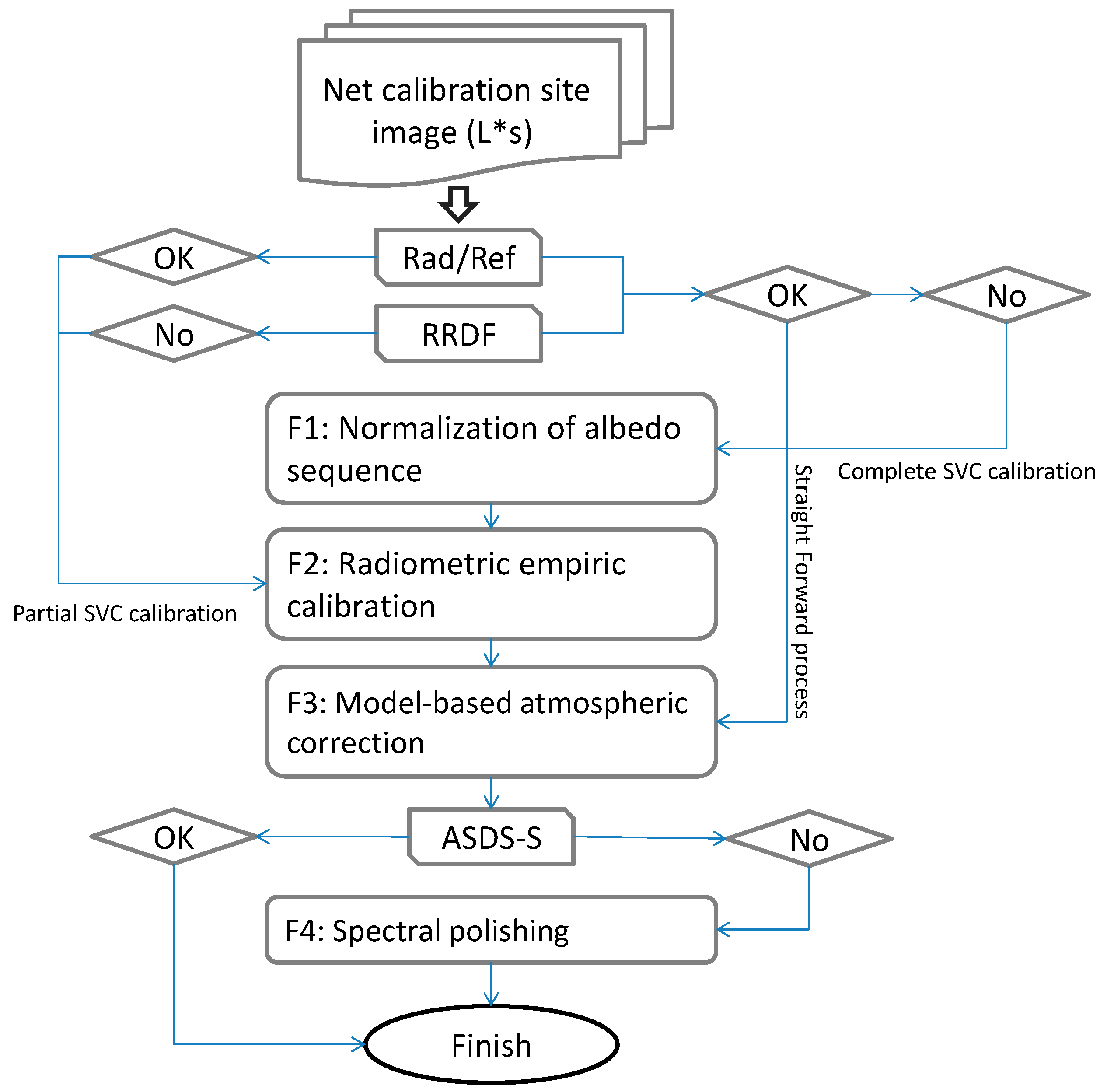
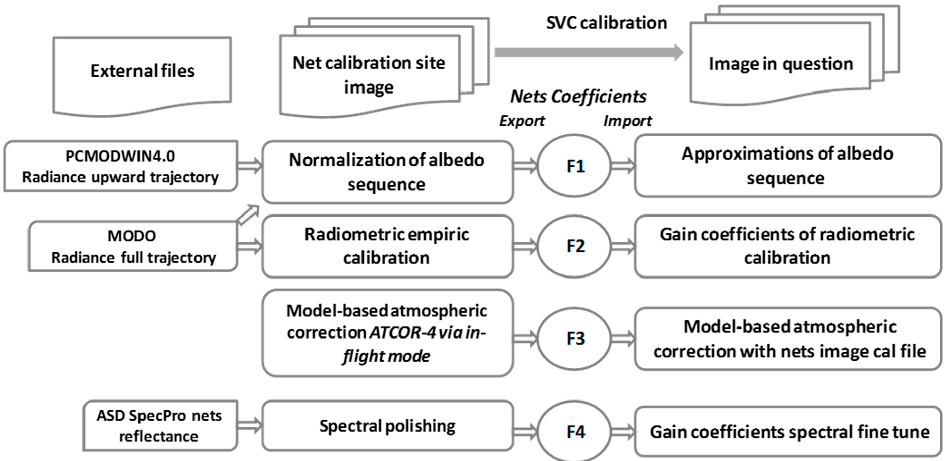
16]. In general, the SVC correction is based on four stages (
Figure 1): inspection of the data followed by normalization of the albedo sequence of the sensor’s radiance (F1), radiometric calibration using the net reflectance to obtain L(gain) (F2), model-based atmospheric correction (F3), and spectral polishing using the net reflectance (F4). The generated calibration factors were applied to all mission scenes and the thematic maps were created.
Figure 1.
The complete SVC calibration scheme [
16].
Figure 1.
The complete SVC calibration scheme [
16].
Critical to multi-source data integration is the radiometric concurrence of each individual sensor. Numerous techniques for calibration and validation require in-situ or model-based predictive parameters. The proposed method suggests utilization of both in-situ and model-based radiance. This approach is sufficient for analyzing both absolute and relative radiometric accuracy and thus allows cross-comparison and data integration between data sets acquired by multiple airborne sensors, even if the data acquisitions do not overlap in time.
2.1. Data Acquisition
First, a brief overview of the sensors used for cross-calibration is provided. The AisaDUAL is a pushbroom airborne imaging spectrometer designed and built by Specim Ltd (Oulu, Finland,
http://www.specim.fi). This system was operated by NERC (UK) on board a DORNIER 228 aircraft at an altitude of 3.3 km. The acquired imagery data in this campaign consists of 286 pixels in the cross-track direction and hundreds of pixels in the along-track direction. It provides a pixel size of 1.6 m
2 for simultaneously acquired images in varying configurations of contiguous spectral bands. In the ValCalHyp mission, this sensor was configured to 190 bands between 400 and 970 nm [visible near infrared (VNIR) region] and 244 bands between 970 and 2450 nm (shortwave infrared (SWIR) region). It is composed of two sensors: AisaEAGLE for the VNIR region and AisaHAWK for the SWIR region. A standard AisaDUAL dataset is a 3D non-geo-rectified data cube. The geo-correction and rectification are performed based on INS–GPS data.
The AHS sensor is a whiskbroom airborne imaging spectrometer with 80 bands which is designed, manufactured and built by Sensytech Inc. (currently Argon ST, and formerly Daedalus Inc. (PA, USA,
http://www.daed.com), and is owned and operated by INTA (ES) since 2003. This system was operated by the INTA (ES) team on board a CASA C-212 aircraft at an altitude of 2.1 km. The acquired imagery data in this campaign consists of 750 pixels in the cross-track direction and hundreds of pixels in the along-track direction. This sensor is configured to 19 bands with widths of approximately 19 nm between 400 and 1000 nm (VNIR region), 3 bands at 1001 nm, 1589 nm and 1920 nm, 41 continuous and fairly narrow bands with a width of approximately 13 nm between 2010 and 2500 nm, and 17 relatively wide spectral bands (30–50 nm) across the mid and long thermal wavelengths covering both atmospheric windows between 3 and 5 µm and 8 and 13 µm respectively. The obtained pixel size for the current sensor configuration was 5.8 m
2.
The CASI-1500i sensor is a pushbroom airborne VNIR imaging spectrometer designed and built by Itres Ltd (AB, Canada,
http://www.itres.com). This system was operated by the INTA (ES) team on board the CASA C-212 together with the AHS system at an altitude of 2.1 km. The acquired imagery data in this campaign consists of 1500 pixels in the cross-track direction and hundreds of pixels in the along-track direction, enabling imaging of a vast area with a single pass. It simultaneously acquires images in varying configurations of contiguous spectral bands (144 bands in this mission) covering the 380–1050 nm spectral region with spatial resolution of 1.13 m
2.
2.2. Ground Sites of Interest
The ground SVC site was set up two hours prior to the flight campaign near Montpellier (
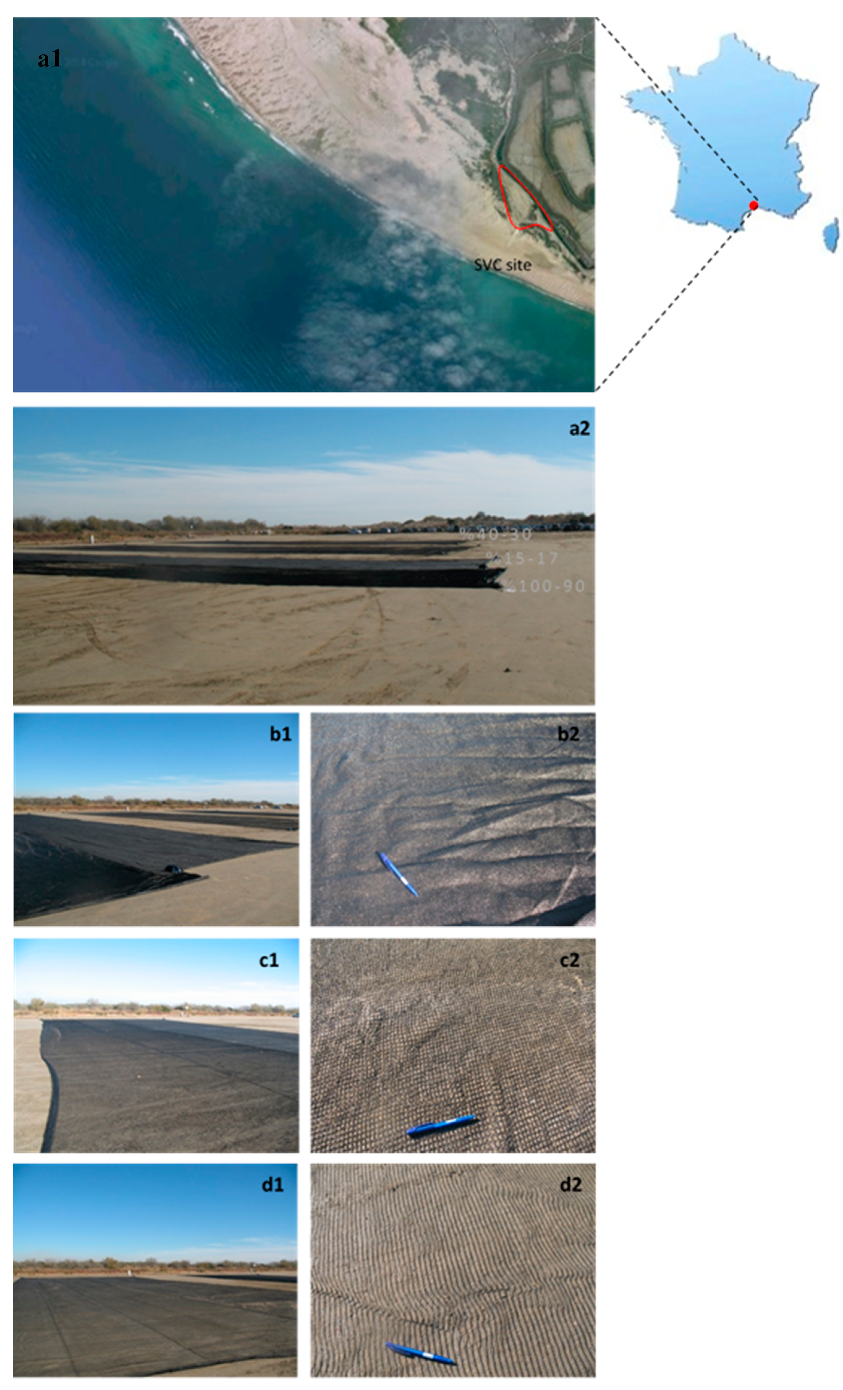
Figure 2) on quartz dune sand serving, which serves as a parking area near the coastline. This site provided a spacious flat region covered mainly with very bright sand. The size of each net was 50 × 20 m, and each section was classified as: “darkest and most dense” (90%–100% net cover); “middle density” (30%–40% net cover); or “brightest and least dense” (17%–15% net cover).
The ground spectra of the SVC targets were measured with a portable field spectrometer (ASD SpecPro; Analytical Spectral Devices, Boulder, CO, USA) consisting of 2151 wavelengths ranging between 350 and 2500 nm, with band widths of 2 nm in the VNIR region (350–1050 nm) and 10 nm in the SWIR region (1050–2500 nm), and a wavelength accuracy of ±1 nm/±0.1 nm. Each ground target (the nets, the background surface and the additional validation targets) was measured by averaging 40 spectra of both radiance and reflectance values just before and during the overpass. The reflectance mode was calculated as a ratio against a Spectralon® white reference panel. The optimization procedure was programmed to work in both radiance and reflectance modes, averaging 40 replications per measured spectrum. Each target was measured systematically by collecting about 40 points along the net area. The nadir measurements, which maintained the same position relative to the sun, and all points in a designed matrix were about 3 m distant from each other and the spectral measurement was taken from 1 m height with a bare-optics with 24° field of view (about 60 cm2 footprint) with a spectral error (standard deviation) of between 0.1% and 1.0% (standard spectral error) expected for Spectralon®. All spectra were averaged to yield a single mean corrected spectrum for each of the net targets (in both reflectance and radiance units), which were later resampled to the sensor’s spectral configuration (band spectral wavelength and band width).
Figure 2.
Landsat 8 image (a1), SVC site marked in red (43.48°N, 4.14°E GCS WGS84) near Montpellier, France (source—google,imagery@2014 data SOI, NOAA, U.S.) and ground digital photo of SVC site (a2). Net targets are labeled as follows: (b1) is the darkest and most dense net (90%–100% net cover) and (b2) is a zoom-in image (respective scale is a standard pen); (c1) is the middle density net (30%–40% net cover) and (c2) is a zoom-in image, and (d1) is the brightest and least dense net (17%–15% net cover) and (d2) is a zoom-in image.
A main concern in many studies [
18,
19] is the bidirectional reflectance distribution factor (BRDF), which is significant at the image edges. In this project, we followed [
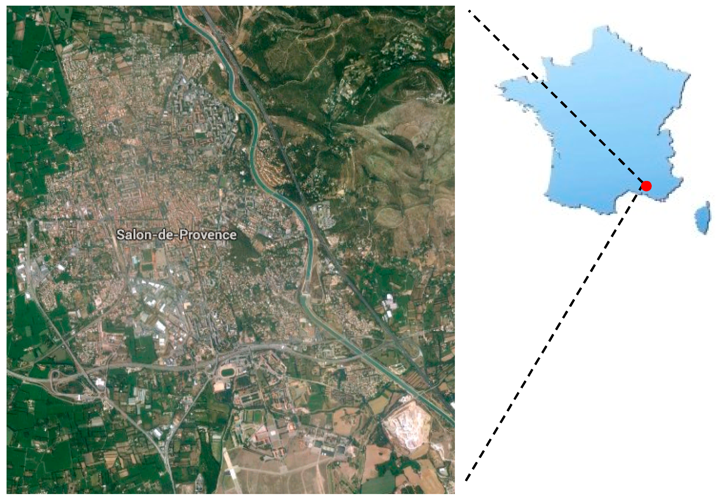
16] suggestion and located the SVC site in the center of the HRS flight lines’ images, collecting many ground-truth spectra using the described measurement protocol. As previously mentioned, two thematic area sites were acquired during this campaign in the south of France. The first area was an urban region in Salon-de-Provence (
Figure 3) and the second was a maritime region in the port of Marseille (
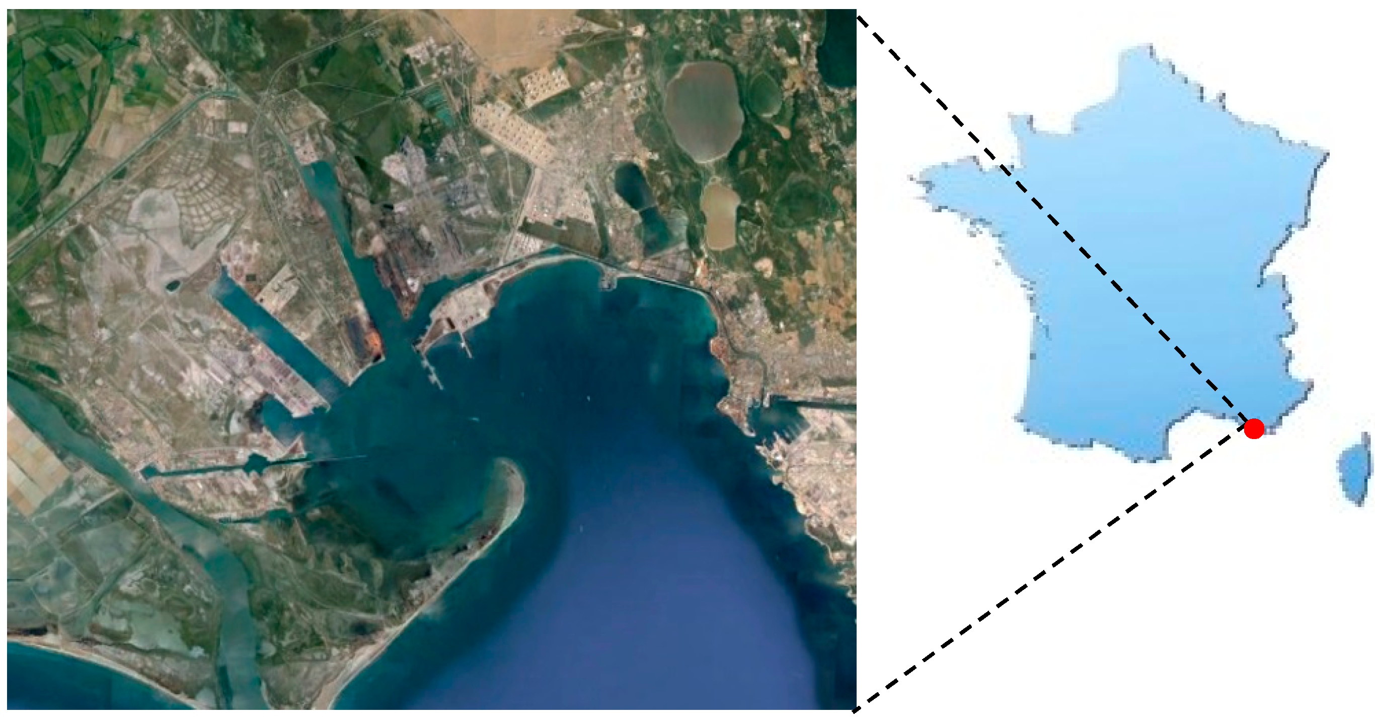
Figure 4).
Figure 3.
Validation site—urban region in Salon-de-Provence (43.64°N, 5.09°E GCS WGS84), France (source—google, imagery@2014 data SOI, NOAA, U.S.).
Figure 3.
Validation site—urban region in Salon-de-Provence (43.64°N, 5.09°E GCS WGS84), France (source—google, imagery@2014 data SOI, NOAA, U.S.).
Figure 4.
Validation site—maritime region near the port of Marseille (43.41°N, 4.87°E GCS WGS84), France (source—google, imagery@2014 data SOI, NOAA, U.S.).
Figure 4.
Validation site—maritime region near the port of Marseille (43.41°N, 4.87°E GCS WGS84), France (source—google, imagery@2014 data SOI, NOAA, U.S.).
2.3. SVC Cross-Calibration Method and Correction Stages
The airborne at-sensor HRS radiance data were subjected to preprocessing stages prior to their radiometric inspection and correction: vertical stripes were removed using the destriping algorithm [
20]; noise across 1400 nm and 1800 nm spectral regions known as water vapor absorption and spectral saturation were spatially masked out; and the boresight effect was estimated for the AisaDUAL image data [
16]. The airborne L1 imagery data were radiometrically corrected in digital number (DN) format by the data suppliers (INTA ES, [
21]; NERC UK, [
22]) using empirical line function for laboratory-base gain and offset coefficients and providing the at-sensor radiance imagery.
2.3.1. Radiometric Quality Indicators
The overall sensitivity assessment of the entire sensor–atmosphere–surface interface system is highly important for further data-processing stages. A well-known image-based measure is the environmental noise equivalent radiance difference (NEΔL
s) proposed by [
23] and further implemented by [
24]. This ratio parameter is dependent on the instrument’s signal-to-noise ratio (SNR)—with marked influences of noise in the image data (e.g., adjacency and shadow effects)—and is calculated from the at-sensor radiance image [
23]. Since this method could not indicate the radiometric performance, the accuracy levels, or radiometric deviation or uncertainty due to the flight heading or BRDF impact, alternative methods were proposed and developed (e.g., [
16]).
The radiance quality was inspected using the QIs Rad/Ref (the at-sensor radiance-to-reflectance ratio) and RRDF (radiance-to-reflectance difference factor) indicators as suggested by [
16]. According to calibration theory, the ground-truth measured radiance equals the sun’s radiance above the atmosphere at a nadir–zenith angle times the atmospheric transmittance coefficient, adding the selective scattering contribution (Rayleigh and Mie) to the sensor output. Assuming that the HRS sensor holds the calibration coefficients generated in the laboratory, the at-sensor radiance is aligned accordingly. Systematic drift from the laboratory calibration is not considered; therefore, high radiometric accuracy is not obtained and the data hinder precise model-based atmospheric correction.
Several known or unknown factors encountered during sensor transport, installation and/or even data acquisition might destabilize the radiometric performance. Indeed, the achieved at-sensor radiance is a product of the “real” or true radiance multiplied by L(gain) and adding L(offset) coefficients that adjust the information to the at-sensor radiance, particularly for miss-calibrated laboratory coefficients.
Prior to extracting the abovementioned coefficients, it is important to inspect and validate the radiance performance using QIs for each sensor separately. The most common radiometric investigation uses MODTRAN (PCMODWIN4.0) to reconstruct the atmosphere above the sensed surface and then compares the results with the obtained at-sensor radiance [
19]. This requires access to an atmospheric model (or any radiative transfer code) and continuous running of the code until full parameterization that produces solid answers is obtained. Alternatively, the at-sensor radiance (Ls) can be examined by its corresponding reflectance without applying any radiative model [
16] using the Rad/Ref and RRDF indicators.
The first QI, Rad/Ref, is developed according to Equations (1) and (2), where the at-sensor radiance (Ls) is divided by the surface reflectance coefficient (ρ) of a selected ground target (e.g., SVC nets).
where Εο is the sun’s radiance above the atmosphere at a certain zenith angle, τ is the atmospheric transmittance, ρ is the reflectance spectrum and L(path) is the selective scattering contribution (Rayleigh and Mie). The L(gain) and L(offset) parameters bias the acquired at sensor radiance from real radiance.
If the sensor is well-calibrated, (1) the at-sensor radiance (Ls) represents the real radiance (L(gain) = 1 and L(offset) = 0); and (2) Rad/Ref stays constant if no path radiation occurs (Equation (3)).
If L(path) = 0, then the at-sensor radiance-to-reflectance ratio Ls/ρ(Rad/Ref) should be constant at any wavelength, as all terms in τΕο/π are constant for nearby targets. Assume that above 800 nm, L(path) = 0; then for all ground targets (regardless of their reflectance), the Rad/Ref spectra must give a similar response under any acquisition condition. In the SWIR region, the Rad/Ref value should be equal for all (net) targets (L(path) = 0), and across the VNIR region (L(path) > 0), the Rad/Ref value must hold a sequence presented by the L(path)/ρ term. This term is inversely proportional to the reflectance values of the calibration targets: as L(path) is constant for all of the net targets, Rad/Ref holds opposite reflectance sequences. Note, however, that we need to ensure that the targets selected for this examination are located close to each other to maintain identical values of L(path) and τ across the 400–800 nm (visible; VIS) region. If L(gain) ≠ 1 and L(offset) ≠ 0, as occurs with noncalibrated sensors, Ls/ρ produces variation curves above 800 nm with no opposite albedo sequence in the VNIR region. These factors are easy to assess and can shed light on the quality of the data prior to any serious investigation or further processing steps (e.g., atmospheric calibration stage). The Rad/Ref indicator is a quantitative regulator for inspection of the data quality and the radiometric performance of the sensor in question. The second factor for assessing the quality of the radiometric output uses the set of net measurements and calculates the radiance-to-reflectance difference ratio (Equation (4)) termed RRDF.
where 1 and 2 refer to any pair of examined nets (e.g., net 1: 17% and net 2: 90% cover percentages).
The RRDF (constant response) obtained in Equation (4) is invariant with respect to the surface reflectance. Therefore, all calculated RRDF responses should be identical (assuming stable and constant atmosphere above the SVC site at the time of the overpass).
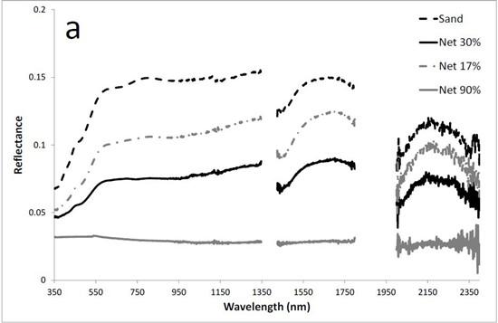
Performance of the suggested QIs can be examined by comparing the optimal indicators (as generated from theoretical radiance and measured reflectance) of the SVC targets to the actual image radiance and measured reflectance. Both parameters are examined against a theoretical full-trajectory at-sensor-level radiance (Rad; PCMODWIN 4.0 RT (radiative transfer) code) simulated based on ground-reflectance measurements (ASD SpecPro).
The Rad/Ref indicator should be examined for each spectral region independently (VIS, NIR and SWIR). In the VIS region, we suggest using the peak band of the maximum Rad/Ref curve inspecting the albedo sequence. In the SWIR region, any band, aside from water-vapor-attenuation wavelengths, can be selected (as the response of all bands should be equal).
2.3.2. Radiometric Correction Using the SVC Ground Site
For each SVC target, a theoretical indicator (calculated for the same solar and atmospheric conditions applying PCMODWIN 4.0 RT radiative transfer code for the ground-truth spectra) is plotted against the actual value and a correlation between the theoretical or modelled (Rad/Ref) indicator (at three selected wavelengths across the VIS, NIR and SWIR regions) and the nets' known densities is plotted. Then a 95% confidence interval is set defining the range of the actual image indicator values examined. The actual image indicator values are examined by applying Levene’s test (
F-test), which simply calculates the position of the actual image (spectral) indicator and its equality within the accepted confidence interval of the optimal indicator (a significance level > 0.05 means that the results are indistinct and are therefore rejected; a significance level < 0.05 means the results are significant and accepted at 95% confidence). The Student’s
t-test significance level is used to examine the single value indicator: at a significance level > 0.05, the results are indistinct and rejected; at a significance level between 0.01 and 0.05, the results are significant at 95% confidence and are accepted, and at a significance level < 0.01, the results are significant at 99% confidence and are accepted. The final stage is correlation and distribution examination between actual image indicator values and the 95% confidence interval of the optimal indicators using the Pearson R coefficient (Equation (5)):
where x and y are deviation scores (normalized by the mean score of each variable).
The means of the deviation scores are both 0; if not, there is no relationship between x and y. reveals the relationship between x and y as well. If there is no relationship, then positive values of x are just as likely to be paired with negative values of y as with positive values of y. This makes negative values of xy as likely as positive values and the is small. If there is a positive or negative relationship, then the is high. The rules for the examination and the decision-making process are determined further on.
The RRDF indicator inspects the entire spectral region. The theoretical indicators retrieve equal values for all net targets; therefore, the examination of actual image variables is based on the same decision-making process as the Rad/Ref indicator.
The two suggested parameters, Rad/Ref and RRDF, and their statistics (versus theoretical values) which are simply derived from the calibration net targets, can immediately spot faulty performance of the sensor prior to subsequent data-processing stages (correction via L(gain) and L(offset) or atmospheric correction via models). If for any reason, the sensor is not performing well, the estimation of L(gain) and L(offset) is performed by VC as will be discussed in
Subsection 2.3.3).
2.3.3. The SVC Correction Stages
The Rad/Ref and RRDF indicators were examined for each HRS image individually and, where necessary, L(gain) and L(offset) coefficients were evaluated using the net targets. To avoid any across-track illumination gradients, the flight lines are usually headed toward the sun. In the reported campaign, the SVC site was covered by six flight lines in a cross-shape pattern with two parallel but overlapping (by ~50%) lines (producing four flight lines) with headings of 289 and 109 degrees and one line (producing two flight lines) with headings of 19 and 199 degrees, respectively. Over the SVC site, several factors were calculated for each sensor (
Figure 5), and then later applied to all images acquired by that sensor over the thematic areas (termed AOIs). During the current campaign, two SVC scenarios were implemented: (1) the ideal scenario, where all sensors share the same geometry (in terms of flight heading) over the SVC areas and AOIs and (2) the non-ideal (more realistic) scenario, where the sensors do not share the same geometry over the SVC areas and AOIs.
The conversion of at-sensor (biased) radiance into reliable and realistic radiance and further into reflectance units is performed in four stages: (F1) normalization of the albedo sequence (as inspected by Rad/Red and RRDF indicators), (F2) radiometric calibration using the net reflectance (by determining the L(gain) and L(offset)), (F3) applying a model-based atmospheric correction (e.g., using ATCOR), and (F4) spectral polishing with the net reflectance (using image and ground-truth reflectance spectra). The consideration of which stage to perform is presented in
Figure 5 and is based on the quality examination using both the Rad/Ref and RRDF indicators over the SVC targets. When there is no significant difference between the actual and theoretical indicators (
F-test < 0.01,
t-test < 0.05, and R > 0.95), the straightforward approach is to proceed directly to stages F3 and F4. When the Rad/Ref holds a theoretical sequence and displays over 95% significance for the
F-test, and the
t-test’s significance is <0.05 with a moderate correlation coefficient (0.7 < R < 0.9), whereas the RRDF indicator gives an indistinct
F-test result and the t-test significance is >0.05, the F2 stage should be applied before stages F3 and F4. Finally, when both Rad/Ref and RRDF indicators generate indistinct
F- and
t-test results and no correlation is determined, the full SVC correction chain is necessary,
i.e., F1 and F2 are performed until both parameters (Rad/Ref and RRDF) show significant results.
Figure 5.
SVC calibration scheme for net site image [
16].
Figure 5.
SVC calibration scheme for net site image [
16].
The F1 stage uses two simulated datasets from the net radiance as modeled for the at-sensor level. These (simulated) radiances are then used to “adjust” the onboard radiance output to the realistic sequence based on the nets’ albedo sequence. The first simulation (F1–S1) uses the PCMODWIN 4.0 RT code, then the ASD SpecPro radiance spectral domains with the simulated upward trajectory (ground–atmosphere–sensor) of radiance through the atmosphere to at-sensor level. The second simulation (F1–S2) uses the PCMODWIN 4.0 RT code for the full trajectory (downward and upward) of the radiance through sun–atmosphere–net to at-sensor level (sun–atmosphere–ground–atmosphere–sensor path) simulated to the ASD SpecPro reflectance measurement of the nets.
The Landweber method for linear fitting between the at-sensor polynomial curve and the simulated theoretical polynomial curve is obtained by an alteration of the coefficients in the three-term recurrence relation of the
-method [
25], and a correction factor for each net and for each SVC scenario (different headings and overpasses) is extracted. This information is then approximated to the distorted at-sensor radiance images in question by using a Taylor series exponential function to generate more reasonable at-sensor radiance, termed “rectified data” (Ls*).
The F2 stage extracts a more accurate (fine) radiometric calibration with L(gain) and L(offset) values extracted from linear regression analysis between the “rectified data” (Ls*) and the expected at-sensor data (Ls). The calibration coefficients are then evaluated for each scenario (
Table 1) and applied in the following order: for the ideal scenario (sc_#1), the two parallel and overlapping flight lines above the SVC site were used, where one flight line was submitted to calibration and another flight line was used as a validation (or thematic area) site assuming that the two flight lines hold the same biased sensor response. The non-ideal scenarios were subdivided into two categories: the first group (sc_#2) illustrated scenarios in which calibration and validation flight lines do not share the same geometry but preserve the coincident acquisitions by applying the SVC calibration coefficients (flight line with 289 degree heading) on the cross-shape pattern flight-line coefficients (flight line with 19 degree heading).
Table 1.
Calibration scenario.
Table 1.
Calibration scenario.
| Scenario | Parameters | Calibration | AOI/Validation |
|---|
| sc_#1 | Stripe name | SVCsite | SVCsite |
| Flight heading | 289° | 289° |
| Time | 13h05 | 13h26 |
| Place | Montpellier | Montpellier |
| sc_#2 | Stripe name | SVCsite | SVCsite |
| Flight heading | 289° | 19° |
| Time | 13h05 | 13h42 |
| Place | Montpellier | Montpellier |
| sc_#3 | Stripe name | SVCsite | Maritime |
| Flight heading | 289° | 226° |
| Time | 13h05 | 14h14 |
| Place | Montpellier | Port of Marseille |
| sc_#4 | Stripe name | SVCsite | Urban |
| Flight heading | 289° | 199° |
| Time | 13h05 | 15h26 |
| Place | Montpellier | Salon de Province |
Accordingly, in the thematic area sites, an urban region in Salon-de-Provence and a maritime region in the port of Marseille, flight lines with headings of 349 and 226 degrees were used, respectively. The second group illustrated scenarios (sc_#3) in which calibration and validation flight lines keep the same geometry but do not share the coincident acquisitions by applying the SVC coefficients of the flight line with 289 degree heading on the validation flight line with 226 degree heading above the port of Marseille.
The last examination (sc_#4) was performed on the Salon-de-Provence flight line with headings of 349 degrees using the SVC coefficients extracted from the flight line headings of 199 degrees.
F3 is simply the use of a radiative transfer model-based atmospheric correction code assuming that the radiance at this stage has been correctly rectified and is close to reality. In this study, we used ATCOR-4 model codes with an in-flight calibration mode. Note, however, that any other codes can be used at this stage. As this stage uses more reliable radiance values, the results are expected to be better than the original (non-corrected) imagery data.
Finally, the F4 stage is used to spectrally polish the F3 results. At this stage, fine-tuned linear correlation coefficients are generated between the reflectance data retrieved at stage F3 and the real reflectance of the net targets as measured by the ASD SpecPro on the ground (a simple empirical line (EL) procedure between the reflectance modelled by the ATCOR-4 code and the real reflectance measured on the ground).
3. Results
The SVC processing chain described above was applied to the data, and several intermediate and final results are discussed in this section. The at-sensor radiance quality indicators (
Figure 6) of the current campaign produced non-distinct
F-test results and significant differences as evaluated by
t-test for both Rad/Ref and RRDF indicators (
Table 2) evaluated based on the sc_#1 data.
The sensor quality values based on the Rad/Ref and RRDF indicators are given in
Table 2. The table shows the
F-test results as described in the materials and methods section (
Section 2.3.2). It can be seen that all of the sensors examined were out of favorable quality in terms of radiance units, considering the following major factors: very poor atmospheric conditions due to low illumination angle (at sunset) and very limited number of variables (only four SVC nets). This is not surprising that even a well-calibrated sensor may hold systematic and nonsystematic drifts from the laboratory calibration once restricted by those factors. The (supervised) vicarious calibration aimed at aligning those calibration to time of the overpass.
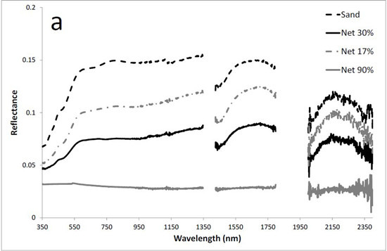
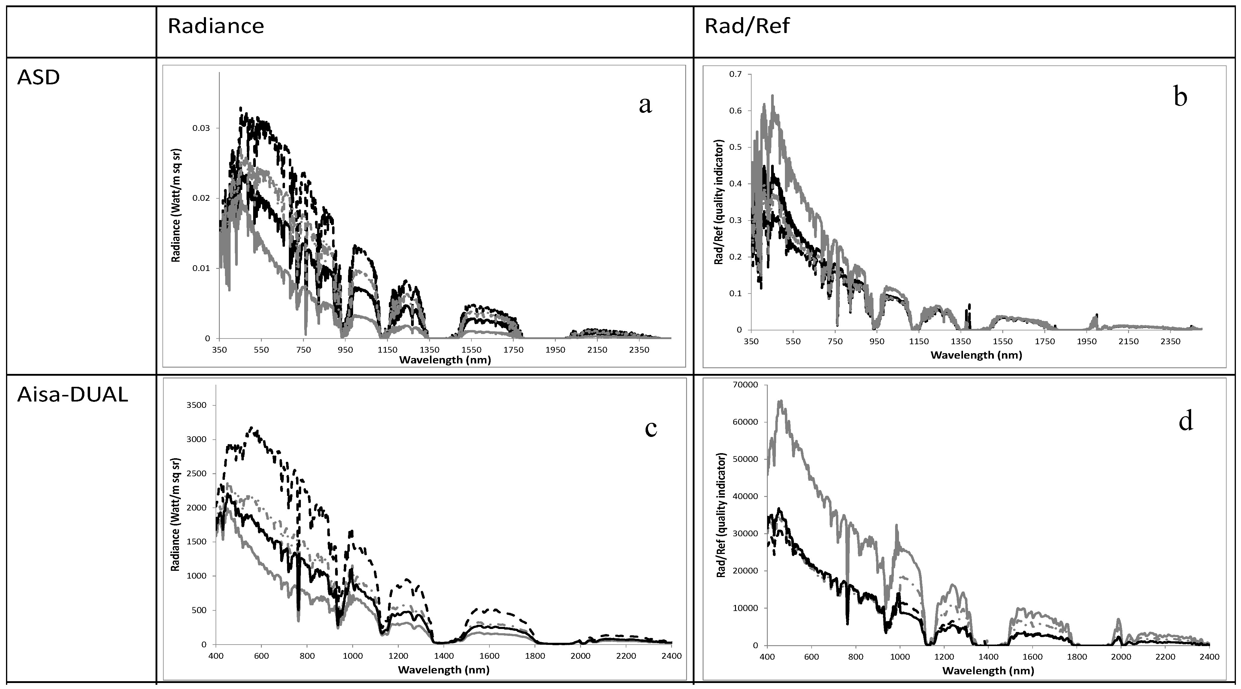
Figure 6.
The radiometric performed for ideal simulated conditions, real at-sensor radiance and Rad/Ref quality indicator calculated by the ground-truth reflectance (ASD SpecPro spectral library) of the SVC net targets. Sand (black dashed line), Net 17% (gray dashed line), Net 30% (black solid line), Net 90% (gray solid line). (a) Simulated (PCMODWIN4.0) full trajectory at-sensor radiance for ASD SpecPro spectral configuration (wavelengths and full-width half-maximum); (b) Calculated Rad/Ref indicator under ideal simulated conditions. (c) At-sensor radiance of the AisaDUAL sensor; (d) Rad/Ref quality indicator calculated by the real radiance and ground-truth reflectance; (e) At-sensor radiance of AHS (VNIR–SWIR) sensor; (f) Rad/Ref quality indicator calculated by the real radiance and ground-truth reflectance; (g) At-sensor radiance of CASI-1500i sensor; (h) Rad/Ref quality indicator calculated by the real radiance and ground-truth reflectance.
In order to provide sufficient input data, ten different sub-regions of interest were selected randomly across each net target and iteratively introduced to the statistical calculation. All examined sensors showed indistinct results which were therefore rejected (
F-test and
t-test significances in
Table 2). Moreover, none presented correlation coefficients meaning that no relationships were found, all of the results were statistically insignificant, and as presented in
Figure 6, the Rad/Ref indicators showed drifted and incorrect sequences in the VNIR region and no overlap in the SWIR region. Therefore, a complete SVC correction process using F1 and F2 (radiometric recalibration stages) was strongly needed.
Table 3 shows the achieved radiometric performance when applying stages F1 and F2.
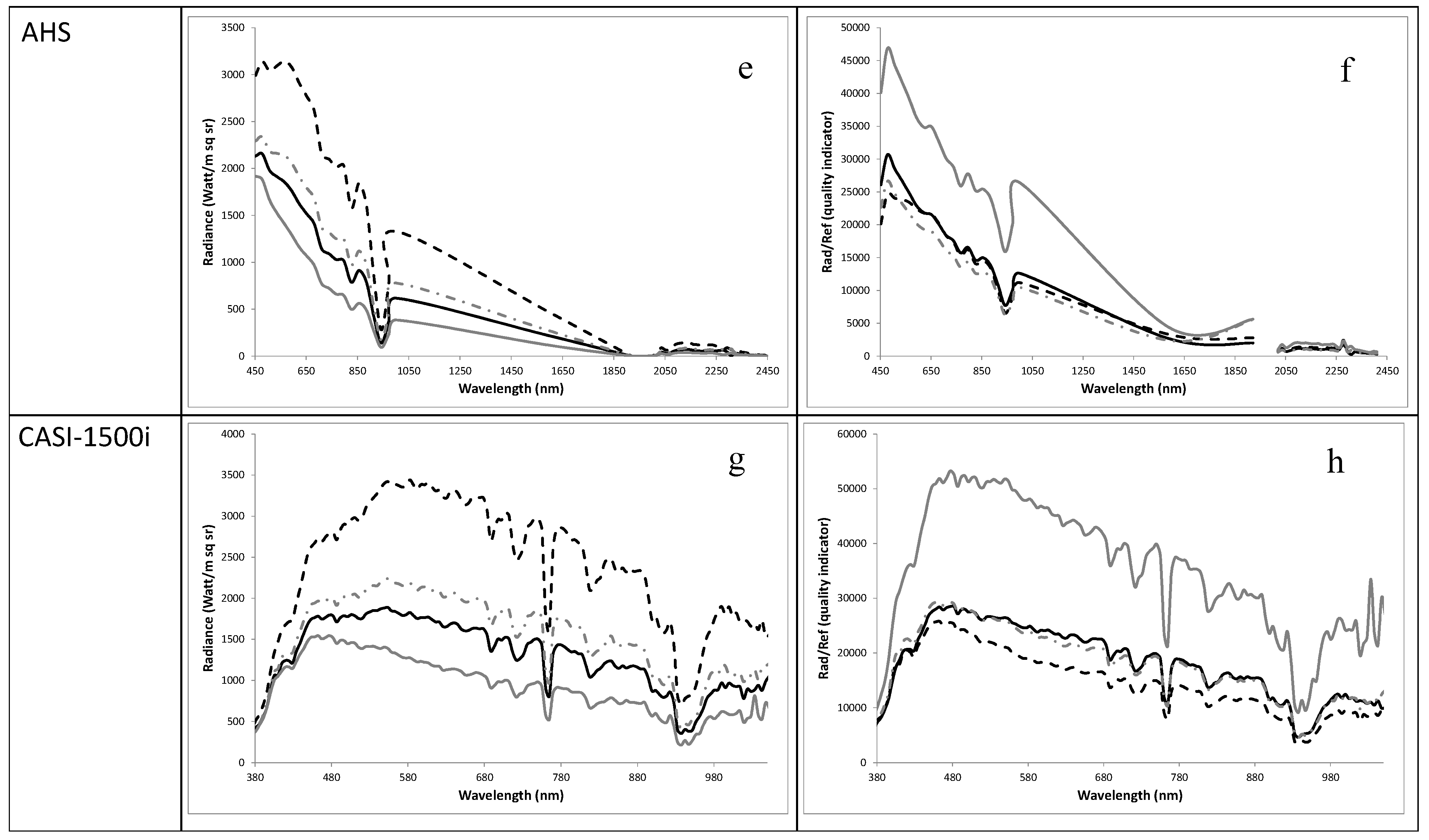
Figure 7 presents the Rad/Ref and RRDF spectra of the corrected at-sensor radiance (stages F1 and F2). As seen, all spectra obey the rules provided in the previous section (
Section 2.3.2) and the corrected radiance can proceed to stages F3 and F4. As both Rad/Ref and RRDF (
Table 3) were statistically significant, the results were accepted and subjected to further processing.
Table 2.
At-sensor radiance quality indicators evaluated according to sc_#1.
Table 2.
At-sensor radiance quality indicators evaluated according to sc_#1.
| Descriptive Statistics | AisaDUAL Radiance | AHS Radiance | CASI-1500i Radiance |
|---|
| Rad/Ref | RRDF | Rad/Ref | RRDF | Rad/Ref | RRDF |
|---|
| VIS | NIR | SWIR | VIS | NIR | SWIR | VIS |
|---|
| N | 4 | 4 | 4 | 3 | 4 | 4 | 4 | 3 | 4 | 3 |
| F test’s Sig. | 0.3 | 0.1 | 0.1 | 0.5 | 0 | 0.1 | 0.08 | 0.5 | 0.5 | 0.3 |
| T test’s Sig. | 0.314 | 0.12 | 0.1 | 0.53 | 0 | 0.2 | 0.1 | 0.5 | 0.3 | 0.1 |
| x mean | 0 | 0 | 0 | NA | 0 | 0 | 0 | NA | 0 | NA |
| y mean | 0.31 | 0.1 | 0 | NA | 1 | 0.1 | 0 | NA | 0.8 | NA |
| Σxy | NA | NA | NA | NA | NA | NA | NA | NA | NA | NA |
| Pearson R | NA | NA | NA | NA | NA | NA | NA | NA | NA | NA |
| Sig. (2-tailed) | NA | NA | NA | NA | NA | NA | NA | NA | NA | NA |
Table 3.
Sensors’ Rad/Ref and RRDF quality indicators, * highlight the accepted significance.
Table 3.
Sensors’ Rad/Ref and RRDF quality indicators, * highlight the accepted significance.
| AisaDUAL | F1 Radiance | F2 Radiance |
| Rad/Ref | RRDF | Rad/Ref | RRDF |
| VIS | NIR | SWIR | VIS | NIR | SWIR |
| N | 4 | 4 | 4 | 3 | 4 | 4 | 4 | 3 |
| F test’s Sig. | 0.03 * | 0.03 * | 0.02 * | 0.04 * | 0.005 * | 0.005 * | 0.005 * | 0.005 * |
| T test’s Sig. | 0.04 * | 0.04 * | 0.04 * | 0.07 | 0.005 * | 0.005 * | 0.005 * | 0.005 * |
| x mean | 0 | 0 | 0 | NA | 0 | 0 | 0 | 0 |
| y mean | 0 | 0 | 0 | NA | 0 | 0 | 0 | 0 |
| Σxy | 46 | 46 | 42 | NA | 68 | 63 | 67 | 49 |
| Pearson R | 0.53 | 0.6 | 0.62 | NA | 0.99 | 0.99 | 0.99 | 0.98 |
| Sig. (2-tailed) | 0.01 * | 0.01 * | 0.01 * | NA | 0.01 * | 0.01 * | 0.01 * | 0.01 * |
| AHS (VNIR-SWIR) | F1 Radiance | F2 Radiance |
| Rad/Ref | RRDF | Rad/Ref | RRDF |
| VIS | NIR | SWIR | VIS | NIR | SWIR |
| N | 4 | 4 | 4 | 3 | 4 | 4 | 4 | 3 |
| F test’s Sig. | 0.04 * | 0.03 * | 0.04 * | 0.04 * | 0.005 * | 0.005 * | 0.005 * | 0.004 * |
| T test’s Sig. | 0.05 * | 0.05 * | 0.05 * | 0.07 | 0.01 * | 0.01 * | 0.01 * | 0.01 * |
| x mean | 0 | 0 | 0 | NA | 0 | 0 | 0 | 0 |
| y mean | 0 | 0 | 0 | NA | 0 | 0 | 0 | 0 |
| Σxy | 47 | 44 | 40 | NA | 64 | 59 | 61 | 49 |
| Pearson R | 0.83 | 0.8 | 0.76 | NA | 0.98 | 0.98 | 0.98 | 0.97 |
| Sig. (2-tailed) | 0.01 * | 0.01 * | 0.01 * | NA | 0.01 * | 0.01 * | 0.01 * | 0.01 * |
| CASI-1500i | F1 Radiance | F2 Radiance |
| Rad/Ref | RRDF | Rad/Ref | RRDF |
| N | 4 | 3 | 4 | 3 |
| F test’s Sig. | 0.04 * | 0.04 * | 0.005 * | 0.004 * |
| T test’s Sig. | 0.05 * | 0.07 | 0.01 * | 0.01 * |
| x mean | 0 | NA | 0 | 0 |
| y mean | 0 | NA | 0 | 0 |
| Σxy | 47 | NA | 64 | 49 |
| Pearson R | 0.83 | NA | 0.98 | 0.97 |
| Sig. (2-tailed) | 0.01 * | NA | 0.01 * | 0.01 * |
Figure 7.
The recalibrated at-sensor radiance and Rad/Ref quality indicator calculated by image reflectance of the SVC net targets: (a) Ground-truth reflectance; (b) Simulated (PCMODWIN4.0) full trajectory at-sensor radiance for ASD SpecPro spectral configuration (wavelengths and full-width half-maximum); (c) Calculated Rad/Ref indicator under ideal simulated conditions. AisaDUAL sensor: (d) Retrieved reflectance; (e) At-sensor radiance. (f) Rad/Ref indicators. AHS (VNIR–SWIR) sensor: (g) Retrieved reflectance; (h) At-sensor radiance. (i) Rad/Ref indicators. CASI-1500i sensor: (j) Retrieved reflectance. (k) At-sensor radiance. (l) Rad/Ref indicators.
Following the SVC processing chain, the next stage was atmospheric correction. The atmospheric correction procedure was examined using the scenarios discussed in
Section 2.3.2. The radiance-corrected image of a selected heading and its extracted L(gain) parameters were applied to different AOI images (
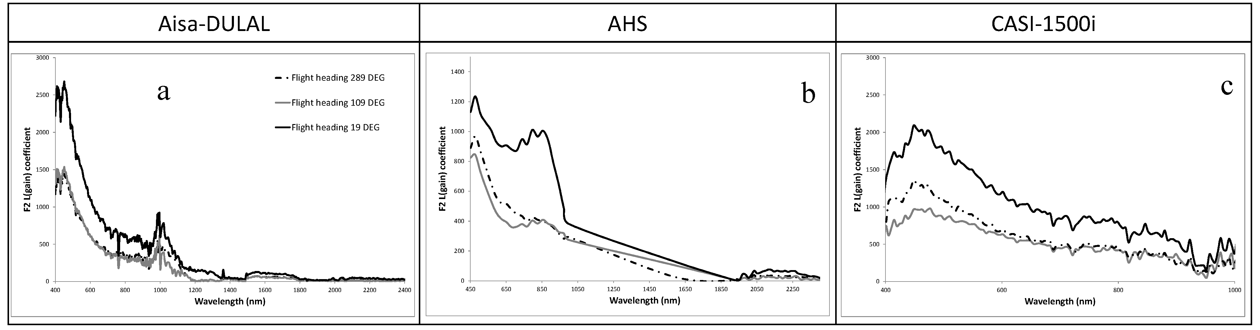
Figure 1). To be discussed in the following sections, the most crucial variance of the extracted L(gain) coefficients were expected in cases of cross-shape heading flights (cs#2 and cs#4), whereas for overlapping heading flights (cs#1 and cs#3) the L(gain) remained stable. This tendency was observed for all of the examined sensors (
Figure 8).
Figure 8.
Extracted F2 L(gain) coefficients for three selected flight headings (289°, 109°, and 19°). Data from (a) AisaDUAL; (b) AHS, and (c) CASI-1500i.
Figure 8.
Extracted F2 L(gain) coefficients for three selected flight headings (289°, 109°, and 19°). Data from (a) AisaDUAL; (b) AHS, and (c) CASI-1500i.
3.1. Radiometric Error
Drawn from the probability distribution function the two methods of evaluation of uncertainty of the data are the Type A error and the Type B error. The type A error method evaluates the uncertainty by the statistical analysis of series of observations, commonly by repeating the measurements and determining the standard deviation of those measurements. Therefore, this method can only be related to uncertainties associated with random effects (e.g., measurement noise). Type B evaluation (of uncertainty) method of uncertainty assessed by means other than the statistical analysis of series of observations and treats both the systematic effects and the random effects, mainly modelled atmospheric variations [
26].
Radiometric error is an uncorrelated and normally distributed random variable which is considered to be the “combined standard uncertainty level” [
27] of a type A error (non-systematic random uncertainties determined by statistical analysis) and type B error (systematic error). Both can be a result of sensor deterioration (of the detector or its surroundings). In the HRS domain, a type A error is linked to sensor noise and a type B error might express radiometric calibration error [
27,
28]. In this study, type B errors were dominant and corrected as the main components of the global uncertainty level and relative radiometric uncertainty level, represented by 95% confidence interval for random error (from normal distribution) or sensitivity coefficient. The sensitivity coefficient was defined as the ratio of the relative standard deviation (calculated for the full spectral region) of an original (input) at-sensor radiance to the ratio of the relative standard deviation of the corrected at-sensor radiance (product of F2 stage).
Moreover, during the data acquisition QI were generated as a standard output, in line with requirements defined within the HYQUAPRO application of uncertainty propagation analysis (UPA). HYQUAPRO developed within the FP7 framework EUFAR (JRA2—HYQUAPRO) to the processing of hyperspectral images (full protocol in DJ2.1.2).
Two cubes of each dataset (each sensor) are provided containing spatial QI and frame related QI information. The spatial QI cube consists of a frequency map of saturated pixels, where a saturated pixel is defined. However, due to an extremely late execution time (12:00 and 16:00 UTC) number of such pixels was very low. The latter criterion also applies to bad pixels, which appear in the saturation layer as stripes, or across the CCD (charge-coupled device) array of the sensor. The frame QI cube, provided by the INTA and NERC (data acquisition teams), holds accumulated saturated pixels per detector pixel, an overall bad pixel map, an interpolated bad pixel map, bad pixels set to NaN, and percent change of the dark current over a given flight line.
During the data processing the relative uncertainty level of the retrieved radiometric coefficient for AisaDUAL, AHS and CASI-1500i according to all examined scenarios (sc_#1,2,3,4) calculated for three selected ground-truth validation targets: tar1—vegetation, tar2—limestone gravel, tar3—concrete and showed in
Table 4.
Table 4.
Relative uncertainty level of the retrieved radiometric coefficient for AisaDUAL, AHS and CASI-1500i according to all examined scenarios (sc_#1,2,3,4) calculated for three selected ground-truth validation targets: tar1—vegetation, tar2—limestone gravel, tar3—concrete.
Table 4.
Relative uncertainty level of the retrieved radiometric coefficient for AisaDUAL, AHS and CASI-1500i according to all examined scenarios (sc_#1,2,3,4) calculated for three selected ground-truth validation targets: tar1—vegetation, tar2—limestone gravel, tar3—concrete.
| Sensor/Correction Scenario Targets | sc_#1 | sc_#2 | sc_#3 | sc_#4 |
|---|
| Tar1 | Tar2 | Tar3 | Tar1 | Tar2 | Tar3 | Tar1 | Tar2 | Tar3 | Tar1 | Tar2 | Tar3 |
|---|
| AisaDUAL | 0.2 | 0.01 | 0.01 | 1.9 | 1.5 | 1.5 | 1.7 | 1.3 | 1.2 | 2.1 | 1.9 | 1.7 |
| Mean Error | 0.073 | 1.633 | 1.400 | 1.900 |
| AHS | 0.4 | 0.1 | 0.01 | 3.5 | 2.1 | 1.8 | 3.1 | 2.5 | 2.1 | 3.9 | 3.6 | 3.5 |
| Mean Error | 0.170 | 2.467 | 2.567 | 3.667 |
| CASI-1500i | 1 | 0.6 | 0.1 | 4.1 | 2.8 | 2.2 | 3.1 | 4.3 | 1.5 | 4.5 | 3.9 | 3.2 |
| Mean Error | 0.567 | 3.033 | 2.967 | 3.867 |
The ideal scenario (sc_#1) presented the best results with the lowest mean error, whereas the non-ideal scenarios (sc_#2,#3,#4) present less accurate results with varying errors relative to the selected sensors. The average uncertainty of the SVC correction for AisaDUAL (1.6%), AHS (3.2%) and CASI-1500i (3.9%) images was ~3%.
Succeeding sc_#1, results derived from the AisaDUAL and the CASI-1500i sensors can be rated by performance in descending order as: (2) sc_#3 in which calibration and validation flight lines keep the same geometry but do not share the coincident acquisitions; (3) sc_#2 in which calibration and validation flight lines do not share the same geometry but preserve the coincident acquisitions and (4) sc_#4 in which calibration and validation flight lines do not share the same geometry and do not share the coincident acquisitions. Results from the AHS sensor can be rated as: (2) sc_#2; (3) sc_#3 and (4) sc_#4.
The scenarios in which calibration and validation flight lines do not share the same geometry but preserve the coincident acquisitions by applying the SVC calibration coefficients (flight line with 289 degree heading) on the cross-shape pattern flight-line coefficients (flight line with 19 degree heading).
Accordingly, in the thematic area sites, an urban region in Salon-de-Provence and a maritime region in the port of Marseille, flight lines with headings of 349 and 226 degrees were used, respectively. The second group illustrated scenarios (sc_#3) in which calibration and validation flight lines keep the same geometry but do not share the coincident acquisitions by applying the SVC coefficients of the flight line with 289 degree heading on the validation flight line with 226 degree heading above the port of Marseille.
The last examination (sc_#4) was performed on the Salon-de-Provence flight line with headings of 349 degrees using the SVC coefficients extracted from the flight line headings of 199 degrees.
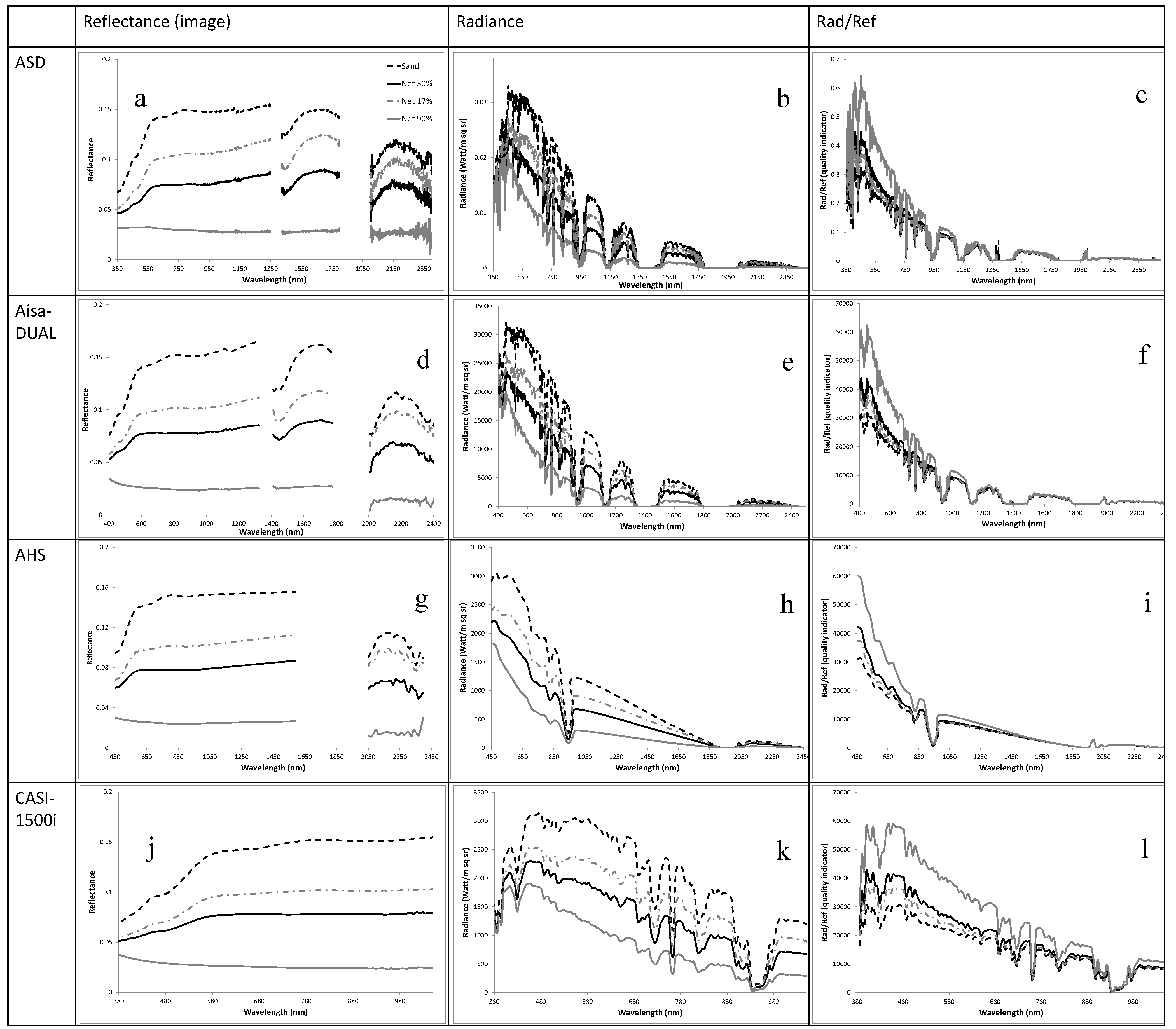
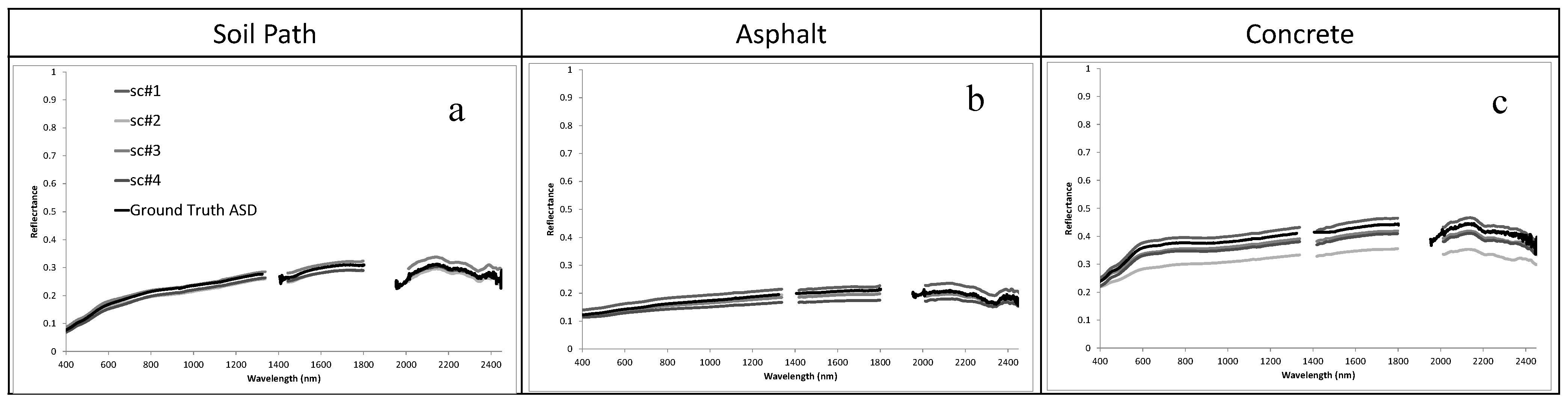
3.2. Accuracy of Reflectance Spectra
The results of the multi-sensor cross-calibration SVC method were examined by comparing the ground-truth spectra of several selected validations. Spectral validation of the reflectance retrieved from the radiance data using the SVC method included selection and examination of three targets at different locations in Salon-de-Provence (urban AOI sites) and near Montpellier (SVC site). In all areas, the following targets were selected: concrete, asphalt, soil path (
Figure 9).
Figure 9.
The ground-truth ASD SpecPro spectra of concrete (a); asphalt (b) and soil path (c) against the reflectance spectra retrieved using the SVC calibration procedure (F1–F4) following scenarios #1, #2, #3, and #4, measured across polygon of 3 × 3 pixels (approximately 15 m2).
Figure 9.
The ground-truth ASD SpecPro spectra of concrete (a); asphalt (b) and soil path (c) against the reflectance spectra retrieved using the SVC calibration procedure (F1–F4) following scenarios #1, #2, #3, and #4, measured across polygon of 3 × 3 pixels (approximately 15 m2).
The quantitative evaluation involved calculating two indicators, the average sum of deviations squared (ASDS; Equations (6), applicable to all HRS sensors) and ASDS spectral variation (ASDS-s; Equation (7), applicable to the AisaDUAL sensor), for all scenarios (
Table 5).
Table 5.
Quantitative evaluation of reflectance information retrieved via ASDS and ASDS-s (in bold) (applicable to AisaDUAL sensor) scores for all investigated scenarios.
Table 5.
Quantitative evaluation of reflectance information retrieved via ASDS and ASDS-s (in bold) (applicable to AisaDUAL sensor) scores for all investigated scenarios.
| Sensor/Correction Scenario Targets | sc_#1 | sc_#2 | sc_#3 | sc_#4 |
|---|
| Tar1 | Tar2 | Tar3 | Tar1 | Tar2 | Tar3 | Tar1 | Tar2 | Tar3 | Tar1 | Tar2 | Tar3 |
|---|
| AisaDUAL | 0.005 | 0.001 | 0.0011 | 0.009 | 0.005 | 0.006 | 0.017 | 0.002 | 0.002 | 0.022 | 0.003 | 0.004 |
| 0.001 | 0.0004 | 0.0001 | 0.005 | 0.001 | 0.001 | 0.006 | 0.001 | 0.001 | 0.007 | 0.001 | 0.002 |
| Mean | 0.0005 | 0.0023 | 0.0027 | 0.0033 |
| AHS | 0.08 | 0.002 | 0.0007 | 0.1 | 0.05 | 0.05 | 0.08 | 0.001 | 0.001 | 0.38 | 0.21 | 0.28 |
| Mean | 0.0275 | 0.0667 | 0.0273 | 0.2900 |
| CASI-1500i | 0.05 | 0.008 | 0.005 | 0.09 | 0.05 | 0.05 | 0.07 | 0.005 | 0.001 | 0.42 | 0.27 | 0.32 |
| Mean | 0.0210 | 0.0633 | 0.0253 | 0.3367 |
The ASDS index examines how one spectrum differs from another, in this case, the SVC-corrected reflectance of each selected target against the ASD of this target as measured in the field. The ASDS was calculated according to [
29] Equations (6.1) and (6.2).
where
is the image reflectance,
is the ASD SpecPro-measured reflectance,
is the number of bands within the spectrum matching the image spectral configuration). The ASDS is composed of both albedo differences (reflectance gain) and spectral noise (spikes or absence of artefacts). When albedo differences are not the decisive parameter of the QA QIs, the spectral noise and artefacts are crucial. [
16] suggested accounting for these spectral variations by subtracting the albedo variation from the total spectral variation (general shape, with noises and artefacts). This was done by estimating ASDS-s by Equation (7).
where
is the offset of ASDS values across the SWIR-1 region (1585–1670 nm) which is a featureless region for most natural (solid) targets and therefore, most probably, represents only the albedo drift.
Figure 9 emphasizes the high accuracy of the retrieved reflectance data by presenting the results of four different scenarios applied to the AisaDUAL imagery data.
The results presented in
Table 4 and
Table 5 show that the SVC approach performed equally well for the selected HRS sensors in both ideal (sc#1 and 3) and non-ideal (sc#2 and 4) scenarios, suggesting that the orientation of the net on the ground is not an important factor. These results are very important for future utilization of the SVC method, where the flight heading and scanning configuration might be detected by the orientation of the SVC ground targets rather than the operator.
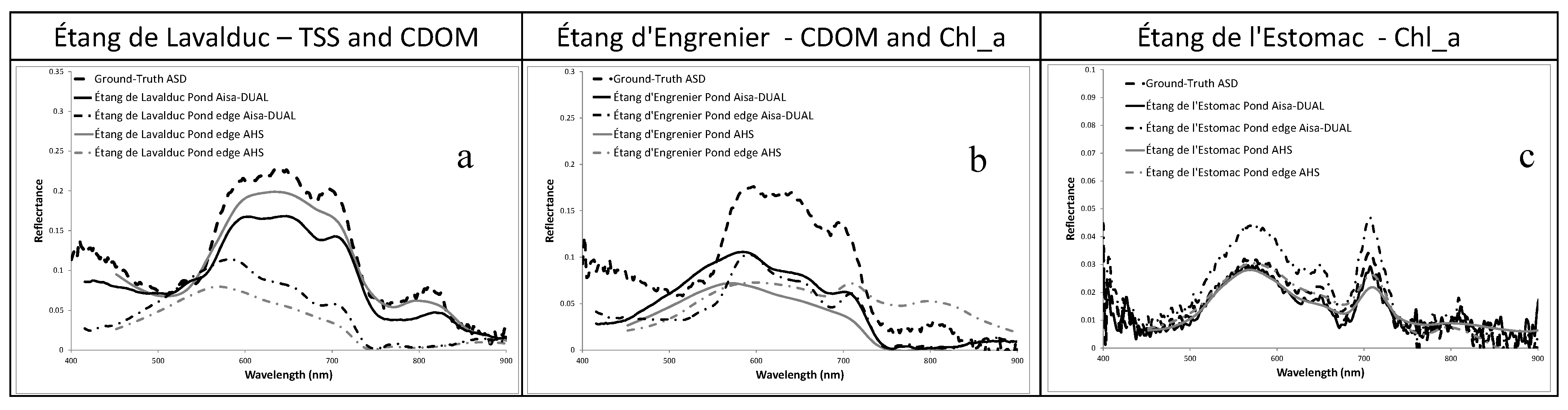
Figure 10 shows the comparison between the ground-truth ASD SpecPro spectra undertaken simultaneously with the data acquisition, and the reflectance retrieved from the selected images. These spectra show good agreement, presenting ASDS values of ~0.005 (
Figure 10).
Figure 10.
The ground-truth ASD SpecPro spectra of water bodies (a) Étang de Lavalduc; (b) Étang d’Engrenier and (c) Étang de l’Estomac versus the reflectance spectra retrieved using the SVC calibration procedure for AisaDUAL and AHS sensors.
Figure 10.
The ground-truth ASD SpecPro spectra of water bodies (a) Étang de Lavalduc; (b) Étang d’Engrenier and (c) Étang de l’Estomac versus the reflectance spectra retrieved using the SVC calibration procedure for AisaDUAL and AHS sensors.
A quantitative comparison between different calibration scenarios (sc_#1,2,3,4) was performed. The suggested quantitative assessment (Equation (12)) was carried out by the structural similarity index (SSIM) to explore a perceptual correspondence between sc_#3 and all other calibration scenarios (sc_#1,2,4). This spatial examination is usually employed on imagery with elusive structural information. The final value of SSIM (1 is total similarity, −1 is total dissimilarity) is the mean value calculated over
local regions (Equation (8)), where m is the mean index value and s denotes the standard deviation [
30].
Two constant values (0.01 and 0.03) were suggested as regulatory factors by [
30]; however; in the present study; the SSIM was unaffected by these factors and insensitive to any possible variations. Therefore; the SSIM algorithm is calculated according to Equation (9); giving a single overall image quality measure.
In practice, a weighted average of the different sub-regions in the SSIM map may segment the image, yet MSSIM is used to evaluate the overall image quality. Estimation of the local statistic is computed by a 3 × 3, 5 × 5 and 7 × 7 pixel-based moving window and then the index values are scaled between 0—complete dissimilarity and 1—complete similarity.
The results (
Table 6) show good agreement (very high MSSIM values) between thematic results of sc_#3 and all other possible calibration scenarios (sc_#1,2,4) regardless of the selected window size (3 × 3, 5 × 5 or 7 × 7). These results confirm the robustness of the proposed multi-source SVC method.
Table 6.
MSSIM overall image quality index computed by a 3 × 3, 5 × 5 and 7 × 7 pixel-based moving-window for AisaDUAL and AHS sensors for all investigated scenarios.
Table 6.
MSSIM overall image quality index computed by a 3 × 3, 5 × 5 and 7 × 7 pixel-based moving-window for AisaDUAL and AHS sensors for all investigated scenarios.
| Scenario | Window-Size | AisaDUAL | AHS |
|---|
| sc_#1 | 3 × 3 | 0.96 | 0.95 |
| 5 × 5 | 0.97 | 0.92 |
| 7 × 7 | 0.96 | 0.94 |
| sc_#2 | 3 × 3 | 0.96 | 0.91 |
| 5 × 5 | 0.94 | 0.93 |
| 7 × 7 | 0.97 | 0.97 |
| sc_#4 | 3 × 3 | 0.97 | 0.96 |
| 5 × 5 | 0.96 | 0.96 |
| 7 × 7 | 0.99 | 0.95 |
3.3. Uncertainty Level
Uncertainty level protocol, such as QA4EO and GUM (Guide to the Expression of Uncertainty in Measurement) provide the HRS data users with simple information to evaluate the fitness-for-purpose for particular application using QI to data and derived products. GUM was developed by the JCGM (Joint Committee for Guides in Metrology), a joint committee of all the relevant standards organizations (e.g., ISO) [
26].
According to the GUM guidelines the calibration processes in the post-launch calibration/validation including uncertainties associated with references, the process of calibration and the “hidden assumptions” in the calibration (e.g., diffuse radiation, radiation geometry, etc.).
The uncertainty level of the solar irradiance model within the diffuser radiance calculation is about 2.5% for all wavelength [
31]. The ground truth averaged reflectance spectra of the validation targets contribute an uncertainty of about 1% [
27].
While the illumination and atmospheric conditions are not stable, all of the measurements described here were made within a few minutes of measurement, ensuring quite constant illumination conditions. The ASD SpecPro is also known to be radiometrically stable over the range of measured ground-truth reflectance values.
The radiative transfer code usually includes many sources of error and uncertainty (e.g., interpolation of LUTs, atmospheric components and parameters, estimation of the atmospheric water vapor content,
etc.). Typically, assessing all significances of the uncertainties (3.5% for all wavelengths) indicated by [
18,
19,
32] and is too complex, and therefore in this study, we used the published relative uncertainties as the upper limit associated with the SVC technique [
16].
The total root mean square (RMS) uncertainty of the SVC correction for AisaDUAL images was 1.5% for the VNIR–SWIR region, for AHS it was 2.5% for the VNIR and 1.7% for the SWIR regions, and for CASI-1500i, it was 1.2% for the VNIR region. The RMS uncertainty of the SVC correction according to GUM for AisaDUAL images was 1.7% for the VNIR–SWIR region, for AHS it was 3.7% for the VNIR–SWIR region, and for CASI-1500i, it was 1.1% for the VNIR region.
4. Discussion
The SVC method demonstrated a proven capability to correct HRS data radiometrically for three different sensors, two platforms and different flight conditions (altitude, heading and time). The multi-HRS sensor multi-platform experience showed that the SVC correction procedure does not rely on these external parameters. Nonetheless, it was found to be sensitive to the flight direction and to the precise protocol used to correct the data and convert them into reflectance units. This is probably related to the fact that flying over the area in question in the same direction as the net setup minimizes the BRDF effects. The SVC method enables a simple QA using two QIs—Rad/Ref, RRDF. These support the HRS data analysis, and provide a realistic and applicable solution to improving the at-sensor data and gaining reliable reflectance information. The fact that none of the sensors met the QA limit values as detected by the Rad/Ref and RRDF indicators demonstrates the importance of the SVC for use as a simple and easy evaluation method. SVC examination performed during the flight mission ensures that uncertainty factors that cannot be modeled in the laboratory calibration will be incorporated into the SVC corrections. Many factors can bias the sensor laboratory calibration during the flight, such as: external conditions belonging to the sensor, the radiation pathway or direction, or the platform used. The assumption that the SVC method is also governed by the flight direction, as part of the anisotropic reflectance characteristics of the sensed area, was also proven in this study. If for some reason the QA is not sufficient, a workflow with concrete stages is proposed to correct the at-sensor data.
Uncertainty values were established in accordance with: HYQUAPRO and GUM. Type A uncertainty was derived using statistical methods, whereas Type B sources have been evaluated by parameters that serve as specifications, comparisons, or calibration data [
33]. The suggested atmospheric correction is performed to correct systematic drift effects (type B error) that occur during data acquisition and, as previously discussed, degrade the radiance accordingly. The SVC, however, cannot deal with the nonsystematic drift (type A error) that may be part of the basic SNR of the sensor (provided by the sensor operators). The opportunity to apply the SVC in a robust way,
i.e., for large net targets, the folding direction and the altitude of the aircraft above the SVC site are less significant; this is a remarkable finding. The study shows that the SVC can be easily applied if a suitable bright area is found and the overpass can be performed in any heading direction dictated by the flight trajectory or the sun’s elevation. Although it is highly recommended that the bright area be featureless, this is not practical. Hence, a bright area with features can also be used as the spectral sequence obtained by the different net densities enables modeling these features out from the calibration. The nets can be easily unfolded in 30 min by two people. The main advantage of the suggested targets is that they are made of the same material with different mixing rates and end up covering the sensor’s entire dynamic range, thus it is important to have more than two SVC nets targets. The two immediate indicators to assess the quality of the data (Rad/Ref and RRDF) based on the reflectance and radiance of the net targets on the ground enable immediate inspection of the data which, if planned ahead, can be done on board the aircraft. In principal, the ground team can measure the reflectance of all nets during the overpass and this information can be transmitted to the airplane. The SVC calibration image can be download from the sensor and processed onboard by applying first radiometric calibration and then the suggested QI parameters (Red/Ref and RRDF). The result can be automatically calculated and provide the operator with the current status of the sensor.
This work adds values to the SVC study conducted by [
16], who first suggested this approach. In addition, it confirms the remarkable results that were obtained through many flight campaigns conducted from 2010 using the SVC approach for the AisaDUAL sensor, which was not subjected to routine laboratory calibration. Those results, based on reflectance information, suggested that the SVC method enables normalization of all sensors producing similar reflectance units that, if needed, can be used across them.


