
Ice Freeze-up and Break-up Detection of Shallow Lakes in Northern Alaska with Spaceborne SAR


Abstract
:
1. Introduction
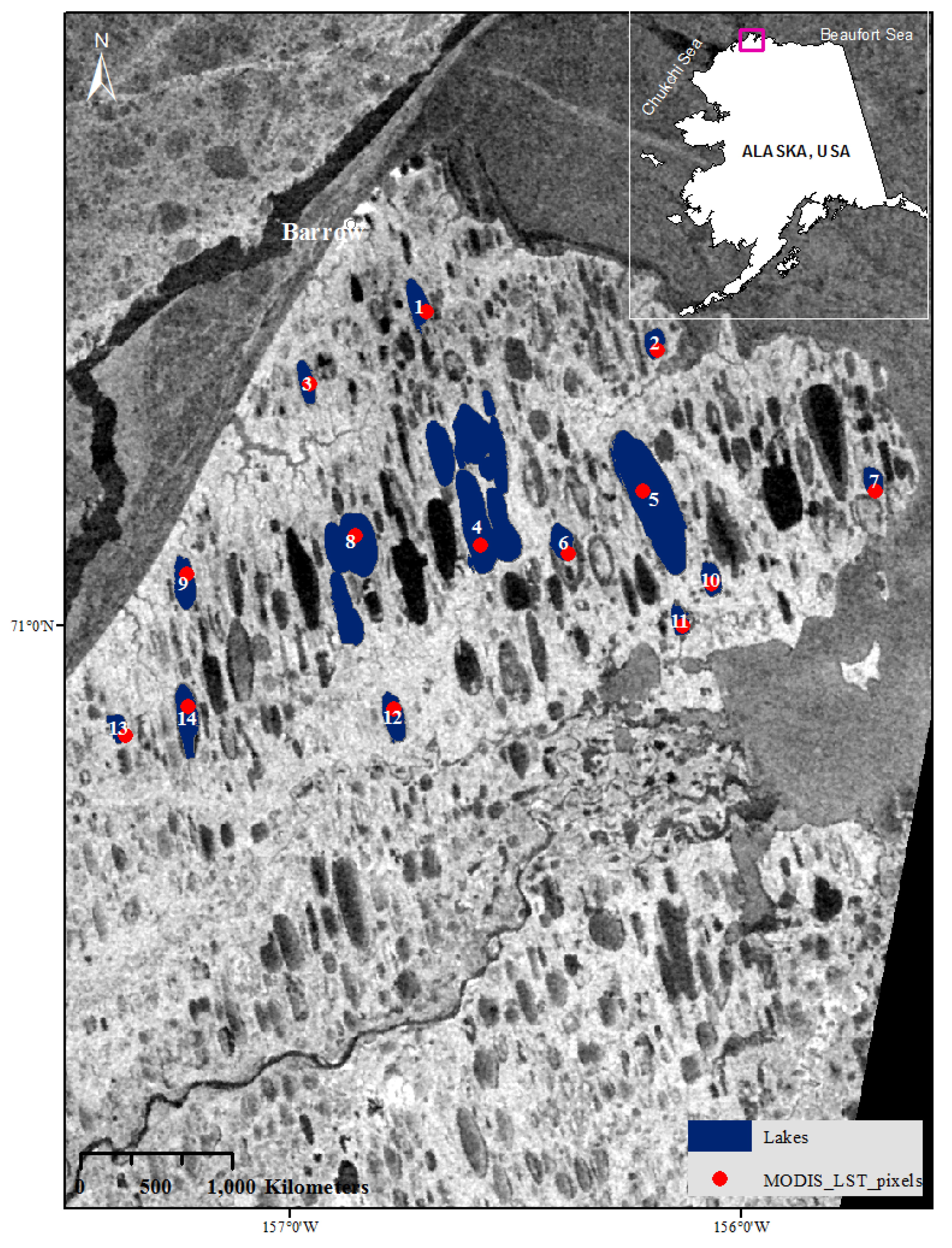
2. Study Area
3. Data and Methods
3.1. Synthetic Aperture Radar (SAR)

| ROI # | Lake Name | Number of ASAR Pixels | Number of RADARSAT-2 Pixels | Lake Type |
|---|---|---|---|---|
| 1 | Ikroavik Lake | 567 | 2098 | coastal/central |
| 2 | Unnamed Lake A | 328 | 1224 | coastal/peripheral |
| 3 | Unnamed Lake B | 390 | 1442 | northern |
| 4 | Lake Sungovoak | 6131 | 23148 | large |
| 5 | Lake Tusikvoak | 3833 | 14416 | deep |
| 6 | Unnamed Lake C | 465 | 1730 | shallow |
| 7 | Unnamed Lake D | 323 | 1234 | western |
| 8 | Sukok Lake | 2913 | 10985 | floating ice cover |
| 9 | Unnamed Lake E | 622 | 2352 | eastern |
| 10 | Unnamed Lake F | 372 | 1410 | inland/peripheral |
| 11 | Unnamed Lake G | 299 | 1103 | inland/central |
| 12 | Unnamed Lake H | 599 | 2232 | southern |
| 13 | Unnamed Lake I | 290 | 1094 | small |
| 14 | Tractor Lake | 813 | 3100 | grounded ice cover |

3.2. Lake-ice Modeling
3.3. Meteorological Data
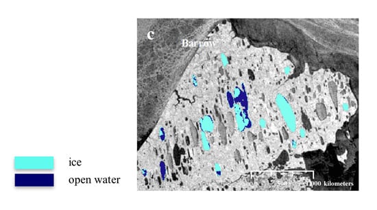
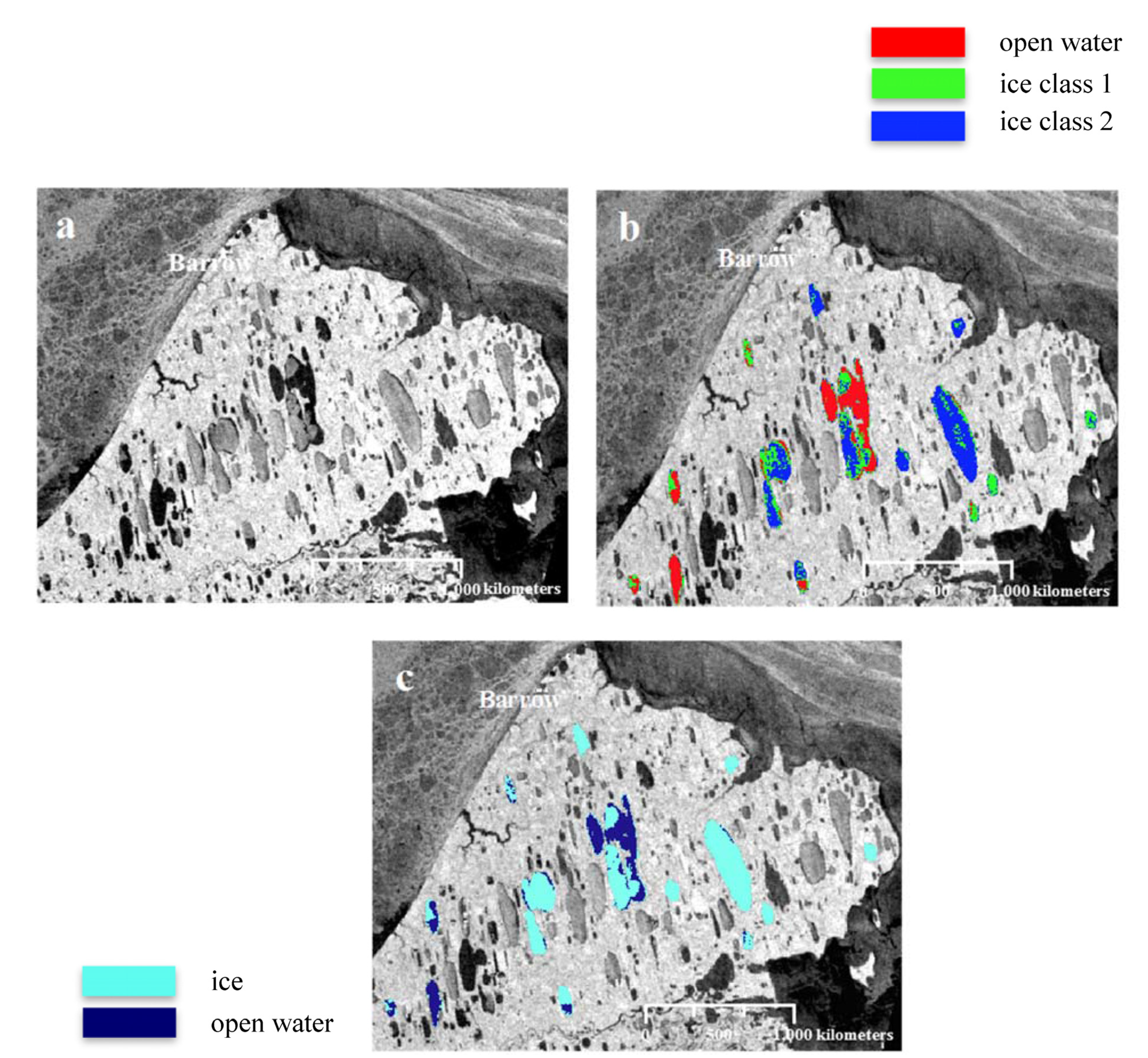
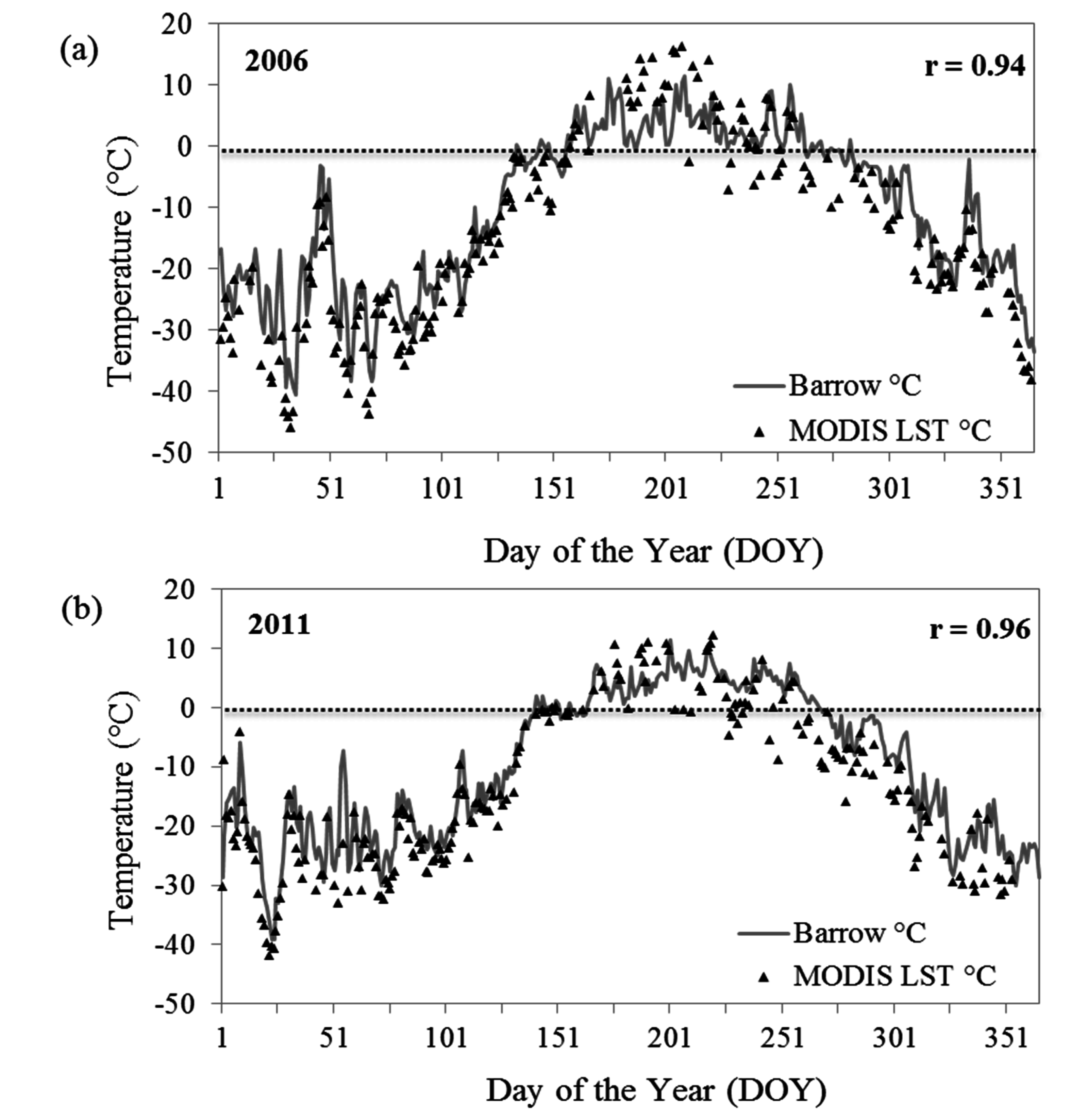
3.4. MODIS Lake/Ice Surface Temperature
4. Results
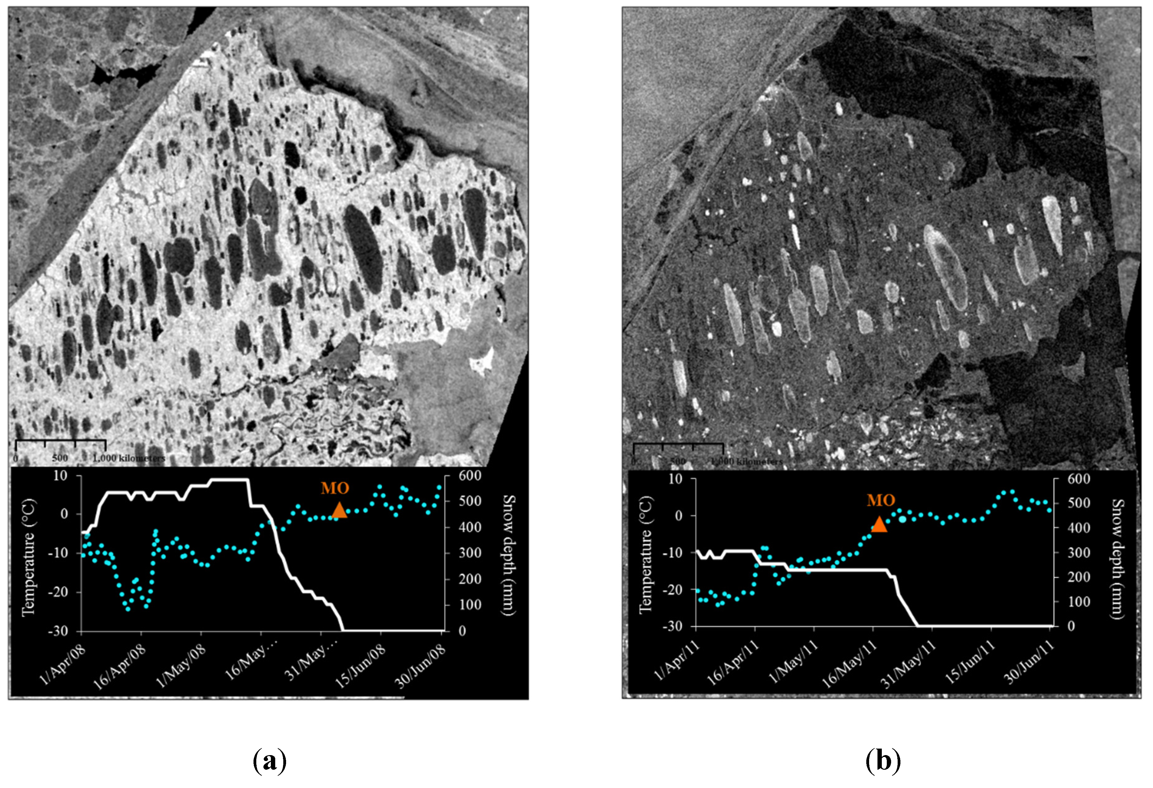
4.1. Freeze-Up
| Year | SAR | CLIMo | Difference Range SAR/CLIMo (# of Days) |
|---|---|---|---|
| 2005 | 258 (255–261) | 270 | 9–15 |
| 2006 | - | 279 | - |
| 2007 | 266 (263–275) | 276 | 1–13 |
| 2008 | 280 (279–283) | 276 | 3–7 |
| 2009 | 276 (271–280) | 273 | 2–7 |
| 2010 | 271 (265–275) | 273 | 2–8 |
| 2011 | 276 (274–280) | 274 | 0–6 |
| Mean FO 2005–2011 | 271 (255–283) | 274 | 0–15 |
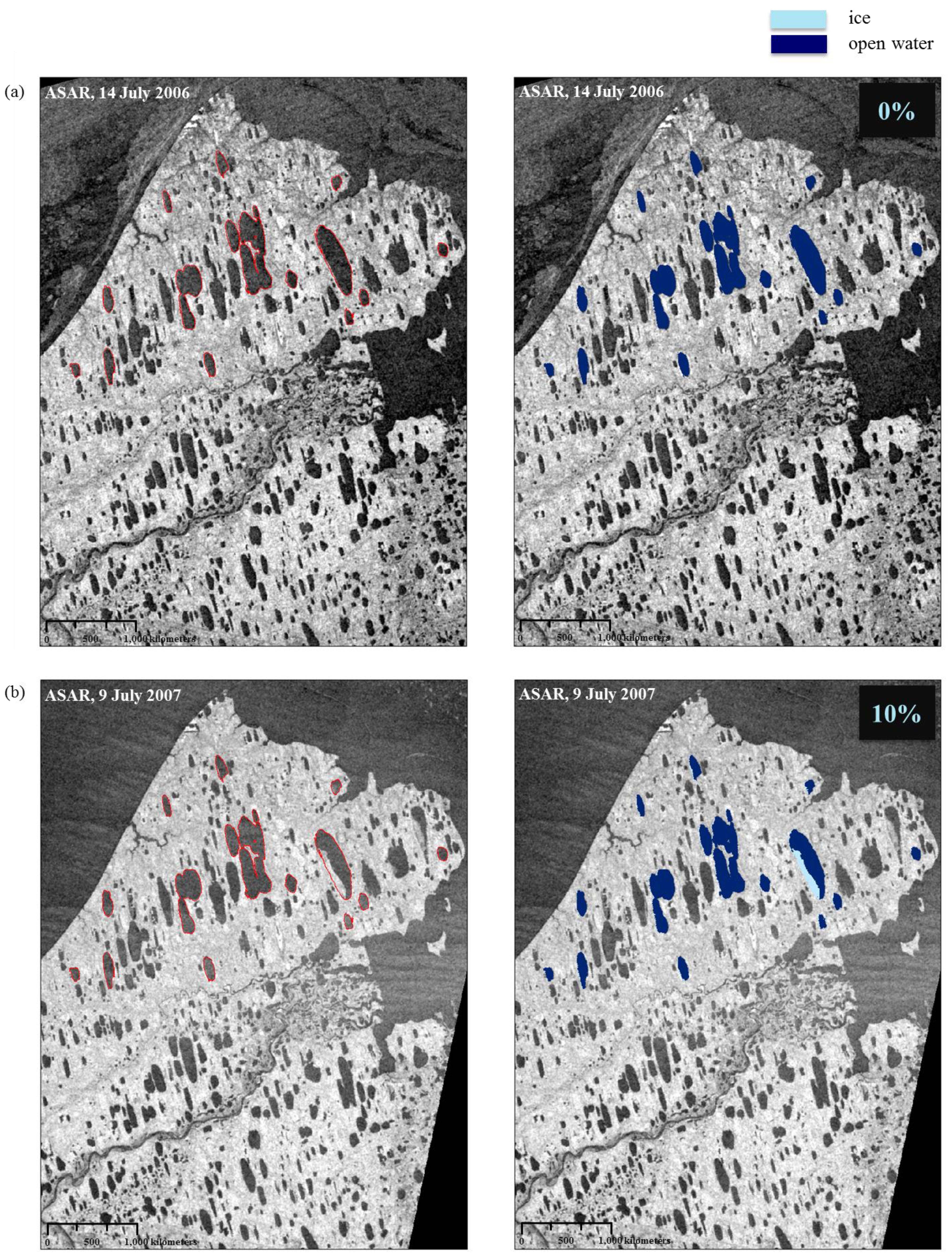
4.2. Break-Up
| Year | SAR | CLIMo | Difference Range SAR/CLIMo (# of Days) |
|---|---|---|---|
| 2006 | 141 (131–151) | 134 | 3–17 |
| 2007 | 141 (136–145) | 144 | 1–8 |
| 2008 | 156 (155–158) | 138 | 17–20 |
| 2009 | 143 (137–149) | 132 | 5–17 |
| 2010 | 147 (144–150) | 145 | 1–5 |
| 2011 | 133 (128–145) | 139 | 6–9 |
| Mean MO 2006–2011 | 143 (128–158) | 136 | 1–20 |
| Year | SAR | CLIMo | Difference Range SAR/CLIMo (# of Days) |
|---|---|---|---|
| 2006 | 194 (189–198) | 193 | 4–5 |
| 2007 | 190 (189–190) | 189 | 0–1 |
| 2008 | - | 186 | - |
| 2009 | 187 (178–190) | 186 | 4–8 |
| 2010 | 195 (192–198) | 194 | 2–4 |
| 2011 | 198 (196–201) | 192 | 4–9 |
| Mean WCI 2006–2011 | 191 (178–201) | 190 | 0–9 |
5. Discussion
5.1. Timing of Key Lake-Ice Events
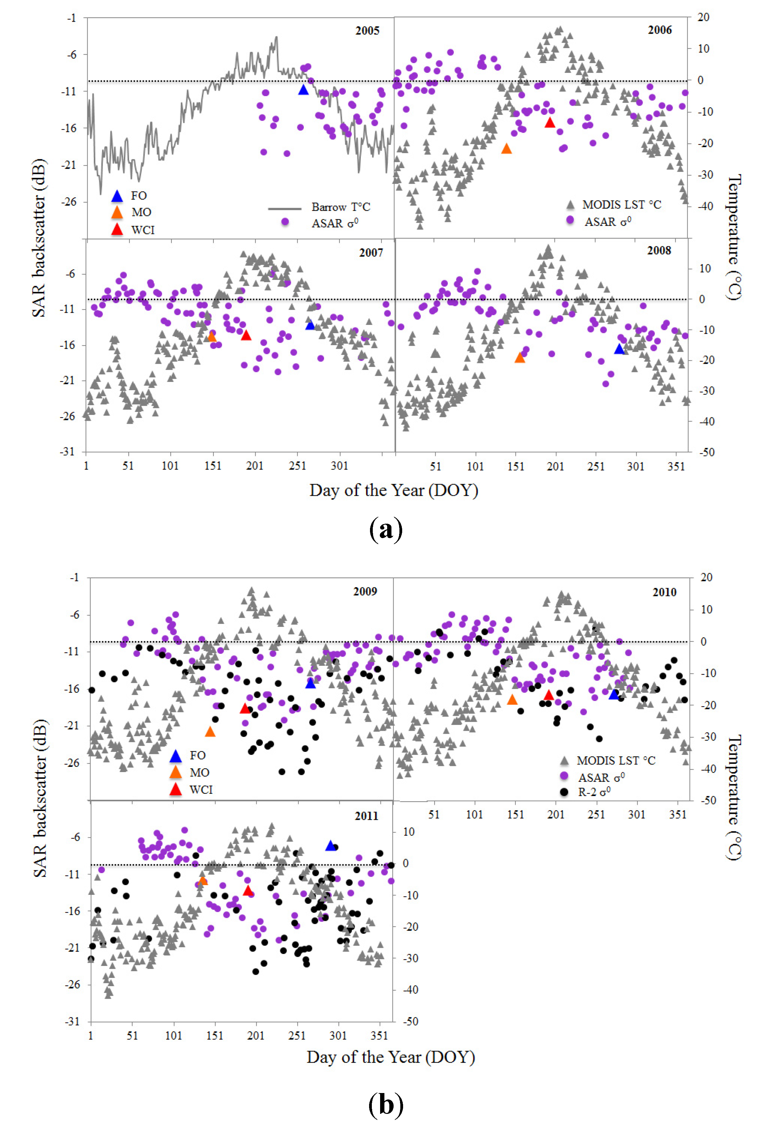
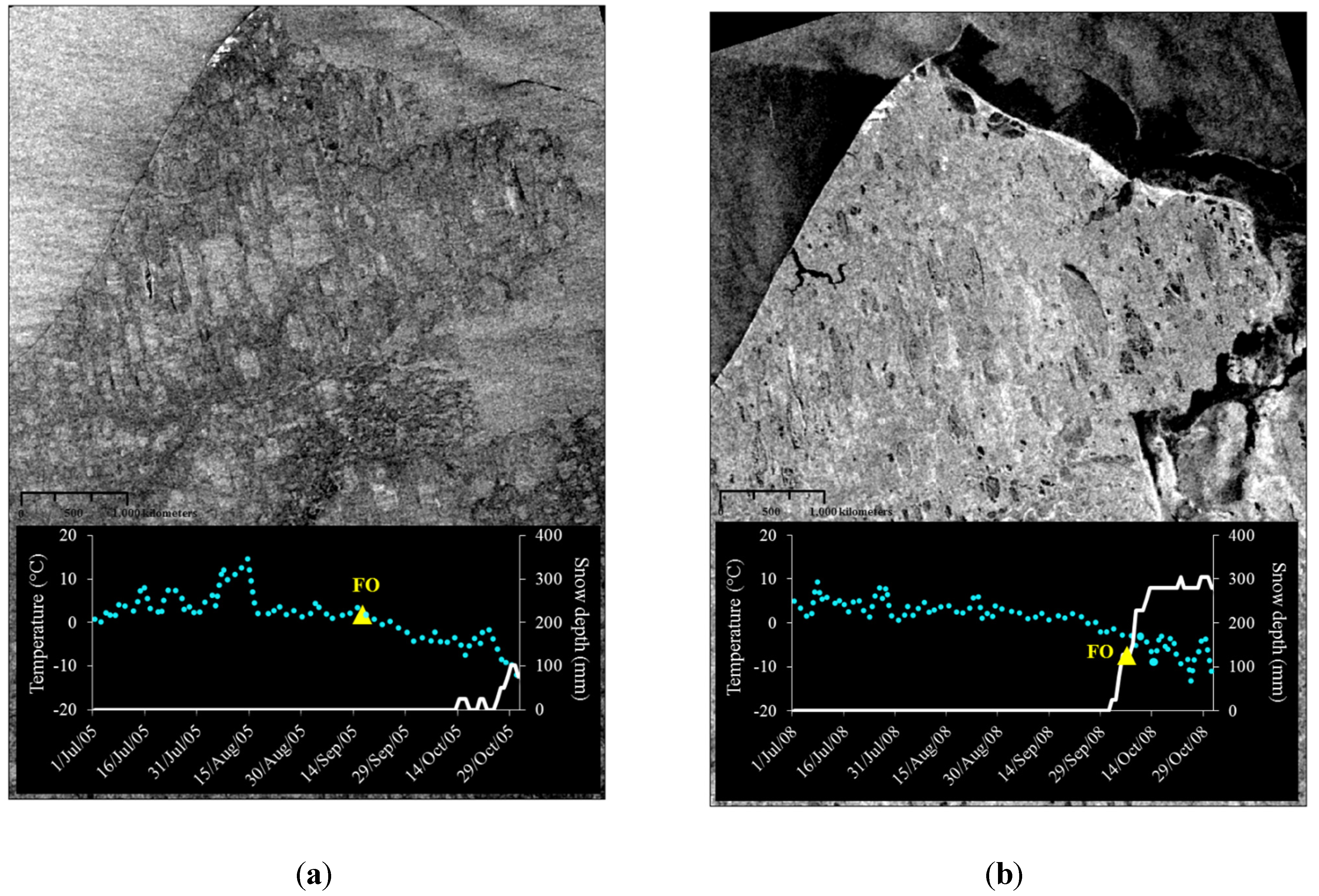
5.1.1. Freeze Onset

5.1.2. Melt Onset
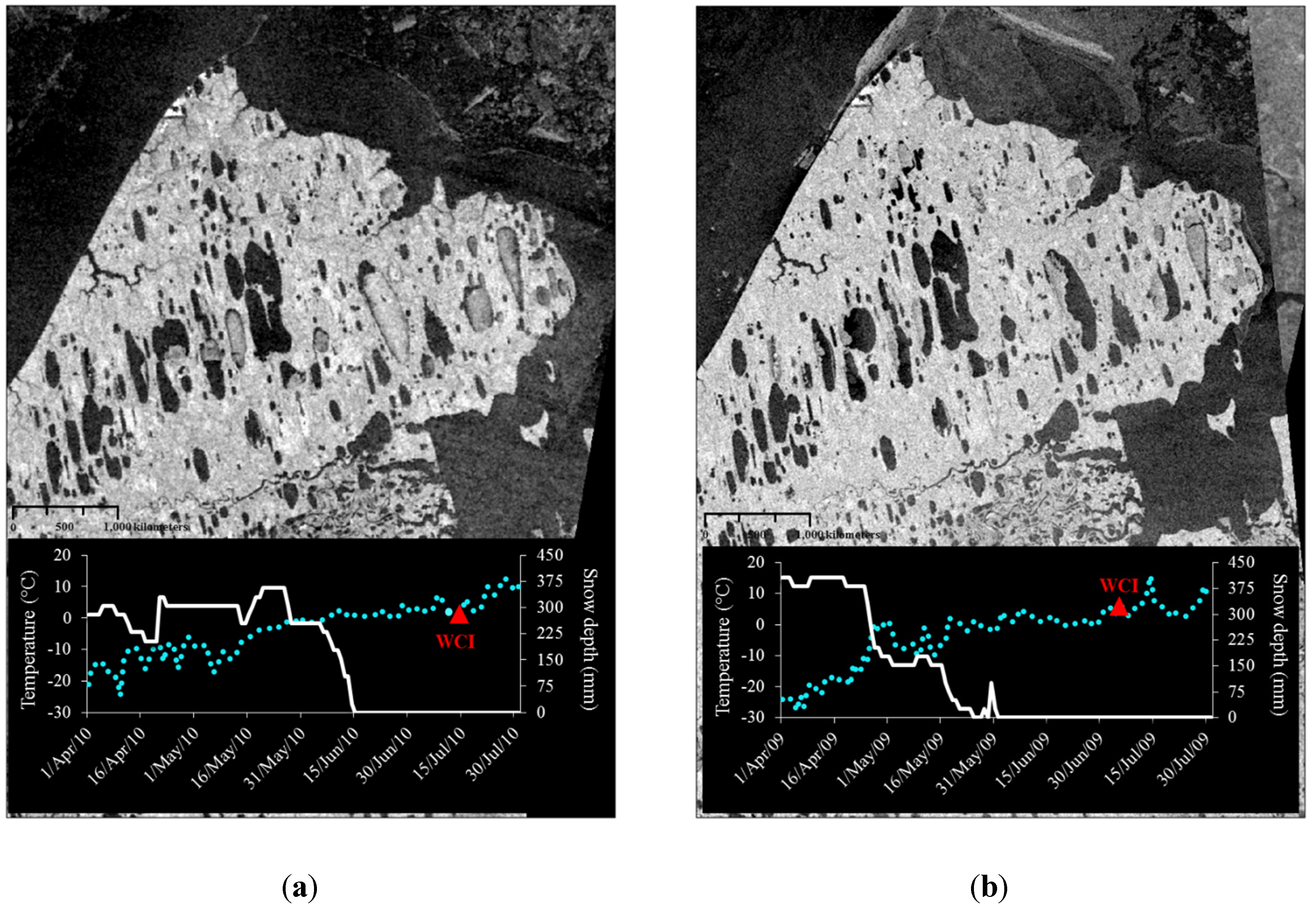
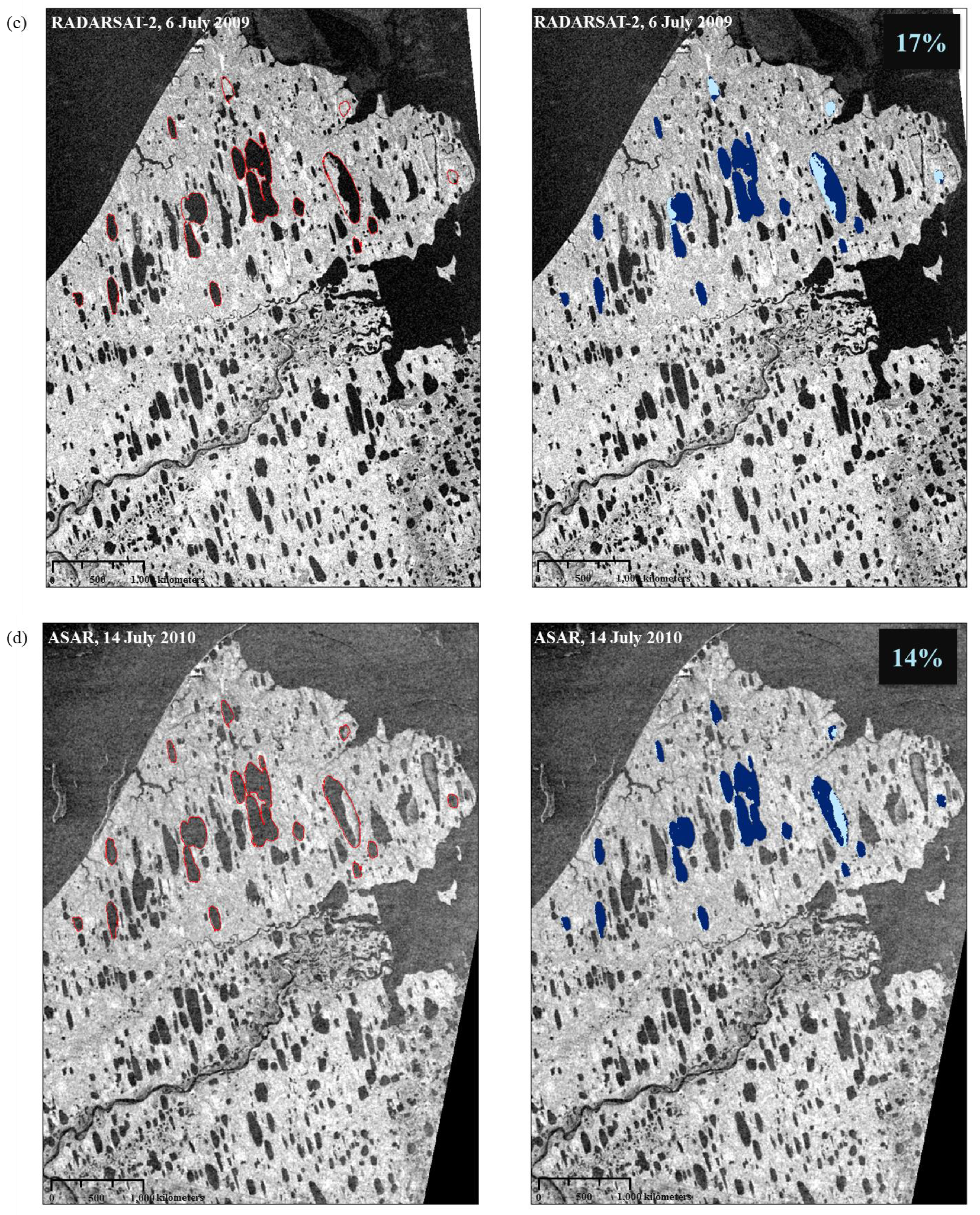
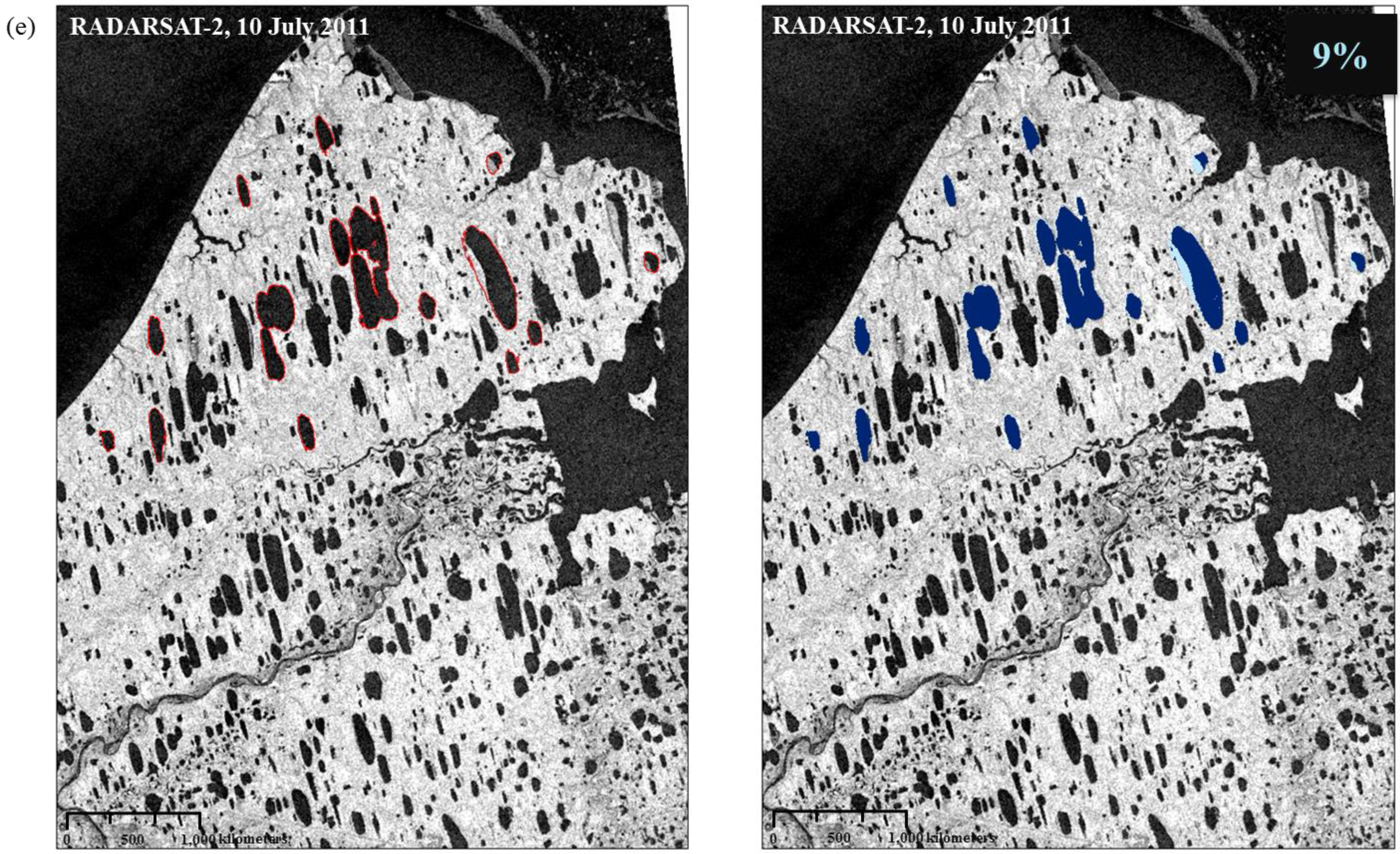
5.1.3. Water-Clear-of-Ice


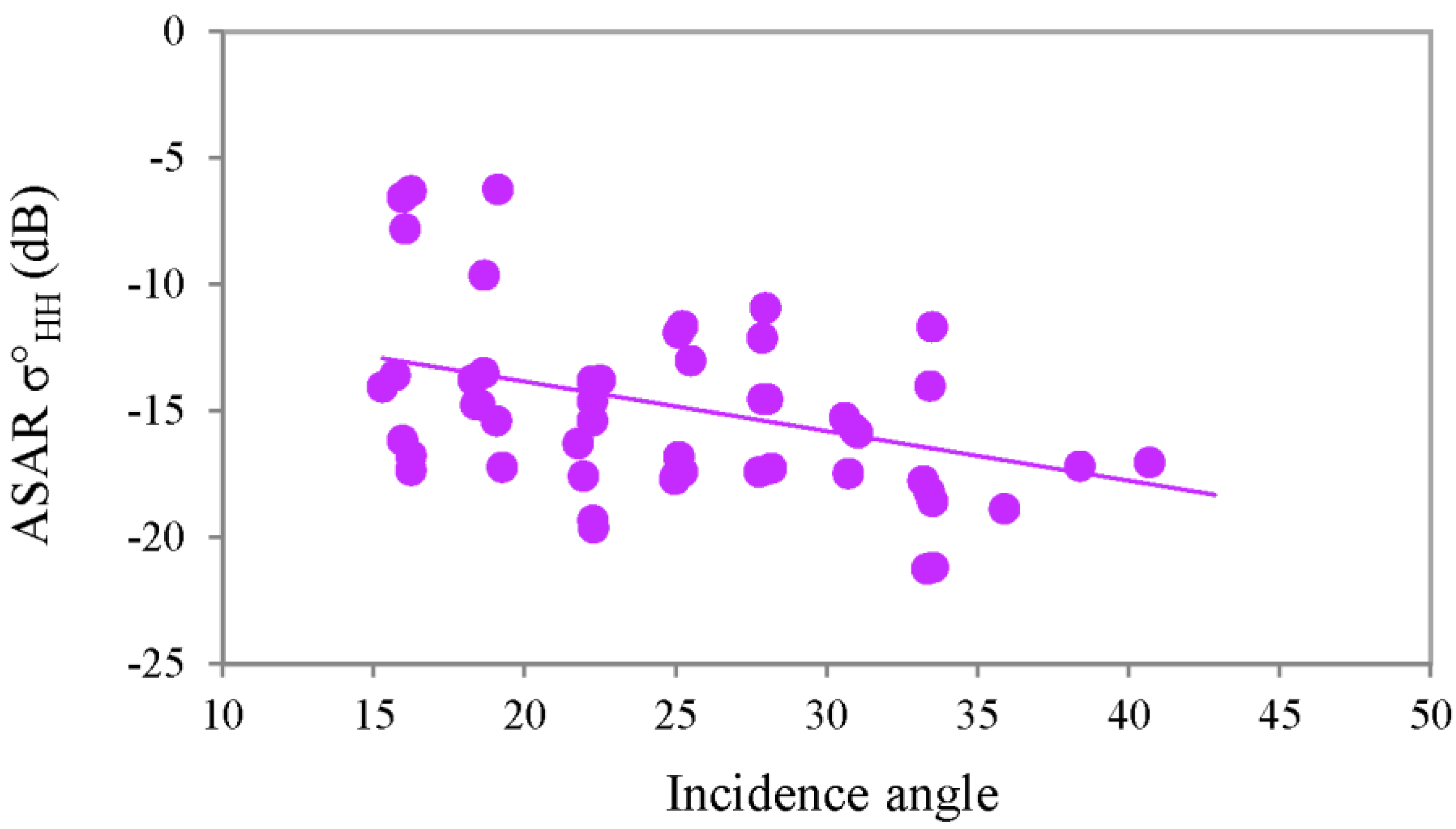
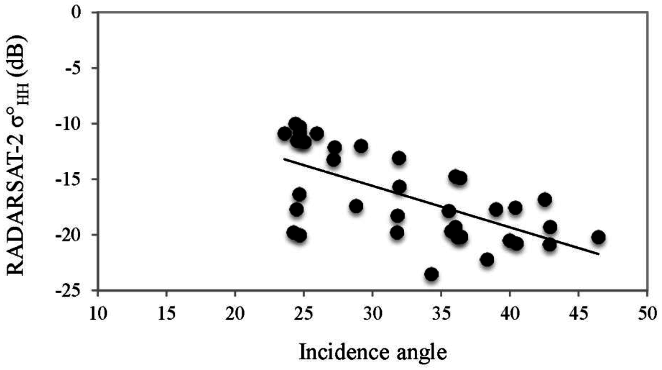
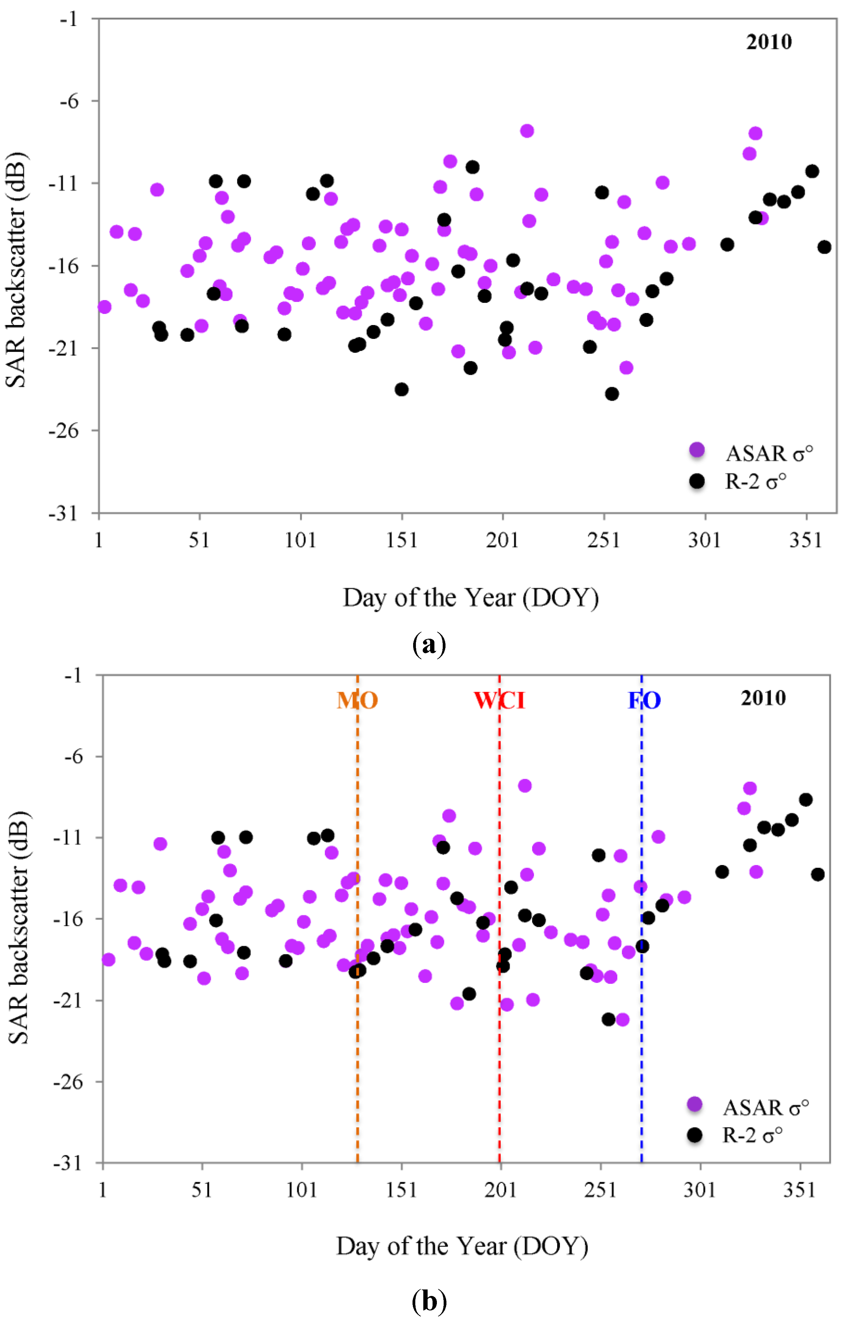
5.2. Backscatter Sensitivity to Incidence Angle and Polarization


| Date of Acquisition | ASAR θ (°) | ASAR σ° (dB) | ASAR Orbit | R-2 θ (°) | R-2 σ° (dB) | R-2 Orbit |
|---|---|---|---|---|---|---|
| 14 February 2010 | 21.78 | −16.31 | DESC | 36.18 | −20.19 | DESC |
| 03 April 2010 | 33.52 | −18.59 | DESC | 36.45 | −20.17 | DESC |
| 08 May 2010 | 35.89 | −18.89 | DESC | 42.88 | −20.85 | DESC |
| 24 May 2010 | 28.32 | −16.82 | ASC | 36.03 | −19.28 | ASC |
| 31 May 2010 | 22.52 | −13.81 | ASC | 34.27 | −23.5 | ASC |
| 21 June 2010 | 28.32 | −16.85 | ASC | 27.15 | −13.22 | ASC |

6. Conclusions
Acknowledgments
Author Contributions
Conflicts of Interest
References
- Sellmann, P.V.; Brown, J.; Lewellen, H.; McKim, H.; Merry, C. The Classification and Geomorphic Implications of Thaw Lakes found in Arctic Alaska; Research Report 344; U.S. Army Cold Regions Research and Engineering Laboratory: Hanover, NH, USA, 1975.
- Li, S.; Jeffries, M.; Morris, K. Mapping the bathymetry of shallow tundra lakes using InSAR techniques. Proc. IGARSS 2000, 5. [Google Scholar] [CrossRef]
- Surdu, C.M.; Duguay, C.R.; Brown, L.C.; Fernández Prieto, D. Response of ice cover on shallow lakes of the North Slope of Alaska to contemporary climate conditions (1950–2011): Radar remote sensing and numerical modeling data analysis. Cryosphere 2014, 8, 167–180. [Google Scholar] [CrossRef]
- Screen, J.A.; Simmonds, I. The central role of diminishing sea ice in recent Arctic temperature amplification. Nature 2010, 464, 1334–1337. [Google Scholar] [CrossRef] [PubMed]
- IPCC. Climate change 2013: The Physical science Basis. Contribution of Working Group I to the Fifth Assessment Report of the Intergovernmental Panel on Climate Change; Stocker, T.F., Qin, D., Plattner, G.-K., Tignor, M., Allen, S.K., Boschung, J., Nauels, A., Xia, Y., Bex, V., Midgley, P.M., Eds.; Cambridge U. Press: New York, NY, USA, 2013; p. 1535. [Google Scholar] [CrossRef]
- AMAP. Snow, Water, Ice and Permafrost in the Arctic (SWIPA) 2011; Arctic Monitoring and Assessment Programme (AMAP): Oslo, Norway, 2011. [Google Scholar]
- Brown, R.; Derksen, C.; Wang, L. A multi-data set analysis of variability and change in Arctic spring snow cover extent, 1967–2008. J. Geophys. Res.: Atmos. 2010, 115. [Google Scholar] [CrossRef]
- Arp, C.D.; Jones, B.M.; Urban, F.E.; Grosse, G. Hydrogeomorphic processes of thermokarst lakes with grounded-ice and floating-ice regimes on the Arctic coastal plain, Alaska. Hydrol. Process. 2011, 25, 2422–2438. [Google Scholar] [CrossRef]
- Ling, F.; Zhang, T. Numerical simulation of permafrost thermal regime and talik development under shallow thaw lakes on the Alaskan Arctic Coastal Plain. J. Geophys. Res. 2003, 108. [Google Scholar] [CrossRef]
- Stephenson, S.R.; Smith, L.C.; Agnew, J.A. Divergent longterm trajectories of human access to the Arctic. Nat. Clim. Chang. 2011, 1, 156–160. [Google Scholar] [CrossRef]
- Hinkel, K.M.; Zheng, L.; Yongwei, S.; Evan, A. Regional lake ice meltout patterns near Barrow, Alaska. Polar Geogr. 2012, 35, 1–18. [Google Scholar] [CrossRef]
- Jeffries, M.O.; Morris, K.; Liston, G.E. A method to determine lake depth and water availability on the north slope of Alaska with spaceborne imaging radar and numerical ice growth modelling. Arctic 1996, 49, 367–374. [Google Scholar] [CrossRef]
- Duguay, C.R.; Prowse, T.D.; Bonsal, B.R.; Brown, R.D.; Lacroix, M.P.; Ménard, P. Recent trends in Canadian lake ice cover. Hydrol. Process. 2006, 20, 781–801. [Google Scholar] [CrossRef]
- Palecki, M.A.; Barry, R.G. Freeze-up and break-up of lakes as an index of temperature changes during the transition seasons: A case study for Finland. J. Clim. Appl. Meteorol. 1996, 25, 893–902. [Google Scholar] [CrossRef]
- Arp, C.D.; Jones, B.M.; Grosse, G. Recent lake ice-out phenology within and among lake districts of Alaska, USA. Limnol. Oceanogr. 2013, 58, 2013–2028. [Google Scholar] [CrossRef]
- Jeffries, M.O.; Morris, K.; Weeks, W.F.; Wakabayashi, H. Structural and stratigraphic features and ERS 1 synthetic aperture radar backscatter characteristics of ice growing on shallow lakes in NW Alaska, winter 1991–1992. J. Geophys. Res. 1994, 99, 22459–22471. [Google Scholar] [CrossRef]
- Duguay, C.R.; Pultz, T.J.; Lafleur, P.M.; Drai, D. RADARSAT backscatter characteristics of ice growing on shallow sub-arctic lakes, Churchill, Manitoba, Canada. Hydrol. Process. 2002, 16, 1631–1644. [Google Scholar] [CrossRef]
- Duguay, C.R.; Lafleur, P.M. Determining depth and ice thickness of shallow subarctic lakes using spaceborne optical and SAR data. Int. J. Remote Sens. 2003, 24, 475–489. [Google Scholar] [CrossRef]
- White, D.M.; Prokein, P.; Chambers, M.K.; Lilly, M.R.; Toniolo, H. Use of synthetic aperture radar for selecting Alaskan lakes for winter water use. J. Am. Water Resour. Assoc. 2008, 44, 276–284. [Google Scholar] [CrossRef]
- Cook, T.L.; Bradley, R.S. An analysis of past and future changes in the ice cover of two high-Arctic lakes based on synthetic aperture radar (SAR) and Landsat imagery. Arct. Antarct. Alp. Res. 2010, 42, 9–18. [Google Scholar] [CrossRef]
- Geldsetzer, T.; Van Der Sanden, J.J. Identification of polarimetric and nonpolarimetric C-band SAR parameters for application in the monitoring of lake ice freeze-up. Can. J. Remote Sens. 2013, 39, 263–275. [Google Scholar] [CrossRef]
- Geldsetzer, T.; Van Der Sanden, J.J.; Brisco, B. Monitoring lake ice during spring melt using RADARSAT-2 SAR. Can. J. Remote Sens. 2010, 36, S391–S400. [Google Scholar] [CrossRef]
- Howell, S.E.L.; Brown, L.C.; Kang, K.-K.; Duguay, C.R. Variability in ice phenology on Great Bear Lake and Great Slave Lake, Northwest Territories, Canada, from SeaWinds/QuikSCAT: 2000–2006. Remote Sens. Environ. 2009, 113, 816–834. [Google Scholar] [CrossRef]
- IGOS. Integrated Global Observing Strategy Cryosphere Theme Report—For the Monitoring of Our Environment from Space and from Earth; World Meteorological Organization: Geneva, Switzerland, 2007; WMO/TD-No. 1405; p. 100. [Google Scholar]
- Mellor, J. Bathymetry of Alaskan Arctic Lakes: A Key to Resource Inventory with Remote Sensing Methods. Ph.D. Thesis, Institute of Marine Science, University of Alaska, Fairbanks, AK, USA, May 1982. [Google Scholar]
- Hall, D.K.; Fagre, D.B.; Klasner, F.; Linebaugh, G.; Liston, G.E. Analysis of ERS 1 synthetic aperture radar data of frozen lakes in northern Montana and implications for climate studies. J. Geophys. Res. 1994, 99, 22473–22482. [Google Scholar] [CrossRef]
- Morris, K.; Jeffries, M.O.; Weeks, W.F. Ice processes and growth history on Arctic and sub-arctic lakes using ERS-1 SAR data. Polar Rec. 1995, 31, 115–128. [Google Scholar] [CrossRef]
- Duguay, C.R.; Pultz, T.J.; Lafleur, P.M.; Drai, D. RADARSAT backscatter characteristics of ice growing on shallow sub-arctic lakes, Churchill, Manitoba, Canada. Hydrol. Process. 2002, 16, 1631–1644. [Google Scholar] [CrossRef]
- Sobiech, J.; Dierking, W. Observing lake- and river-ice decay with SAR: advantages and limitations of the unsupervised k-means classification approach. Ann. Glaciol. 2013, 54. [Google Scholar] [CrossRef]
- Ménard, P.; Duguay, C.R.; Flato, G.M.; Rouse, W.R. Simulation of ice phenology on Great Slave Lake, Northwest Territories, Canada. Hydrol. Process. 2002, 16, 3691–3706. [Google Scholar] [CrossRef]
- Duguay, C.R.; Flato, G.M.; Jeffries, M.O.; Ménard, P.; Morris, K.; Rouse, W.R. Ice-cover variability on shallow lakes at high latitudes: Model simulations and observations. Hydrol. Process. 2003, 17, 3465–3483. [Google Scholar] [CrossRef]
- Jeffries, M.O.; Morris, K.; Kozlenko, N. Ice characteristics and processes, and remote sensing of frozen rivers and lakes. In Remote Sensing in Northern Hydrology: Measuring Environmental Change; Duguay, C.R., Pietroniro, A., Eds.; American Geophysical Union: Washington, DC, USA, 2005; pp. 63–90. [Google Scholar]
- Brown, L.C.; Duguay, C.R. A comparison of simulated and measured lake ice thickness using a shallow water ice profiler. Hydrol. Process. 2011, 25, 2932–2941. [Google Scholar]
- Sturm, M.; Liston, G.E. The snow cover on lakes of the Arctic Coastal Plain of Alaska, USA. J. Glaciol. 2003, 49, 370–380. [Google Scholar] [CrossRef]
- Kheyrollah Pour, H.; Duguay, C.R.; Martynov, A.; Brown, L.C. Simulation of surface temperature and ice cover of large northern lakes with 1-D models: A comparison with MODIS satellite data and in-situ measurements. Tellus A 2012, 64. [Google Scholar] [CrossRef]
- Kheyrollah Pour, H.; Duguay, C.R.; Solberg, R.; Rudjord, Ø. Impact of satellite-based lake surface observations on the initial state of HIRLAM. Part I: Evaluation of remotely-sensed lake surface water temperature observations. Tellus A 2014, 66. [Google Scholar] [CrossRef]
- Duguay, C.R.; Soliman, A.; Hachem, S.; Saunders, W. Circumpolar and Regional Land Surface Temperature (LST) with Links to geotiff Images and netCDF Files (2007–2010); University of Waterloo: Waterloo, ON, Canada, 2012. [Google Scholar] [CrossRef]
- Soliman, A.; Duguay, C.R.; Saunders, W.; Hachem, S. Pan-arctic land surface temperature from MODIS and AATSR: Product development and intercomparison. Remote Sens. 2012, 4, 3833–3856. [Google Scholar] [CrossRef]
- Cheng, B.; Vihma, T.; Rontu, L.; Kontu, A.; Kheyrollah Pour, H.; Duguay, C.R.; Pulliainen, J. Evolution of snow and ice temperature, thickness and energy balance in Lake Orajärvi, northern Finland. Tellus A 2014, 66. [Google Scholar] [CrossRef]
- Brown, L.C.; Duguay, C.R. The response and role of ice cover in lake-climate interactions. Prog. Phys. Geog. 2010, 34, 671–704. [Google Scholar] [CrossRef]
- Jeffries, M.O.; Morris, K. Some aspects of ice phenology on ponds in central Alaska, USA. Ann. Glaciol. 2007, 46, 397–403. [Google Scholar] [CrossRef]
- Ashton, G.D. River and Lake Ice Engineering; Water Resource Publications: Littleton, CO, USA, 1986; p. 485. [Google Scholar]
- Jensen, O.P.; Benson, B.J.; Magnuson, J.J.; Card, V.M.; Futter, M.N.; Soranno, P.A. Spatial analysis of ice phenology trends across the Laurentian Great Lakes region during a recent warming period. Limnol. Oceanogr. 2007, 52, 2013–2026. [Google Scholar] [CrossRef]
- Ulaby, F.T.; Moore, R.K.; Fung, A.K. Microwave Remote Sensing: Active and Passive, Vol. III: From Theory to Applications; Artech House, Inc.: Norwood, MA, USA, 1986; p. 1097. [Google Scholar]
- Nghiem, S.V.; Leshkevich, G.A. Satellite SAR remote sensing of Great Lakes ice cover, Part 1. Ice backscatter signatures at C-band. J. Great Lakes Res. 2007, 33, 722–735. [Google Scholar] [CrossRef]
© 2015 by the authors; licensee MDPI, Basel, Switzerland. This article is an open access article distributed under the terms and conditions of the Creative Commons Attribution license (http://creativecommons.org/licenses/by/4.0/).
Share and Cite
Surdu, C.M.; Duguay, C.R.; Pour, H.K.; Brown, L.C. Ice Freeze-up and Break-up Detection of Shallow Lakes in Northern Alaska with Spaceborne SAR. Remote Sens. 2015, 7, 6133-6159. https://doi.org/10.3390/rs70506133
Surdu CM, Duguay CR, Pour HK, Brown LC. Ice Freeze-up and Break-up Detection of Shallow Lakes in Northern Alaska with Spaceborne SAR. Remote Sensing. 2015; 7(5):6133-6159. https://doi.org/10.3390/rs70506133
Chicago/Turabian StyleSurdu, Cristina M., Claude R. Duguay, Homa Kheyrollah Pour, and Laura C. Brown. 2015. "Ice Freeze-up and Break-up Detection of Shallow Lakes in Northern Alaska with Spaceborne SAR" Remote Sensing 7, no. 5: 6133-6159. https://doi.org/10.3390/rs70506133
APA StyleSurdu, C. M., Duguay, C. R., Pour, H. K., & Brown, L. C. (2015). Ice Freeze-up and Break-up Detection of Shallow Lakes in Northern Alaska with Spaceborne SAR. Remote Sensing, 7(5), 6133-6159. https://doi.org/10.3390/rs70506133