Abstract
Surface models provide key knowledge of the 3-d structure of forests. Aerial stereo imagery acquired during routine mapping campaigns covering the whole of Switzerland (41,285 km2), offers a potential data source to calculate digital surface models (DSMs). We present an automated workflow to generate a nationwide DSM with a resolution of 1 × 1 m based on photogrammetric image matching. A canopy height model (CHM) is derived in combination with an existing digital terrain model (DTM). ADS40/ADS80 summer images from 2007 to 2012 were used for stereo matching, with ground sample distances (GSD) of 0.25 m in lowlands and 0.5 m in high mountain areas. Two different image matching strategies for DSM calculation were applied: one optimized for single features such as trees and for abrupt changes in elevation such as steep rocks, and another optimized for homogeneous areas such as meadows or glaciers. The country was divided into 165,500 blocks, which were matched independently using an automated workflow. The completeness of successfully matched points was high, 97.9%. To test the accuracy of the derived DSM, two reference data sets were used: (1) topographic survey points (n = 198) and (2) stereo measurements (n = 195,784) within the framework of the Swiss National Forest Inventory (NFI), in order to distinguish various land cover types. An overall median accuracy of 0.04 m with a normalized median absolute deviation (NMAD) of 0.32 m was found using the topographic survey points. The agreement between the stereo measurements and the values of the DSM revealed acceptable NMAD values between 1.76 and 3.94 m for forested areas. A good correlation (Pearson’s r = 0.83) was found between terrestrially measured tree height (n = 3109) and the height derived from the CHM. Optimized image matching strategies, an automatic workflow and acceptable computation time mean that the presented approach is suitable for operational usage at the nationwide extent. The CHM will be used to reduce estimation errors of different forest characteristics in the Swiss NFI and has high potential for change detection assessments, since an aerial stereo imagery update is available every six years.
1. Introduction
Knowledge of tree resources and the structure of forests is key for managing various forest functions and services. Information on the third dimension (z component) of 3-d data has become more and more important over the last decade. Forest characteristics are traditionally estimated in forest inventories based on sample plots. The combination of design-based sample inventories and remote sensing data, e.g., satellite data or airborne laser scanning data, reduces estimation errors and makes field-based inventories more efficient [1]. Stereo optical imagery or laser scanning data have tremendous potential for obtaining area-wide three-dimensional data over several thousands of hectares. Their usage in the analysis of forested areas over an entire country opens up new possibilities for biomass estimations [2,3], forest structure analysis [4,5], biodiversity assessment [6,7] and the optimization of forest inventories at a national level [8].
Three-dimensional data can either be acquired with an active laser or radar system, or passively with a camera taking optical images [9]. In forested areas, airborne laser scanning (ALS) is often the method of choice, because ALS can penetrate the forest canopy and is, therefore, the only means of obtaining sub-canopy forest structure and terrain information [10]. ALS data has proven to be the most accurate data for the generation of highly detailed digital elevation models of bare earth, referred to as digital terrain models (DTMs), within forests [11]. Several countries now have or are in the process of acquiring national ALS data to provide this crucial terrain information countrywide (for example Sweden, Netherlands, Denmark, Austria, Switzerland, Slovakia, Czech Republic and Finland). For the generation of digital surface models (DSMs) different input data can be used. For instance, surfaces may be modeled using the first-return of the ALS point cloud or using point clouds coming from stereo aerial or satellite images.
Once a detailed DTM is available, canopy height models (CHMs) can be computed by subtracting bare earth heights from the DSM heights. If the terrain does not change significantly, which is the case in most countries, the same ALS DTM can be used for the generation of CHMs at several time steps. Digital airborne imagery over large areas is typically less expensive to acquire than ALS data [10]. The acquisition of aerial stereo imagery has a long tradition in many countries and such images are used to update topographic maps and for orthophoto production. There are a variety of studies based on digital aerial images for canopy height generation which have been mainly carried out in Canada [12,13], Germany [14,15,16], Sweden [17] and Finland [18,19,20,21].
Since the stereo-images are acquired during regular national campaigns, there is a constant cycle of image acquisition allowing for continued update of CHMs. This updating is very valuable for studies of environmental processes where change detection is of high importance [22]. Since the workflow for the photogrammetric stereo image matching can be highly automated, a constant updating of the CHMs is also feasible. In the case of Switzerland, the national aerial imagery campaign is carried out by the Federal Office of Topography (swisstopo) using Leica ADS 40 and ADS80 sensors. In a cycle of maximum six years, the whole country, with an area of 41,285 km2, is updated with aerial image data during the leaf-on season.
A variety of different algorithms and software packages for high density image matching are available today. The availability of high quality digital image data, efficient image matching algorithms and the ever increasing capabilities of CPUs and GPUs have led to major improvements in the generation of dense point clouds from stereo images. We decided to use the SocetSet “Next-Generation Automatic Terrain Extraction” (NGATE) by BAE systems for this study, because we have a long time experience with this software and a large amount of licenses at our institute. NGATE includes area- and feature-based image correlation at different minification levels, while the feature-based method matches, for example, edge segments and contours, the area-based approach attempts to correlate the grey levels of image patches based on the assumption that they represent some similarity [23]. The two image-matching approaches of NGATE complement each other. Although the matching performance of NGATE would also improve from higher image overlap, it achieves a good compromise between matching quality and calculation time.
To date, most of the studies using image-based point clouds for forest applications have been carried out in small study areas with relatively flat terrain and even-aged forests [10]. In contrast, we present a nationwide assessment over a variety of forests for the first time. Although Switzerland, with an area of 41,285 km2, is a relatively small country, it is dominated by a small-scale mixture of different forest types covering one third of its territory, and is consequently an excellent testing ground for our approach. As vegetation height is the most important proxy for a wide range of forestry variables, we focus in our analysis on the accuracy and agreement of modeled tree and canopy heights. The main objectives of the present study are: (1) to demonstrate the highly automated workflow to calculate a nationwide surface model out of regular national aerial images; (2) to evaluate the accuracy and completeness of this digital surface model, which is a prerequisite for its subsequent usage; and (3) to present the potential of this data for National Forest Inventories.
2. Material and Methods
2.1. Study Area
Switzerland is a mountainous country of 41,285 km2 area with a diverse topography covering an altitudinal range between 200 and 4500 m a.s.l. [24]. The highest elevations can be found in the Alps in the south and southeastern part of Switzerland. Running from west to east, on the northern side of the Alps, is the Swiss Plateau, where most of the settlement and urban areas are located. The Jura Mountains, which are generally lower than the Alps, are located on the northwestern border of Switzerland and are more rural in character.
Switzerland is characterized by a mixture of different land uses, which are described in the federal land use statistics [25]. Four broad designations are distinguished: settlement and urban areas (8% of the surface area), agricultural areas (36%), wooded areas (forest and woods, 31%) and unproductive areas (lakes and rivers, unproductive vegetation, rocks and screes, glaciers and perpetual snow, 25%) [25]. Forested areas consist of 43% pure coniferous, 18% mixed coniferous, 12% mixed deciduous, 24% pure deciduous and 3% other forests according to the third NFI, covering the period of 2004–2006 [26].
2.2. Image Data
To obtain nationwide coverage, stereo aerial images from regular flight campaigns of the Federal Office of Topography (swisstopo) were used. Swisstopo has two flight programs, one for updating of the topographic landscape model (TLM) [27], usually acquiring images in the leaf-off season in order to also map infrastructure in forests, and one for orthophoto production [28], usually in the leaf-on season (May–September). The strategy is to cover 1/6 of Switzerland for each program annually. This implies that for a complete leaf-on image coverage of the country a maximum six year period has to be considered. Consequently, for the purpose of the present study, image data from 2007 to 2012 were used (Figure 1).
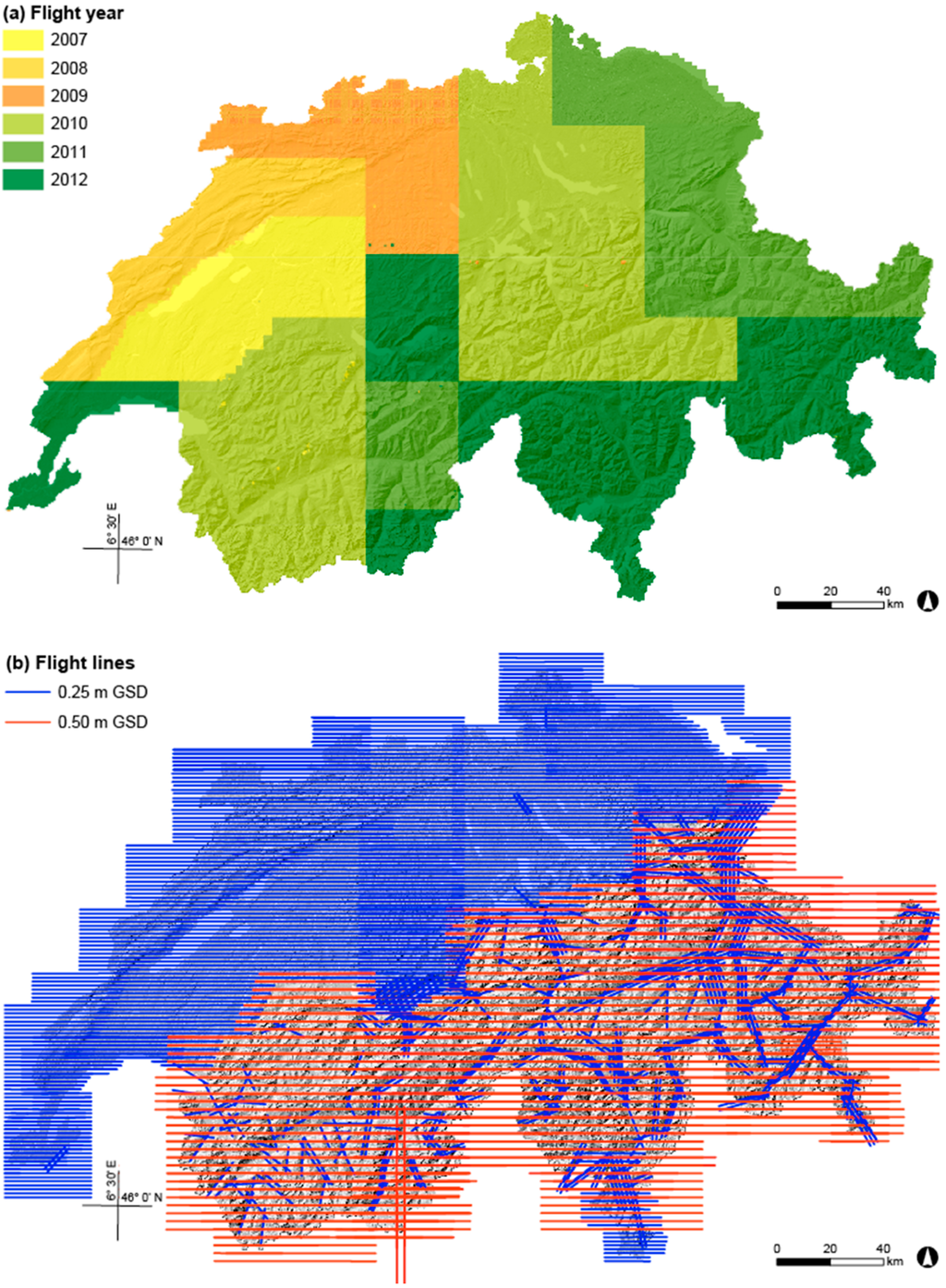
Figure 1.
Image data used: (a) Coverage of ADS40/ADS80 images acquired in 2007–2012, (b) flight lines for the image acquisition for the entire of Switzerland. The imagery was acquired with a GSD of 0.25 m at lower altitudes (denser flight lines) and a GSD of 0.50 m at higher altitudes in the mountainous regions (less dense flight lines).
Over this time frame, three different sensors were in operation. 2007 was the last year swisstopo used the ADS40-SH40 sensor. This sensor collects, at nadir (0°), three spectral bands (blue, green and red), and forward-looking red, green and near infrared (14°, 16° and 18°). Two Pan bands are collected by looking −14° backwards and 28° forwards. The ADS40-SH52 sensor has been used since 2008, with an additional ADS80-SH82 sensor since 2009. These sensors collect four spectral bands (blue, green, red and near infrared) at nadir (0°) and four spectral bands (blue, green, red and near infrared) by looking backward (−16°). Technical details for the different sensor configurations can be found in Appendix A, Table A1.
Swisstopo makes use of two different ground sample distances (GSDs) (Figure 1). In the Jura Mountains, the Swiss Plateau, the pre-alps and along mountain valleys, images have a GSD of ~25 cm. In the Alps, the GSD is ~50 cm. The photogrammetric pre-processing (level 1 generation of raw image data, aerial triangulation (AT) and calculation of RGB and CIR band combinations) is done by swisstopo with the Leica GPro 4.2 software package and image data is provided including camera calibration and orientation data. The orientation accuracy (x, y, z) is reported to be ±1 pixel GSD.
2.3. Generation of the Digital Surface Model (DSM)
The entire workflow for the generation of surface models is highly automated (Figure 2). To distribute calculations over a range of different processing machines, the country was divided into 165,500 blocks of 0.5 × 0.5 km. To avoid edge effects, a buffer of 100 m was added to all sides of the blocks, resulting in an area of 0.7 × 0.7 km for the actual image matching. The blocks were intersected with the stereo footprints of the ADS image stripes, and the distances from the center of each block to the flight lines of the ADS image stripes were calculated. Since the stripes overlap by 50%, in the best case, two stripes for one block are available: one stripe with a shorter distance from the center of the block to the nadir line of the stripe (hereafter 1st most nadir stripe) and a possible second stripe, with a larger distance to the nadir line of the stripe (hereafter as 2nd most nadir stripe). The 1st most nadir stereo image stripes had the highest priority for the matching process for each block since obliqueness effects due to the central perspective of the images are reduced. The 2nd most nadir stereo image stripes were used in cases where image matching on the 1st most nadir stereo image stripes was not successful. The list of all image blocks was managed in a central database to maintain an overview of the ongoing image matching processes. When matching started for a particular block, it stopped being available for other processing machines. After the matching procedure was completed, the block was labeled as finished. Sixteen processes (using 16 virtual Windows7 64bit PCs with 2 cores, 2GB RAM and 2.67 GHz on a Citrix Xen environment) were running parallel on two HP Pro Workstations. The image data was available through a 1 Gb intranet from a central image server.
Image matching was performed using SocetSet 5.6 digital mapping software. The combination of the SocetSet “Next-Generation Automatic Terrain Extraction” (NGATE) by BAE Systems and the stereo line scanning data from the ADS sensors gave the best performance with respect to quality and completeness of image matching and correlation speed. As part of the NGATE, matching is performed for every pixel using area-matching and edge-matching algorithms [29,30]. Although NGATE computes an elevation for every pixel, a fixed spacing must be defined to resample the internal irregular NGATE point cloud to the desired density. No information is available on the interpolation algorithm. Spacing was set to 1 m for the images with 0.25 m and 0.5 m GSD. Only matched raster points were exported from SocetSet as ASCII and then converted to LAS format.
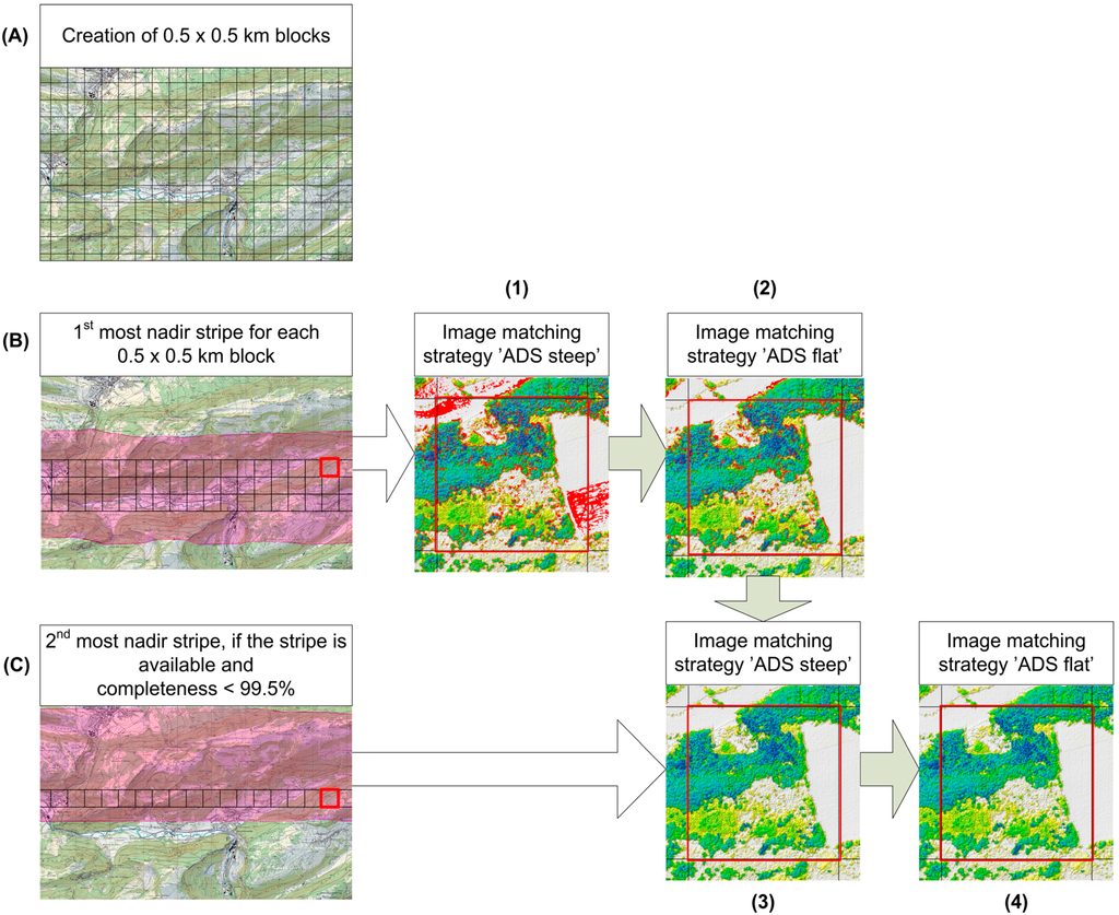
Figure 2.
Image matching workflow. (A) Rasterizing into 0.5 × 0.5 km blocks; (B) selecting the stripe with the smallest distance from nadir to the centre of the block; and (C) selecting the stripe with the second smallest distance from nadir to the center of the block (1) The result after the matching process for the block using the 1st most nadir stereo stripe and the “ADS steep” image matching strategy. Red areas in the image could not be matched. The completeness for this block is 84%. (2) The result after applying the “ADS flat” matching strategy. At 91%, the completeness threshold is still not fulfilled. (3) The result after matching using the 2nd most nadir stripe and the “ADS steep” strategy (completeness 96%) and (4) the final DSM after “ADS flat” strategy with a matching completeness of 96%.
Within SocetSet several correlation strategies for different image contents (e.g., urban, flat homogeneous, hilly and steep areas) are provided. To reach a high level of completeness of the matched points, some of these matching strategies were adapted. We used two different matching strategies (Table 1): “ADS steep”, which is optimized for steep areas and very heterogeneous surfaces with a broad range of different slopes (Figure 3a,b), and “ADS flat”, which is optimized for homogenous areas with little contrast (Figure 3c,d). When matching with the 1st most nadir stereo image stripes using the “ADS steep” strategy was finished, the proportion of successfully matched points was calculated. In one block of 500 × 500 m the maximum of matched points at a grid spacing of 1 m is 250,000. We defined the level of completeness to be reached by 99.5%. If this completeness value was not reached, the “ADS flat” strategy was applied. All additionally matched points with this strategy were then added to the point cloud resulting from the initial “ADS steep” strategy. If the proportion of successfully matched points was still below the threshold of 99.5%, the same procedure was followed using the 2nd most nadir stereo image stripe. Information regarding the stereo image stripe and the strategy used for its calculation was then assigned to each point of the point cloud.

Table 1.
Parameter sets of the two image matching strategies used in the image correlation workflow. The algorithm iterates seven times using the pyramid levels of the images. The seven values listed in the table correspond to the number of iterations.
| Parameter | Strategy 1 “ADS Steep” | Strategy 2 “ADS Flat” |
|---|---|---|
| (1) Number of iterations | 7 | 7 |
| (2) Minification level used | 64-32-16-8-4-2-1 | 64-32-16-8-4-2-1 |
| (3) Image correlation window size [pixel] | 15-15-15-15-11-11-11-11 | 13-13-13-13-13-13-13 |
| (4) Edge matching window [pixel] | 9 × 7-9 × 7-9 × 7-9 × 7-9 × 7-9 × 7-9 × 7 | 9 × 7-9 × 7-9 × 7-9 × 7-9 × 7-9 × 7-9 × 7 |
| (5) Image correlation search distance [pixel] | 21-19-19-19-19-21-21 | 21-15-15-15-15-15-15 |
| (6) Edge matching search distance [pixel] | 13-13-13-15-15-21-21 | 13-13-13-15-15-15-15 |
| (7) Positive spike slope limit [°] | 60-60-40-40-60-60-85 | 20-20-20-20-20-20-20 |
| (8) Negative spike slope limit [°] | 60-60-40-40-40-40-30 | 10-10-10-10-10-10-10 |
| (9) Slope limit [°] | 60-60-60-60-60-85-85 | 60-60-60-60-60-60-60 |
| (10) Smaller window size reduction [pixel] (1) | 0-0-2-2-4-4-4 | 0-0-0-0-0-0-0 |
| (11) Image buffer size [pixel] | 128-128-128-128-128-192-256 | 224-224-224-224-224-288-352 |
| (12) X parallax difference cut-off value [pixel] | 1-1-1-5-10-20-30 | 1-1-1-1-1-1-1 |
| (13) Minimum correlation coefficient difference | 0.180-0.180-0.175-0.170- 0.165-0.160-0.155 | 0.130-0.130-0.125-0.120-0.115-0.110-0.105 |
(1) The actual window correlation size corresponds to the difference of parameter (3) and parameter (10). A smaller window is used in areas with many elevation discontinuities.
Image-matching was done using only one image pair at a given time, which allowed for better control over the amount of matched pixels. Since the green-red-near infrared (CIR) band combination produced the least number of errors, especially in forested regions and in high alpine glacier regions, the two CIR stereo images (backward 16° and nadir 0°) were used for image matching for all of Switzerland. With the exception of the case of the ADS40-SH40 image data from 2007 where the combination of PAN (backward 14°) and RGB (nadir 0°) was used for the matching, because CIR band combination was not possible with this focal plate configuration.
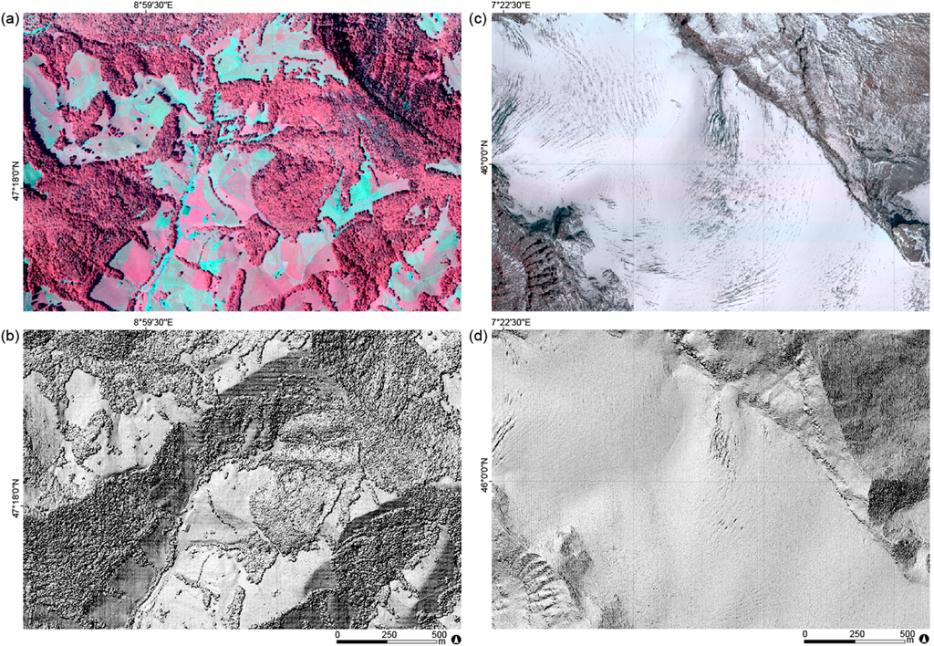
Figure 3.
Examples of the performance of the two different correlation strategies: “ADS steep”, optimized for steep areas and very heterogeneous surfaces such as forest canopies (a) input CIR image and (b) shaded relief of the resulting DSM and “ADS flat”, optimized for homogeneous areas with little contrast such as glaciers (c) input CIR image and (d) shaded relief of the resulting DSM.
2.4. Reference Data for Accuracy Assessment of the Digital Surface Model (DSM)
2.4.1. Topographic Survey Points
A total of 198 topographic survey points, planimetic fixpoints of the new Swiss national topographic survey LV95 [31], were used to assess the absolute accuracy of the digital surface model (Figure 4). They cover the whole country on a more or less regular grid, and are reported to have an absolute accuracy of 3 to 5 cm.
2.4.2. Stereo Measurements of the National Forest Inventory
In the framework of the Swiss NFI, continuous landscape variables are interpreted on the same ADS40/ADS80 stereo imagery, which was used for the digital surface modeling. These stereo measurements are carried out on a rectangular sampling grid of 1.4 km × 1.4 km, using interpretation clusters of 50 m × 50 m, for details see [32,33]. Each interpretation cluster consists of 25 equally spaced lattice points (see Appendix F). A photo interpreter measures the elevation of each lattice point hitting the surface using a 3D softcopy station and assigns a land cover class to each point [34]. For this study, 195,784 measured lattice points, covering 11 land cover types, were used to assess the agreement of the digital surface model. Image matching of water surfaces was not possible since spectral signatures of neighboring pixels were very similar or waves on the water surface led to different reflectance within an image pair; as such this land cover type was excluded from further analyses (Table 3). The values of the four pixels surrounding the lattice points of the stereo measurements were extracted from the digital surface model for comparison with the stereo measurements. For objects with a low object height (herb and grass, rock, sand, stones and visible earth, sealed surfaces, glaciers, firn and snow), the values of the stereo measurements were compared with the minimum value of these four pixels, and for objects with a high object height (trees, shrubs and buildings), the maximum value was used. Only values where the same ADS40/ADS80 image stripe was used for the stereo measurements and the generation of the digital surface model were used in the agreement analysis.
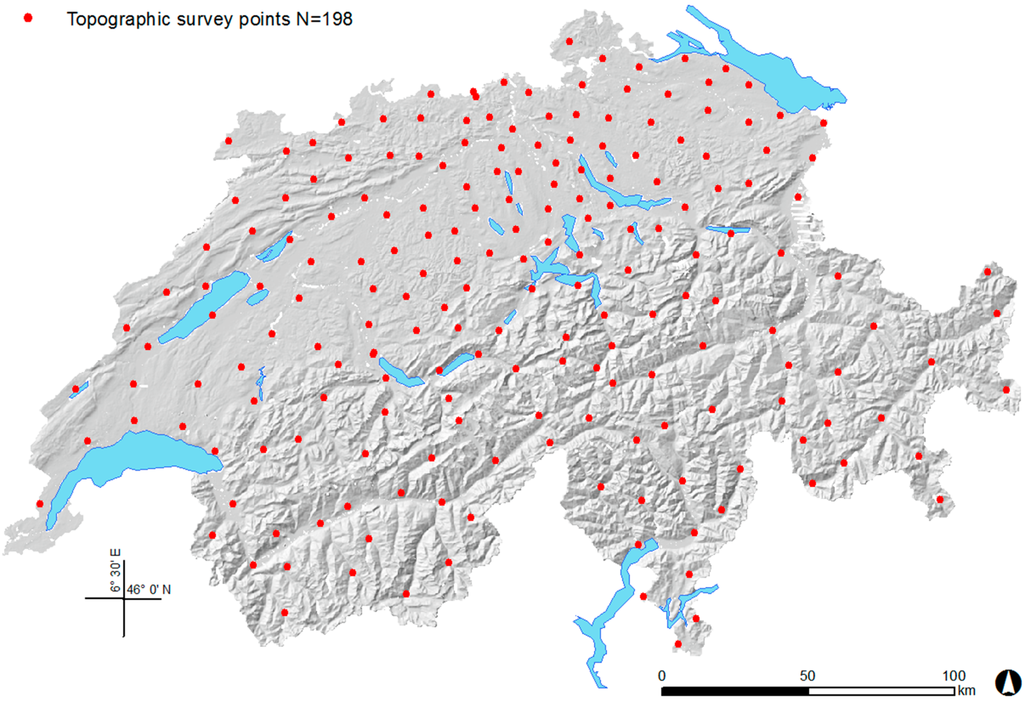
Figure 4.
Reference data for accuracy assessment. The 198 topographic survey points of the national triangulation network were used for an independent error analysis.
2.5. Accuracy Assessment of the Digital Surface Model (DSM)
Knowledge of the accuracy and completeness of the nationwide DSM over different land cover types is crucial for its subsequent usage. Therefore, vertical accuracy assessments were carried out using two reference data sets (topographic survey points and stereo measurements). First, the difference in elevation between the digital surface model and the reference data set was calculated. Because the DSM deviations were not normally distributed, e.g., [35,36] robust accuracy measures described by Höhle and Höhle [37] were used. These included the median, the normalized median absolute deviation (NMAD) and the 68.3% and 95% sample quantiles. For better comparison with other data sets two root mean square errors (RMSE) were calculated, one for the whole sample size and one with outlier correction, where a threshold value of ±3 × RMSE was applied for outlier exclusion. All calculations were done with the open source statistical software R [38]. Analyses were conducted only for the sample of successfully matched image points.
2.6. Generation of the Canopy Height Model (CHM)
By subtracting the digital terrain model swissALTI3D provided by swisstopo from the calculated digital surface model, a normalized digital surface model (nDSM) was generated. The swissALTI3D of swisstopo is based on ALS data with an overall point density of 0.5 points per m2 [39], has a resolution of 2 m which was resampled to 1 m. To obtain the canopy height model, the topographic landscape model TLM provided by swisstopo was used to mask out houses, settlement areas and water bodies.
2.7. Comparison with Terrestrial Measurements of Tree and Canopy Height
2.7.1. Tree Height of Single Trees
Within the ongoing 4th inventory of the Swiss NFI, the heights of a total of 3109 trees belonging to the upper canopy layer were measured using a Vertex ultrasonic hypsometer. Field measurements were conducted between 2009 and 2013, and are spread over the whole country. The coordinates of the tree stem location at breast height were acquired with a Trimble GeoXH (with an average accuracy after post-processing of ±1 m), enabling a comparison with the values of the CHM. Within a 2.5 m radius buffer around each stem, the maximum height values of the CHM were extracted and compared to the tree height of the corresponding measured trees. Only those trees with at least 15 pixels that could be matched within the 2.5 m buffer (93% of all measured trees) were used for the analysis. In addition, only measurements where the tree height was measured later than the date of the image acquisition were included in the analysis. To know how precisely the trees were measured in the field, double measurements within the NFI of 117 deciduous and 324 coniferous trees were compared.
2.7.2. Canopy Height at Plot Level
Individual tree heights measured in the 4th NFI were used to estimate the maximum canopy height at the circular NFI plot level of an area of 500 m2. The maximum values of these terrestrial measurements (only a sub-sample of the trees on the plot is measured—one to three upper layer trees per plot) were then compared to the maximum values of the CHM within the sample plot area. We analyzed the data for different development stages, species mixtures and stand structures.
3. Results
3.1. Generation of Digital Surface Model (DSM)
The nationwide DSM with a resolution of 1 × 1 m was successfully generated. To illustrate this, we provide three examples below: (a) an urban area within the city of Zurich, (b) a typical forest of the Swiss lowlands and (c) a mountain area with glaciers (Figure 5). The examples show how successful the matching in these different land cover areas was. In the example of the city of Zurich, we see that the buildings could only be roughly mapped and their shape is not well represented. Looking at the forested area, we can visually detect the different developmental stages of the forest and some gaps within the forest canopy. Even in the high mountain areas where snow and ice dominate, small structures are visible in the DSM.
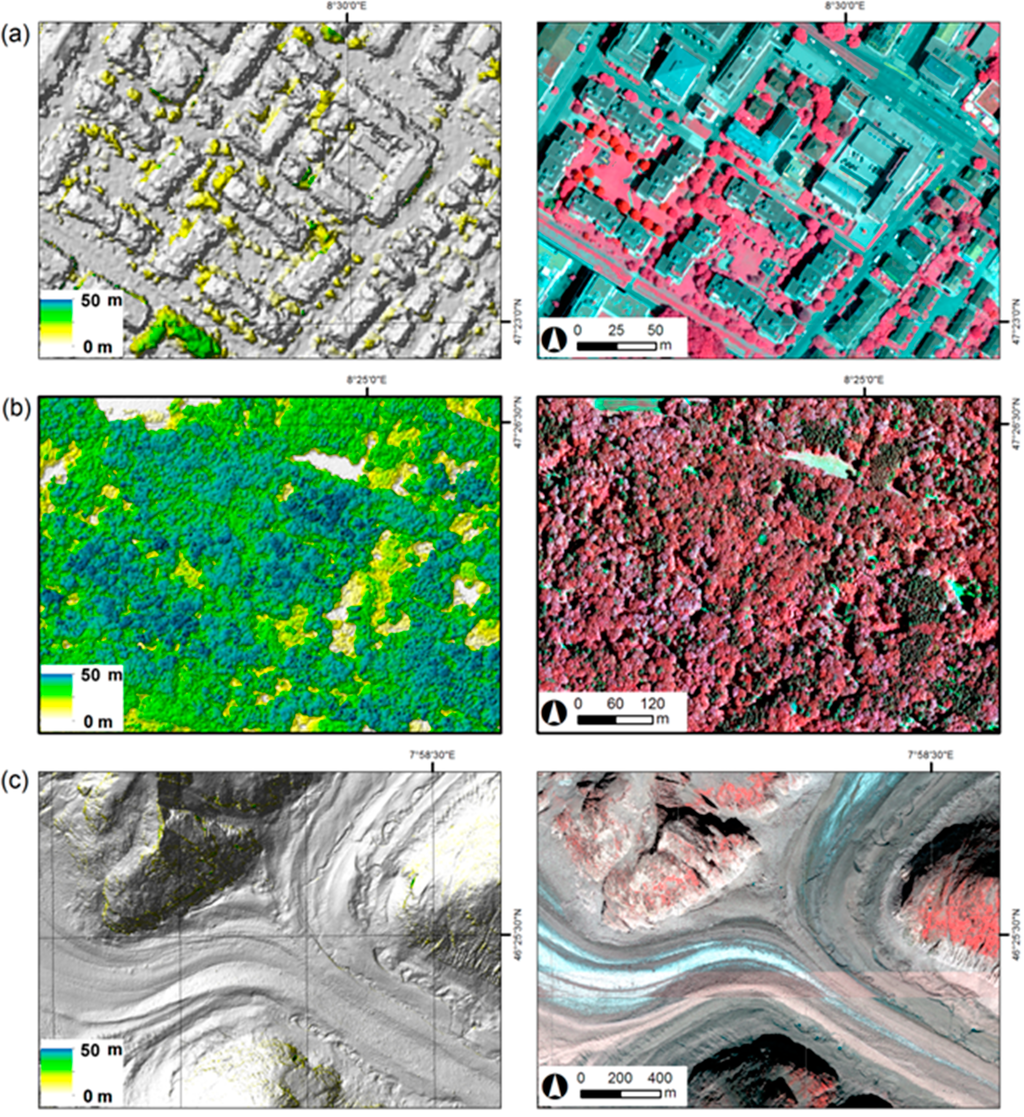
Figure 5.
Shaded relief of the generated DSM with a colour gradient for canopy height (0–50 m) on the left and the used ADS80 input image data on the right: (a) buildings in Zurich, (b) forests in the Swiss lowlands and (c) glaciers in the Valais.
To cover the entire country, a total of 166,725 image blocks were matched: 54.5% with a GSD of 0.25 m and 45.5% with a GSD of 0.5 m. The different strategies and the combination of the 1st and 2nd most nadir image stripes allowed for an overall completeness of the image matched points of 97.9% (Table 2). Already using only one strategy with one image stripe enabled an overall mean completeness of all image blocks of 94.9%. The greatest improvement was achieved while additionally processing the “ADS flat” strategy, which led to a mean gain in completeness of 1.7%. To achieve this rather minor improvement in completeness, 133,897 blocks were matched with the “ADS flat” strategy, requiring a calculation time of 98 days. For the year 2007, the gain in completeness by adding this second strategy was a very large improvement of 6.5% (see Appendix B, Table A2 and Table A3). Manual corrections of the data were done for only 0.14% of the matched blocks, most of which were done because of cloud cover. Manual correction involved visual inspection and replacement of those results showing a high proportion of errors with data from earlier years.
The mean calculation time per image block was 16 min for one strategy. In our study, the matching process, distributed to 16 virtual PCs, was completed within approximately 320 days (including ~10% for database updates and network maintenance). Thus, within two months, the annually acquired image data for one sixth of the country (~7000 km2) can be processed and an updated CHM can be provided. Abandoning the second strategy would reduce the calculation time from 320 to 218 days, corresponding to a reduction of 32%.
Table 2.
Gain in completeness of matched points with the different strategies and image stripes used.
| Strategy | Number of Blocks | Mean Cumulative Completeness | Mean Gain in Completeness |
|---|---|---|---|
| Strategy 1 “ADS steep” 1st most nadir image (S11) | 160,407 | 94.9% | - |
| Strategy 2 “ADS flat” 1st most nadir image (S12) | 133,879 | 96.6% | 1.7% |
| Strategy 1 “ADS steep” 2nd most nadir image (S21) | 69,969 | 97.8% | 1.2% |
| Strategy 2 “ADS flat” 2nd most nadir image (S22) | 38,166 | 97.9% | 0.1% |
3.2. Accuracies of Digital Surface Model (DSM)
3.2.1. Topographic Survey Points
Within the national triangulation network, all 198 topographic survey points could be successfully used for accuracy assessment (Table 3). The median deviations, with values of 0.07 and −0.11 m, are well below one pixel and result in a normalized median absolute deviation (NMAD) of little more than one pixel. The positive median values in the case of 0.25 m GSD indicate lower elevation values of the topographic survey points in comparison to those of the digital surface model. For images with 0.5 m GSD, the opposite was the case.
Table 3.
Vertical accuracy measurements of the digital surface model based on 198 swisstopo topographic survey points. Differences were calculated by subtracting the elevation values of the topographic survey points from those from the digital surface model. A threshold value of ±3 × RMSE was applied for outlier exclusion.
| GSD [m] | Sample Size | Sample Size No Outliers | Median [m] | NMAD [m] | Quantile 68% [m] | Quantile 95% [m] | RMSE [m] | RMSE No Outliers [m] |
|---|---|---|---|---|---|---|---|---|
| 0.25 | 164 | 161 | 0.07 | 0.29 | 0.20 | 0.74 | 0.38 | 0.34 |
| 0.50 | 34 | 34 | –0.11 | 0.64 | 0.13 | 1.08 | 0.81 | 0.81 |
3.2.2. Stereo Measurements of the National Forest Inventory
The combination of the DSM and the stereo measurement data enabled an agreement assessment over various land cover types (Table 4). The lowest median and NMAD values were found for sealed surfaces. NMAD values below 1.5 m were found for all land cover classes except forested areas. Forest trees were the most difficult ones to model, as indicated by high NMAD values varying between 1.76 and 3.94 m. Additionally, the influence of the nadir distance on accuracy measurements was evaluated and median errors were found to rise slightly with the increase in distance to the nadir line of the image stripe. This result was independent of the land cover type. Glaciers, firns and snow in the high mountain areas were only covered with images of 0.5 m GSD.
Table 4.
Vertical agreement measurements of the digital surface model per land cover type based on stereo measurements. Differences were calculated by subtracting the elevation values of the stereo measurements from those of the digital surface model. A threshold value of ±3 × RMSE was applied for outlier exclusion.
| Land Cover | GSD [m] | Sample Size | Sample Size No Outliers | Median [m] | NMAD [m] | Quantile 68% [m] | Quantile 95% [m] | RMSE [m] | RMSE no Outliers [m] |
|---|---|---|---|---|---|---|---|---|---|
| Coniferous tree | 0.25 | 24,996 | 24,925 | −0.08 | 1.76 | 0.84 | 7.06 | 9.01 | 4.21 |
| 0.50 | 7594 | 7422 | −0.34 | 2.39 | 0.77 | 6.50 | 4.55 | 3.34 | |
| Deciduous tree | 0.25 | 13,211 | 12,864 | 0.16 | 2.95 | 1.66 | 8.87 | 5.94 | 4.57 |
| 0.50 | 11,076 | 10,854 | −0.79 | 3.94 | 1.00 | 9.07 | 6.56 | 5.54 | |
| Deciduous conifer (Larch) | 0.25 | 201 | 196 | 0.45 | 2.64 | 1.65 | 8.90 | 4.48 | 3.40 |
| 0.50 | 878 | 860 | −0.80 | 3.68 | 0.94 | 7.92 | 5.68 | 4.75 | |
| Shrub | 0.25 | 444 | 437 | −0.33 | 0.84 | 0.11 | 2.06 | 1.73 | 1.18 |
| 0.50 | 2801 | 2742 | −0.22 | 1.54 | 0.50 | 4.40 | 3.21 | 2.04 | |
| Herb and grass | 0.25 | 55,736 | 55,689 | −0.13 | 0.49 | 0.10 | 2.07 | 12.52 | 3.55 |
| 0.50 | 38,429 | 37,233 | −0.25 | 0.95 | 0.20 | 6.33 | 4.09 | 1.82 | |
| Rock | 0.25 | 330 | 320 | −0.59 | 1.29 | −0.01 | 17.81 | 8.38 | 4.43 |
| 0.50 | 10,090 | 9961 | −0.74 | 1.44 | −0.11 | 3.27 | 5.46 | 2.84 | |
| Sand, stones & visible earth | 0.25 | 2060 | 2046 | 0.05 | 1.11 | 0.80 | 25.59 | 36.09 | 9.81 |
| 0.50 | 14,273 | 14,247 | −0.51 | 0.89 | −0.08 | 1.88 | 22.03 | 3.09 | |
| Sealed surface | 0.25 | 5451 | 5445 | −0.04 | 0.52 | 0.22 | 3.05 | 13.41 | 2.64 |
| 0.50 | 958 | 936 | 0.05 | 0.77 | 0.41 | 4.67 | 2.51 | 1.50 | |
| Building | 0.25 | 2925 | 2919 | 0.12 | 0.83 | 0.52 | 2.61 | 8.40 | 2.12 |
| 0.50 | 366 | 359 | −0.24 | 1.12 | 0.29 | 2.16 | 3.94 | 2.11 | |
| Glaciers, firns & snow | 0.25 | - | - | - | - | - | - | - | - |
| 0.50 | 3965 | 3880 | −0.53 | 1.53 | 0.13 | 3.01 | 2.70 | 2.11 |
We found increasing NMAD values with increasing slope inclination for both categories 0.25 and 0.5 m GSD (Table 5). The same trend was found for the RMSE without outliers and the quantile values. Contrary to the effects of slope inclination, different aspects were found to have no influence on the accuracy of the digital surface model (Appendix C, Table A4).
Table 5.
Vertical agreement measurements of the digital surface model based on stereo measurements covering five slope classes. Differences were calculated by subtracting the elevation values of the stereo measurements from the values of the digital surface model. A threshold value of ±3 × RMSE was applied for outlier exclusion.
| Slope [°] | GSD [m] | Sample Size | Sample Size no Outliers | Median [m] | NMAD [m] | Quantile 68% [m] | Quantile 95% [m] | RMSE [m] | RMSE no Outliers [m] |
|---|---|---|---|---|---|---|---|---|---|
| ≤10 | 0.25 | 63,232 | 63,165 | −0.16 | 0.67 | 0.18 | 5.10 | 13.70 | 3.28 |
| 0.50 | 7944 | 7923 | −0.44 | 0.90 | −0.04 | 1.94 | 29.27 | 2.31 | |
| >10 & ≤20 | 0.25 | 24,319 | 23,587 | −0.17 | 1.30 | 0.89 | 9.48 | 4.75 | 3.10 |
| 0.50 | 17,337 | 16,872 | −0.64 | 0.96 | −0.20 | 3.73 | 3.10 | 1.85 | |
| >20 & ≤30 | 0.25 | 11,336 | 11,326 | 0.46 | 2.40 | 2.07 | 12.70 | 11.09 | 5.64 |
| 0.50 | 25,307 | 24,746 | −0.86 | 1.29 | −0.23 | 6.58 | 4.55 | 2.77 | |
| >30 & ≤40 | 0.25 | 4999 | 4856 | 1.17 | 3.26 | 3.02 | 15.06 | 6.50 | 5.17 |
| 0.50 | 24,098 | 23,448 | −1.01 | 1.78 | −0.02 | 7.98 | 4.43 | 3.08 | |
| >40 & ≤90 | 0.25 | 1468 | 1459 | 0.59 | 4.00 | 2.61 | 13.86 | 9.99 | 6.23 |
| 0.50 | 15,744 | 15,458 | −1.36 | 2.52 | -0.10 | 9.16 | 6.20 | 4.45 |
3.3. Forest Applications
3.3.1. Tree Height of Single Trees
The comparison of the terrestrially measured tree heights with the tree height calculated from the CHM revealed acceptable results. For areas in the lowlands with 0.25 m GSD, deciduous trees showed a lower median but a higher NMAD than coniferous trees (Table 6). In the mountains where the GSD was 0.5 m, deciduous trees still showed a lower median, but the NMAD was higher for coniferous trees. The higher quantile values for deciduous trees indicate that these trees tend to be more difficult to measure terrestrially. This result is consistent with the comparison of the 441 double tree height measurements (Appendix D, Table A5). There was a high correlation (Pearson’s r = 0.83) between the terrestrial measurements and the canopy height model values (Figure 6). There was no difference in correlation between coniferous and deciduous trees (Appendix D, Figure A1). A slight difference in correlation was found between two different elevation classes (Pearson’s r = 0.72 for low elevations and Pearson’s r = 0.6 for high elevations, Appendix D, Figure A2). Outliers occurred in low numbers. They indicate cases where the forest changed between the date of the image acquisition and the terrestrial height measurement or where the digital surface model was not successful in modeling individual tree crowns.
Table 6.
Agreement of tree height calculated from the CHM with the terrestrially measured tree height. A threshold value of ±3 × RMSE was applied for outlier exclusion.
| Tree Type | GSD [m] | Sample Size | Sample Size No Outliers | Median [m] | NMAD [m] | Quantile 68% [m] | Quantile 95% [m] | RMSE [m] | RMSE [%] | RMSE No Outliers [m] | RMSE No Outliers [%] |
|---|---|---|---|---|---|---|---|---|---|---|---|
| Deciduous | 0.25 | 872 | 865 | −0.56 | 3.34 | 0.93 | 7.31 | 4.24 | 15.07 | 3.91 | 13.90 |
| 0.50 | 100 | 97 | 0.50 | 3.08 | 2.38 | 9.54 | 4.47 | 20.68 | 3.75 | 17.24 | |
| Coniferous | 0.25 | 1,562 | 1,541 | −1.86 | 2.65 | −0.54 | 4.02 | 4.30 | 14.40 | 3.63 | 12.15 |
| 0.50 | 575 | 560 | −2.54 | 3.72 | −0.81 | 4.02 | 6.28 | 27.77 | 5.02 | 19.12 |
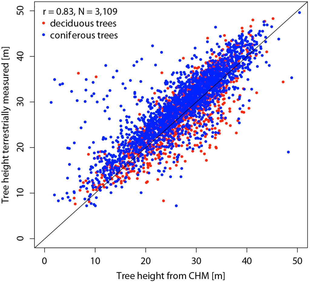
Figure 6.
Correlation between tree heights of the CHM and terrestrial tree height measurements. Total number of measurements is 3109. Tree height in the canopy height model refers to the maximum value within a buffer of 2.5 m radius around each individual tree. Tree height in the field was measured using a Vertex ultrasonic hypsometer.
3.3.2. Canopy Height at Plot Level
Good agreement between the canopy height measured terrestrially and the modeled canopy height at the plot level was found over a wide variety of forest stands (Figure 7, Appendix E, Table A8). If we focus on the different development stages of the forest stand, pole wood was found to have the highest correlation (Pearson’s r = 0.91) and mixed stands the lowest (Pearson’s r = 0.64). Regarding species mixture, the correlation was dependent on the percentage of coniferous trees within the stand, showing highest values in stands with over 90% coniferous trees (Appendix E, Figure A3, Table A6). Stand structure influenced correlation as well, showing highest values in one- and multi-layered stands and lower values in highly structured stands (Appendix E, Figure A4, Table A7).
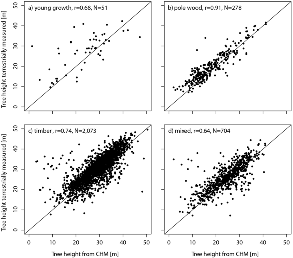
Figure 7.
Comparison of canopy height from the CHM with terrestrially measured canopy height at the NFI sample plot level. One of the four stages of stand development was assigned to each sample plot. (a) Young growth refers to regeneration areas with a medium tree height of 8 m; (b) pole wood refers to stands with a high number of stems and a mean tree height of 8–20 m; (c) the timber stage is characterized by closed stands with a mean height > 20 m; and (d) mixed refers to stands where there are different stages of stand development.
4. Discussion
4.1. Workflow for the Generation of the Models
The highlight of the nationwide digital surface generation approach presented here is the consistency of the input data and matching approaches over an entire country. The workflow used is highly automated and allows for an update of the DSM covering Switzerland every three to six years. The input image data used in this study is routinely acquired for different purposes of countrywide orthophoto production and topographic mapping. Therefore, there are limitations to the spatial and temporal resolution of the data, in comparison to projects with flight campaigns planned solely for a specific research objective. However, the great advantage of the approach lies in the opportunity for model updating that is both effective and cost-efficient. Once a digital terrain model based on ALS data is available, the photogrammetric updating of digital surface data and canopy height models using routinely acquired aerial stereo image data provides a valuable alternative to the acquisition of repeated ALS data.
In the present study, we used the SocetSet “Next-Generation Automatic Terrain Extraction” (NGATE) by BAE Systems for image matching. It enabled consistency in calculations over the different time periods and achieved a good compromise between image-matching quality and calculation time. Other software packages, such as Trimble Match-T and Leica XPro using Semi-global matching were tested in case studies. While good overall image-matching results were achieved, calculation times were at least four times as high as with NGATE implemented in SocetSet. Inaccuracies in the surface models were found for situations such as those listed by Baltsavias et al. [40], for example water surfaces, where matching was not successful due to the movement of the water surface between the two time steps of image acquisition, as well as on steep slopes or in the high mountains where whiteout was an issue.
A high level of completeness was achieved using two different matching strategies (“ADS steep” and “ADS flat”) on two pairs of imagery (1st most nadir and 2nd most nadir stripe). The combination of these strategies and input data is important to cope with the heterogeneous mosaic of different land cover types within the country. Although using one strategy applied only to one image pair would reduce the calculation time substantially (by 50%), we maintained the consistent application of the different strategies for the matching of the 1st and 2nd most nadir image stripes for each block for the whole country. The main reason was that we were striving for a very high level of completeness to allow for a broad spectrum of analysis based on this data set. The use of a second image pair was important for areas where clouds or haze led to occlusion of some image parts in the first image pair, which could be matched using the second image pair. In addition, in the case of forested areas, the use of a second image pair allowed for another view angle, for example, for oblique trees at forest edges or within canopy gaps, resulting in a substantial improvement in the image matching for those areas, even if the overall gain in completeness was not high. The combination of the two strategies was important for a successful matching of areas with low texture, such as expanse meadows, grasslands or snow areas. In these areas, the use of the second strategy enabled the matching of areas that could not be matched with the first strategy, thus leading to higher overall matching success. Especially in the case of stereo image pairs from the year 2007, where a combination of RGB and Pan images was used, this second strategy led to a substantial improvement in overall completeness.
4.2. Accuracy of the Digital Surface Model (DSM)
The accuracy of the calculated DSM is very good in the case of sealed surfaces (e.g., median difference of −0.04 m and NMAD 0.52 m for 0.25 GSD) and acceptable for most applications in forested areas (e.g., median difference of 0.16 m and NMAD of 2.95 m for deciduous trees, 0.25 GSD). A similar result for a small study area in northeast Switzerland was achieved in previous work using GPS points as reference with a median difference of 0.08 m and a NMAD of 0.21 m in flat terrain and a median difference of −1.12 m with a NMAD of 1.32 m in forested areas in comparison with stereo-measurements [41]. The deciduous tree species in this study had a greater median difference and a higher deviation than the coniferous trees. In the present study, the deviation of the values in forested areas was larger than in the above mentioned study, since calculations were made over the entire country spreading over an area of a 41,285 km2 at an altitudinal range of 200 to 4500 m a.s.l., and including a variety of forest types and tree species. There are no studies outside Switzerland based on ADS stereo aerial images to which the results of the present study could be compared. In a study of a broadleaf-dominated forest in central Europe, average differences of 0.17 m with a standard deviation of 0.29 m between the UltraCamXp image-based heights and the ALS-based heights were achieved for flat areas [15]. These values are comparable to the accuracy values of the topographic survey points in Switzerland.
To take into account variation in land cover in Switzerland, a separate analysis was performed distinguishing different land cover types based on stereo measurements. This study revealed median differences between 0.04 and 0.80 m with NMAD values ranging from 0.49 to 3.94 m. Herb and grass, and sealed areas had the highest agreement values with NMAD values of ±2 pixels for both GSD classes. Shrubs, buildings, glaciers, firn and snow, with NMAD values of ±3 pixels, showed good agreement values as well. NMAD values of up to ±5 pixels were found for areas covered by rock, stands, stones and visible earth. As expected and mentioned above, forested areas were the most difficult areas to model, achieving NMAD values of up to ±16 pixels. Looking at the influence of topography, a decrease in accuracy with increasing slope inclination was found. This is in line with a study by Bühler et al. [42] in high alpine terrain comparing ADS80 stereo image elevation values and ALS data and with the findings of Müller et al. [43] in a high mountain environment. Contrary to our expectations, no difference in accuracy was found for different aspect classes. Due to the high radiometric resolution of 12 bit, even in shadowed parts in north-facing mountainous regions, the matching was successful.
The two reference data sets used complemented each other and allowed for comprehensive assessment of the accuracy of the DSM. The topographic survey points are a completely independent data set enabling an estimation of the absolute accuracy. However, this analysis is largely dependent on the orientation of the input imagery. Small shifts in geolocation could lead to higher vertical errors. For stereo measurements, a shift in geolocation can be excluded, since these measurements were carried out on the oriented image data itself. This data set is highly suitable for the assessment of the agreement with the digital surface model over different land cover types, but cannot be used for an absolute accuracy analysis in a strict sense.
4.3. Applications within the National Forest Inventory
An important characteristic of this study is the variety of forests analyzed with regards to development stages, species mixture and stand structure. Given the very heterogeneous data set, the comparison of single tree heights and canopy height at the plot level revealed plausible results and demonstrates the potential of the canopy height model. This variation in analyzed forest types is also the reason why the RMSE values are substantially higher than some other relevant studies, for example, a Swedish study that used DMC aerial images in a coniferous forest for DSM generation, where RMSE values between 1.4 and 1.6 m were found [17], or a Finnish study based on UltraCamD images, where RMSE values ranged between 6.77% and 7.55% of tree height [19].
The accuracy of a CHM is largely dependent on the DTM used for its generation. In our case, the ALS DTM is from the years 2001–2003 and the ADS40/ADS80 images from the period 2007–2012. The time differences can be ignored, because in most areas the terrain has not changed significantly over the short period of several years. Major errors, however, can occur if there are differences in the geolocation of the DSM and the DTM, or the two models are not accurately co-registered [18]. To avoid the influence of such minor shifts in geolocation, we always used some kind of buffer while comparing different data sets for evaluation purposes.
These results show that the canopy height model is most usable for stand-wise assessment, where the focus is on estimates over the whole canopy, and the influence of individual trees is only minor. The data is less suitable for estimations of single tree parameters and estimations based on individual trees, since the spatial resolution of the input image data is too low for such specific purposes. In the framework of the Swiss National Forest Inventory, the data is used as auxiliary information to post-stratify forest areas according to canopy height for the estimation of different forest characteristics, see also [8,44]. This allows for a further reduction of estimation errors, especially when it comes to small area estimations [1,45].
5. Conclusions
For the first time, a digital surface model with a resolution of 1 × 1 m and a canopy height model covering an entire country have been calculated using an image matched point cloud with a very high completeness of matched points of 97.9%. Switzerland, at just over 41,000 km2, is a rather small country, although its mixture of different land cover types, an altitudinal gradient of 200 to 4500 m a.s.l., and the complex topography makes the country particularly interesting for this kind of research. Improvements in matching algorithms, combined with the increasing performance in terms of hardware capacity make nationwide processing of aerial stereo imagery possible, and with the highly automated workflow presented, the manual interaction during the process is reduced to a minimum. This allows for an operational generation of a 3-d data set of homogeneous data quality over a heterogeneous country, even if calculation time is still high. The agreement between the manual stereo measurements and the elevation of the calculated digital surface model at trees (NMAD below +/− 16 pixel) as well as the good correlation (Pearson’s r = 0.83, n = 3109) of terrestrially measured trees and the tree height derived from the canopy height model show the high potential of the model for country-wide forest applications.
Using routinely acquired stereo imagery, an update of models can be provided at regular intervals. For 81% of the country at least two time steps are already calculated. Initial studies for change detection are underway. This data set provides high potential to estimate changes in timber volume, gaps within the canopy or development stages of forest stands. A primary future application lies in the estimation of the extent of damage after a large windthrow, fire or insect disturbance within the forest, based on stereo imagery which is acquired immediately after the natural disturbance event.
Acknowledgments
This study was carried out within the framework of the Swiss National Forest Inventory (NFI), a cooperation between the Swiss Federal Research Institute WSL and the Swiss Federal Office for the Environment FOEN. We are grateful to Lucinda Laranjeiro and Daniel Uebersax for the stereo-measurements on the ADS40/ADS80 images. We thank Mauro Marty for valuable comments on an earlier version of the manuscript. We acknowledge Curtis Gautschi and Bronwyn Price for the linguistic revision of the text. We want to thank the anonymous reviewers for helping to improve the manuscript.
Author Contributions
Christian Ginzler designed research and generated models; Martina L. Hobi and Christian Ginzler analyzed data, calculated statistics and wrote the manuscript.
Appendix
A. Technical Details of the Sensor
Table A1.
Technical details of the Advanced Digital Sensors (ADS) used.
| Parameter | ADS40-SH40 | ADS40-SH52 | ADS80-SH82 |
|---|---|---|---|
| Time of operation | until 2007 | 2008–present | 2009–present |
| Sensor | Three-line CCD scanner | Three-line CCD scanner | Three-line CCD scanner |
| Dynamic range of the CCD | 12 bit | 12 bit | 12 bit |
| Spectral bands [nm] | Panchromatic 465–680 | Panchromatic 465–680 | Panchromatic 465–680 |
| Blue 430–490 | Blue 428–492 | Blue 428–492 | |
| Green 535–585 | Green 533–587 | Green 533–587 | |
| Red 610–660 | Red 608–662 | Red 608–662 | |
| Near infrared 835–885 | Near infrared 833–887 | Near infrared 833–887 | |
| CCD elements | 8 CCD lines with 12,000 pixel each | 12 CCD lines with 12,000 pixel each | 12 CCD lines with 12,000 pixel each |
| Pixel size [µm] | 6.5 | 6.5 | 6.5 |
| Focal plate configuration | Pan F28° NIR F18° Green F16° Red F14° Blue N0° Green N0° Red N0° Pan B14° | Pan F27° | Pan F27° |
| Pan F02° | Pan F02° | ||
| Blue N0° | Blue N0° | ||
| Green N0° | Green N0° | ||
| Red N0° | Red N0° | ||
| NIR N0° | NIR N0° | ||
| Pan B14° | Pan B14° | ||
| Blue B16° | Blue B16° | ||
| Green B16° | Green B16° | ||
| Red B16° | Red B16° | ||
| NIR B16° | NIR B16° |
B. Completeness
For all image data sets of the different acquisition years, completeness is over 90% after the first image strategy used for each block. In the case of the year 2007, values are slightly lower in comparison to other years, which can be related to the use of a different combination of spectral bands (Table A1). The greatest gain in completeness was achieved by using the second strategy on the same image stripe (Table A2 and Table A3). A similar improvement was achieved when using a second image stripe and only a minimal gain in completeness was found by using the second strategy on the second image stripe. The overall gain in completeness using the different strategies and two image stripes was 3% in the years from 2008 to 2012 and 8.1% for the year 2007.
Table A2.
Mean completeness values of the blocks using different strategies for the different years of image acquisition (S11: 1st nadir stripe/“ADS steep”, S12: 1st nadir stripe/“ADS flat”, S21: 2nd nadir stripe/“ADS steep”, S22: 2nd nadir stripe/“ADS flat”).
| Year of Data Acquisition | Completeness S11 [%] | Completeness S12 [%] | Completeness S21 [%] | Completeness S22 [%] |
|---|---|---|---|---|
| 2007 | 90.2 | 96.7 | 98.0 | 98.3 |
| 2008 | 94.4 | 96.0 | 97.6 | 97.7 |
| 2009 | 94.9 | 96.2 | 97.6 | 97.7 |
| 2010 | 94.9 | 96.6 | 97.8 | 97.9 |
| 2011 | 95.2 | 96.4 | 97.6 | 97.7 |
| 2012 | 94.5 | 96.3 | 97.7 | 97.9 |
Table A3.
Gain in completeness with the different strategies and image stripes used. Comparison of the year 2007 where a combination of Pan and RGB was used and the years 2008–2012 where matching was based on CIR images (S11: 1st nadir stripe/“ADS steep”, S12: 1st nadir stripe/“ADS flat”, S21: 2nd nadir stripe/“ADS steep”, S22: 2nd nadir stripe/“ADS flat”).
| Year of Data Acquisition | Gain in Completeness S11‒S12 [%] | Gain in Completeness S12‒S21 [%] | Gain in Completeness S21‒S22 [%] | Gain in Completeness S11‒S22 [%] |
|---|---|---|---|---|
| 2007 | 6.5 | 1.3 | 0.3 | 8.1 |
| 2008–2012 | 1.5 | 1.4 | 0.1 | 3.0 |
C. Accuracy Assessment of DSM
Other than the slope, aspect was found to have only a minor influence on the accuracy of the DSM (Table A4). One could expect that northern exposed slopes affected by shadow effects would show larger errors. This, however, did not occur, indicating that the 12 bit ADS40/ADS80 data allow for good image matching even in shadowy areas.
Table A4.
Vertical agreement measurements of the digital surface model based on stereo measurements distinguishing eight aspect classes. Differences are calculated by subtracting the elevation values of the stereo measurements from the digital surface model values. A threshold value of ±3 × RMSE was applied for outlier exclusion.
| Exposure | GSD [m] | Sample Size | Sample Size No Outliers | Median [m] | NMAD [m] | Quantile 68% [m] | Quantile 95% [m] | RMSE [m] | RMSE no Outliers [m] |
|---|---|---|---|---|---|---|---|---|---|
| N | 0.25 | 15,622 | 15,575 | −0.07 | 0.87 | 0.36 | 8.66 | 9.81 | 9.81 |
| 0.50 | 12,179 | 12,159 | −0.47 | 1.35 | 0.14 | 7.44 | 10.92 | 4.58 | |
| NE | 0.25 | 6,673 | 6,492 | −0.07 | 0.74 | 0.26 | 5.93 | 4.20 | 3.83 |
| 0.50 | 5,189 | 5,047 | −0.51 | 1.39 | 0.10 | 7.26 | 4.99 | 3.03 | |
| E | 0.25 | 25,069 | 24,964 | −0.09 | 0.79 | 0.26 | 5.44 | 8.48 | 8.47 |
| 0.50 | 22,802 | 22,184 | −0.39 | 1.16 | 0.12 | 4.19 | 3.95 | 2.31 | |
| SE | 0.25 | 15,272 | 15,229 | −0.10 | 0.8 | 0.24 | 5.18 | 8.96 | 8.95 |
| 0.50 | 11,578 | 11,378 | −0.25 | 1.23 | 0.30 | 3.97 | 4.81 | 2.67 | |
| S | 0.25 | 9291 | 9040 | −0.14 | 0.73 | 0.20 | 5.56 | 4.22 | 3.95 |
| 0.50 | 9509 | 9252 | −0.25 | 1.23 | 0.26 | 3.79 | 3.67 | 2.21 | |
| SW | 0.25 | 9,727 | 9713 | −0.15 | 0.77 | 0.20 | 5.87 | 11.50 | 11.50 |
| 0.50 | 10,556 | 10,339 | −0.35 | 1.23 | 0.22 | 5.40 | 4.45 | 2.58 | |
| W | 0.25 | 13,957 | 13,612 | −0.09 | 0.79 | 0.26 | 7.55 | 5.77 | 5.00 |
| 0.50 | 12,671 | 12,649 | −0.43 | 1.3 | 0.16 | 8.69 | 21.57 | 4.63 | |
| NW | 0.25 | 9602 | 9578 | −0.07 | 0.85 | 0.31 | 8.16 | 22.17 | 22.20 |
| 0.50 | 5946 | 5751 | −0.42 | 1.44 | 0.24 | 10.12 | 5.31 | 3.30 |
D. Comparison of Individual Tree Height Measurements
We found no difference in the correlation between tree height extracted from the CHM and terrestrial height measurements when distinguishing between coniferous and deciduous trees (Figure A1). However, as expected, the correlation was higher for trees in the lowlands than for trees at higher elevations (Figure A2).
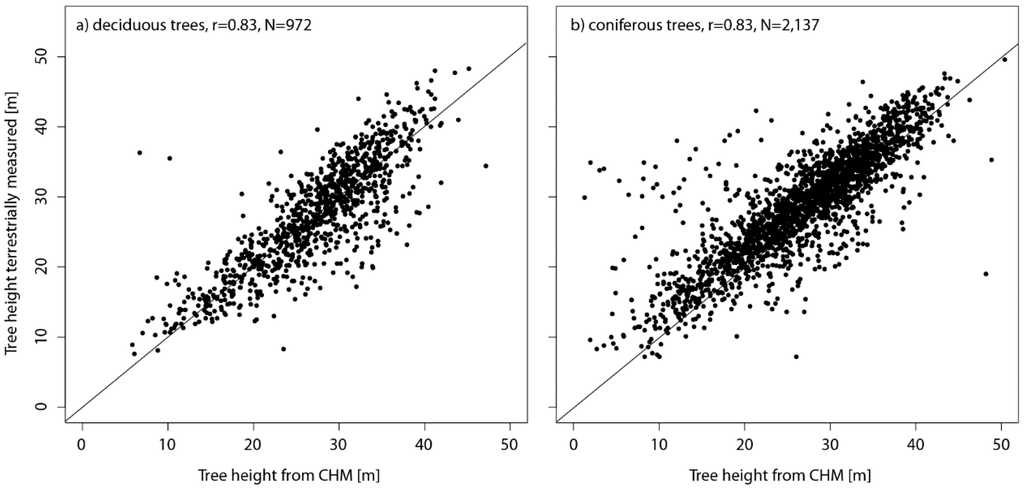
Figure A1.
Correlation of tree height extracted from the CHM with terrestrial tree height measurements distinguishing between (a) deciduous and (b) coniferous trees. The total number of measurements was 3109. Tree height in the canopy height model refers to the maximum value within a buffer of 5 m diameter around each individual tree. Tree height in the field was measured using a Vertex ultrasonic hypsometer.
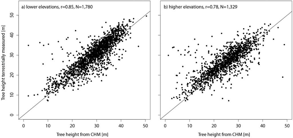
Figure A2.
Correlation between tree height extracted from the CHM and terrestrial tree height measurements distinguishing between (a) lower and (b) higher elevations. Total number of measurements was 3109. Tree height in the canopy height model refers to the maximum value within a buffer of 5 m diameter around each individual tree. Tree height in the field was measured using a Vertex ultrasonic hypsometer.
Double measurements of trees within the Swiss NFI were used to estimate how these differences in correlations are influenced by the accuracy of tree height measurement in the field (Table A5). As expected, coniferous trees could be measured more accurately than deciduous trees.
Table A5.
Comparison of double measurements of the heights of 441 trees within the Swiss NFI to estimate measurement error. A threshold value of ±3 × RMSE was applied for outlier exclusion.
| Tree Type | Sample Size | Sample Size No Outliers | Median [m] | NMAD [m] | Quantile 68% [m] | Quantile 95% [m] | RMSE [m] | RMSE No Outliers [m] |
|---|---|---|---|---|---|---|---|---|
| Deciduous | 117 | 116 | −0.10 | 1.93 | 0.72 | 3.28 | 2.42 | 2.28 |
| Coniferous | 324 | 320 | −0.15 | 1.26 | 0.50 | 3.27 | 1.72 | 1.55 |
E. Canopy Height at the Plot Level
At the plot level, species mixture had some influence on the agreement of tree height in the CHM and the terrestrially measured tree heights (Figure A3). The best correlation was found for stands dominated by over 90% coniferous trees. Stand structure influenced the correlation as well (Figure A4). Stands with clear layering could be better mapped than stands with a high variation of canopy height at the plot level.
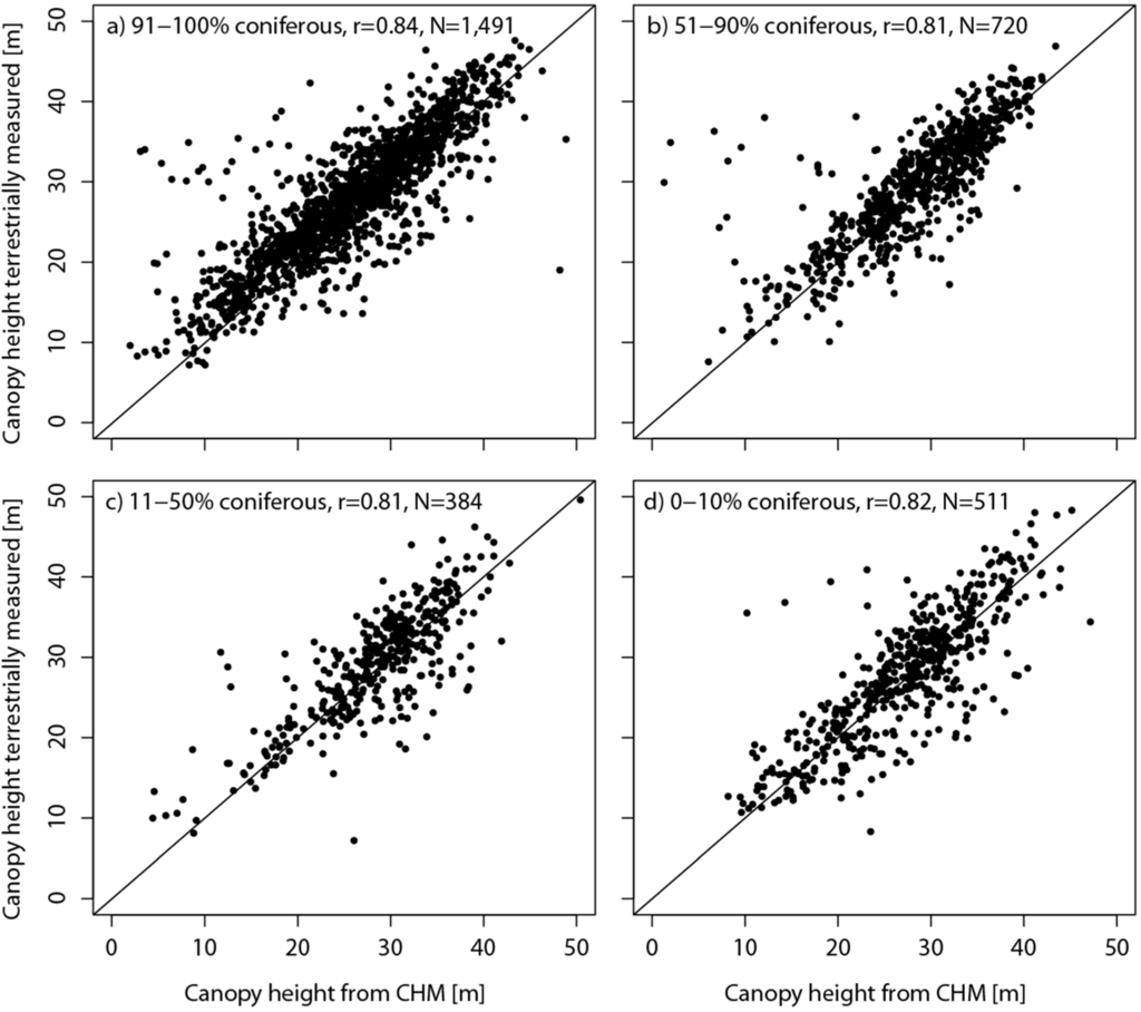
Figure A3.
Comparison of canopy height of the CHM with terrestrially measured canopy height at the sample plot level of the NFI. One of the four species mixture classes (a–d) depending on the percentage of intermixed coniferous trees was assigned to each sample plot.
Table A6.
Agreement of canopy height calculated from the CHM with the terrestrially measured canopy height according to species mixture. A threshold value of ±3 × RMSE was applied for outlier exclusion.
| Percentage Coniferous | GSD [m] | Sample Size | Sample Size No Outliers | Median [m] | NMAD [m] | Quantile 68% [m] | Quantile 95% [m] | RMSE [m] | RMSE No Outliers [m] |
|---|---|---|---|---|---|---|---|---|---|
| 91%–100% | 0.25 | 963 | 954 | −1.96 | 2.80 | −0.53 | 4.76 | 4.04 | 3.72 |
| 0.50 | 528 | 515 | −2.46 | 3.85 | −0.81 | 4.02 | 6.24 | 4.98 | |
| 51%–90% | 0.25 | 669 | 657 | −1.35 | 2.55 | −0.18 | 4.49 | 4.52 | 3.38 |
| 0.50 | 51 | 49 | −0.97 | 3.02 | 0.24 | 3.47 | 4.37 | 3.23 | |
| 11%–50% | 0.25 | 353 | 349 | −0.97 | 3.13 | 0.46 | 7.08 | 4.27 | 3.95 |
| 0.50 | 31 | 30 | −0.88 | 3.28 | 1.20 | 10.58 | 5.48 | 4.38 | |
| 0%–10% | 0.25 | 448 | 445 | −0.94 | 3.34 | 0.65 | 7.73 | 4.42 | 4.08 |
| 0.50 | 63 | 61 | 1.28 | 3.37 | 2.92 | 11.44 | 5.90 | 4.91 |
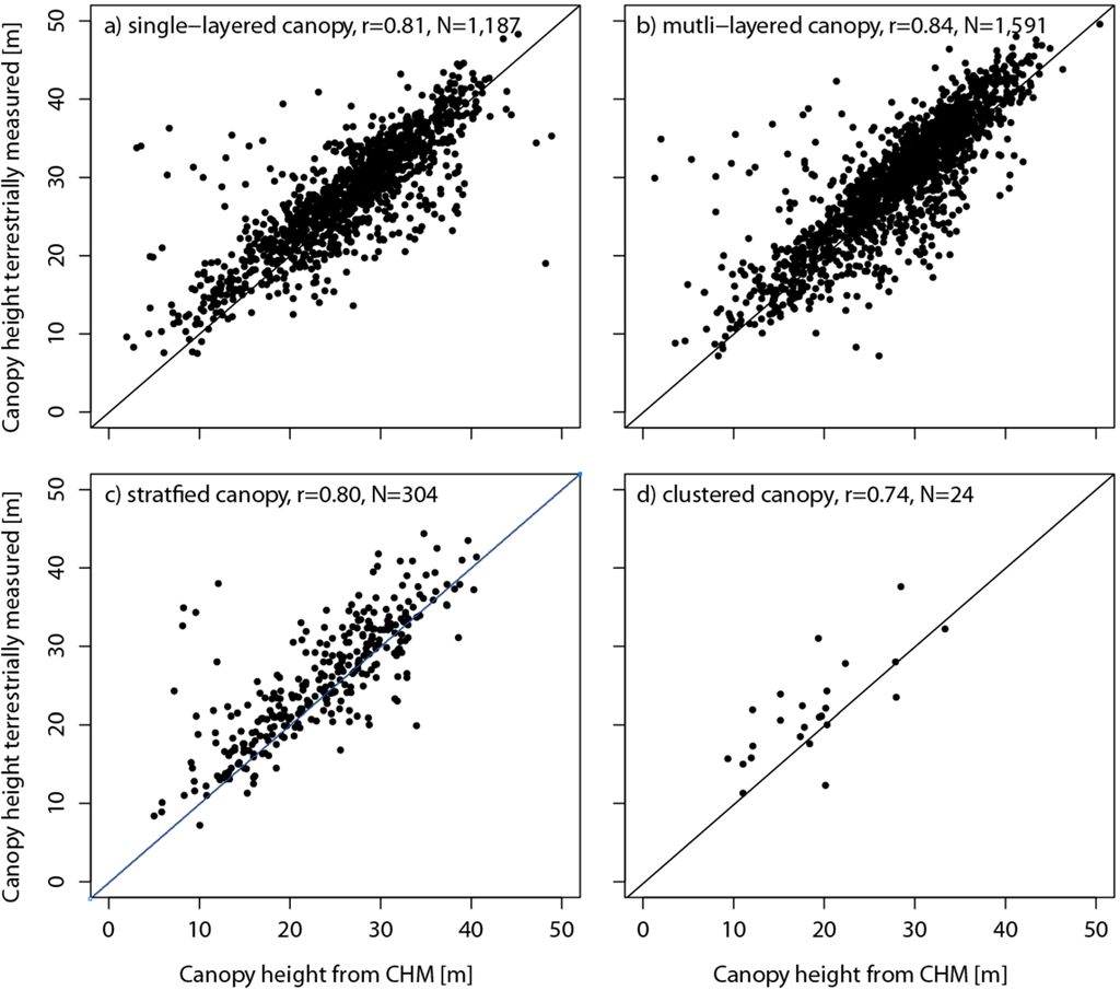
Figure A4.
Comparison of canopy height of the CHM with terrestrially measured canopy height at the sample plot level of the NFI. One of the four stand structure classes (a–d), defined by the layering and structure of the canopy was assigned to each sample plot.
Table A7.
Agreement of canopy height calculated from the CHM with the terrestrially measured canopy height according to stand structure. A threshold value of ±3 × RMSE was applied for outlier exclusion.
| Stand Structure | GSD [m] | Sample Size | Sample Size No Outliers | Median [m] | NMAD [m] | Quantile 68% [m] | Quantile 95% [m] | RMSE [m] | RMSE No Outliers [m] |
|---|---|---|---|---|---|---|---|---|---|
| Single-layered | 0.25 | 877 | 867 | −1.45 | 2.92 | −0.01 | 5.74 | 4.04 | 3.67 |
| 0.50 | 310 | 301 | −1.86 | 3.83 | −0.33 | 6.09 | 6.44 | 4.97 | |
| Multi-layered | 0.25 | 1356 | 1340 | −1.51 | 2.91 | −0.07 | 5.66 | 4.30 | 3.72 |
| 0.50 | 235 | 230 | −2.11 | 3.97 | 0.12 | 5.42 | 5.77 | 4.85 | |
| Stratified canopy | 0.25 | 192 | 188 | −1.57 | 2.89 | −0.33 | 3.31 | 5.09 | 3.88 |
| 0.50 | 112 | 110 | −1.99 | 3.90 | −0.77 | 5.03 | 5.65 | 4.83 | |
| Clustered structure | 0.25 | 8 | 8 | −0.90 | 3.53 | 0.19 | 5.38 | 6.12 | 6.12 |
| 0.50 | 16 | 16 | −3.93 | 3.28 | −1.78 | 1.95 | 4.90 | 4.90 |
Table A8.
Agreement of canopy height calculated from the CHM with the terrestrially measured canopy height according to stages of stand development. A threshold value of ±3 × RMSE was applied for outlier exclusion.
| Percentage Coniferous | GSD [m] | Sample Size | Sample Size No Outliers | Median [m] | NMAD [m] | Quantile 68% [m] | Quantile 95% [m] | RMSE [m] | RMSE No Outliers [m] |
|---|---|---|---|---|---|---|---|---|---|
| Young growth | 0.25 | 38 | 37 | −2.71 | 4.43 | −0.80 | 4.36 | 7.98 | 6.58 |
| 0.50 | 13 | 13 | −0.92 | 9.44 | 3.05 | 8.02 | 9.11 | 9.11 | |
| Pole wood | 0.25 | 221 | 219 | −1.93 | 2.62 | −0.48 | 2.36 | 3.61 | 3.23 |
| 0.50 | 57 | 57 | −1.30 | 3.28 | 0.57 | 6.33 | 3.58 | 3.58 | |
| Timber | 0.25 | 1685 | 1671 | −1.51 | 2.95 | −0.01 | 5.76 | 4.14 | 3.75 |
| 0.50 | 388 | 379 | −1.92 | 4.06 | −0.04 | 5.73 | 6.22 | 5.45 | |
| Mixed | 0.25 | 489 | 483 | −1.20 | 2.97 | 0.15 | 6.35 | 4.62 | 3.91 |
| 0.50 | 215 | 210 | −2.58 | 3.80 | −0.85 | 3.15 | 6.03 | 4.96 |
F. Sampling Scheme of the Aerial Photo-Interpretation of the Swiss National Forest Inventory
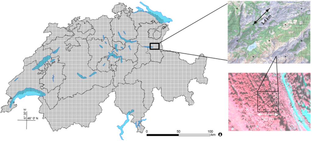
Figure A5.
Sample plots of the Swiss National Forest Inventory spaced in a regular 1.4 km grid, consisting of 25 lattice points each where height and surface cover information was measured.
Conflicts of Interest
The authors declare no conflict of interest.
References
- Massey, A.; Mandallaz, D.; Lanz, A. Integrating remote sensing and past inventory data under the new annual design of the Swiss National Forest Inventory using three-phase design-based regression estimation. Can. J. For. Res. 2014, 44, 1177–1186. [Google Scholar] [CrossRef]
- Ni, W.; Ranson, K.J.; Zhang, Z.; Sun, G. Features of point clouds synthesized from multi-view ALOS/PRISM data and comparisons with LiDAR data in forested areas. Remote Sens. Environ. 2014, 149, 47–57. [Google Scholar] [CrossRef]
- Straub, C.; Tian, J.; Seitz, R.; Reinartz, P. Assessment of Cartosat-1 and WorldView-2 stereo imagery in combination with a LiDAR-DTM for timber volume estimation in a highly structured forest in Germany. Forestry 2013, 86, 463–473. [Google Scholar] [CrossRef]
- Blackburn, G.A.; Abd Latif, Z.; Boyd, D.S. Forest disturbance and regeneration: A mosaic of discrete gap dynamics and open matrix regimes? J. Veg. Sci. 2014, 25, 1341–1354. [Google Scholar] [CrossRef]
- Vepakomma, U.; St-Onge, B.; Kneeshaw, D. Response of a boreal forest to canopy opening: Assessing vertical and lateral tree growth with multi-temporal lidar data. Ecol. Appl. 2011, 21, 99–121. [Google Scholar] [CrossRef] [PubMed]
- Camathias, L.; Bergamini, A.; Küchler, M.; Stofer, S.; Baltensweiler, A. High-resolution remote sensing data improves models of species richness. Appl. Veg. Sci. 2013, 16, 539–551. [Google Scholar] [CrossRef]
- Zellweger, F.; Braunisch, V.; Baltensweiler, A.; Bollmann, K. Remotely sensed forest structural complexity predicts multi species occurrence at the landscape scale. For. Ecol. Manag. 2013, 307, 303–312. [Google Scholar] [CrossRef]
- McRoberts, R.E.; Tomppo, E.O. Remote sensing support for national forest inventories. Remote Sens. Environ. 2007, 110, 412–419. [Google Scholar] [CrossRef]
- Gao, J. Towards accurate determination of surface height using modern geoinformatic methods: Possibilities and limitations. Prog. Phys. Geogr. 2007, 31, 591–605. [Google Scholar] [CrossRef]
- White, J.; Wulder, M.; Vastaranta, M.; Coops, N.; Pitt, D.; Woods, M. The utility of image-based point clouds for forest inventory: A comparison with airborne laser scanning. Forests 2013, 4, 518–536. [Google Scholar] [CrossRef]
- Baltsavias, E.P. A comparison between photogrammetry and laser scanning. ISPRS J. Photogram. Remote Sens. 1999, 54, 83–94. [Google Scholar] [CrossRef]
- St-Onge, B.; Vega, C.; Fournier, R.A.; Hu, Y. Mapping canopy height using a combination of digital stereo-photogrammetry and LiDAR. Int. J. Remote Sens. 2008, 29, 3343–3364. [Google Scholar] [CrossRef]
- Pitt, D.G.; Woods, M.; Penner, M. A comparison of point clouds derived from stereo imagery and airborne laser scanning for the area-based estimation of forest inventory attributes in Boreal Ontario. Can. J. Remote Sens. 2014, 40, 214–232. [Google Scholar] [CrossRef]
- Haala, N.; Hastedt, H.; Wolf, K.; Ressl, C.; Baltrusch, S. Digital photogrammetric camera evaluation—Generation of digital elevation models. Photogramm. Fernerkund. Geoinf. 2010, 2, 99–115. [Google Scholar] [CrossRef]
- Stepper, C.; Straub, C.; Pretzsch, H. Using semi-global matching point clouds to estimate growing stock at the plot and stand levels: Application for a broadleaf-dominated forest in central Europe. Can. J. For. Res. 2015, 45, 111–123. [Google Scholar] [CrossRef]
- Straub, C.; Stepper, C.; Seitz, R.; Waser, L.T. Potential of UltraCamX stereo images for estimating timber volume and basal area at the plot level in mixed European forests. Can. J. For. Res. 2013, 43, 731–741. [Google Scholar] [CrossRef]
- Bohlin, J.; Wallerman, J.; Fransson, J.E.S. Forest variable estimation using photogrammetric matching of digital aerial images in combination with a high-resolution DEM. Scand. J. For. Res. 2012, 27, 692–699. [Google Scholar] [CrossRef]
- Vastaranta, M.; Wulder, M.A.; White, J.C.; Pekkarinen, A.; Tuominen, S.; Ginzler, C.; Kankare, V.; Holopainen, M.; Hyyppä, J.; Hyyppä, H. Airborne laser scanning and digital stereo imagery measures of forest structure: Comparative results and implications to forest mapping and inventory update. Can. J. Remote Sens. 2013, 39, 382–395. [Google Scholar]
- Nurminen, K.; Karjalainen, M.; Yu, X.; Hyyppä, J.; Honkavaara, E. Performance of dense digital surface models based on image matching in the estimation of plot-level forest variables. ISPRS J. Photogram. Remote Sens. 2013, 83, 104–115. [Google Scholar] [CrossRef]
- Järnstedt, J.; Pekkarinen, A.; Tuominen, S.; Ginzler, C.; Holopainen, M.; Viitala, R. Forest variable estimation using a high-resolution digital surface model. ISPRS J. Photogram. Remote Sens. 2012, 74, 78–84. [Google Scholar] [CrossRef]
- Honkavaara, E.; Litkey, P.; Nurminen, K. Automatic storm damage detection in forests using high-altitude photogrammetric imagery. Remote Sens. 2013, 5, 1405–1424. [Google Scholar] [CrossRef]
- Hall, F.G.; Bergen, K.; Blair, J.B.; Dubayah, R.; Houghton, R.; Hurtt, G.; Kellndorfer, J.; Lefsky, M.; Ranson, J.; Saatchi, S.; et al. Characterizing 3D vegetation structure from space: Mission requirements. Remote Sens. Environ. 2011, 115, 2753–2775. [Google Scholar] [CrossRef]
- Babbar, G.; Bajaj, P.; Chawla, A.; Gogna, M. Comparative study of image matching algorithms. Int. J. Inf. Technol. Knowl. Manag. 2010, 2, 337–339. [Google Scholar]
- Swiss Federal Statistical Office (FSO). Statistical Data on Switzerland 2013; Swiss Federal Statistical Office FSO: Neuchatel, Switzerland, 2013. [Google Scholar]
- Swiss Federal Statistical Office (FSO). Land Use in Switzerland—Results of the Swiss Land Use Statistics; Swiss Federal Statistical Office FSO: Neuchatel, Switzerland, 2013. [Google Scholar]
- Brändli, U.-B. Schweizerisches Landesforstinventar: Ergebnisse der dritten Erhebung 2004–2006; Eidg. Forschungsanstalt für Wald, Schnee und Landschaft WSL: Birmensdorf, Schweiz, 2010; p. 312S. [Google Scholar]
- Swisstopo The Topographic Landscape Model TLM. Available online: http://www.swisstopo.admin.ch/internet/swisstopo/en/home/topics/geodata/TLM.html (accessed on 16 March 2015).
- Swisstopo Orthoimages. Available online: http://www.swisstopo.admin.ch/internet/swisstopo/en/home/products/images/ortho.html (accessed on 16 March 2015).
- DeVenecia, K.; Walker, S.; Zhang, B. New approaches to generating and processing high resolution elevation data with imagery. Photogramm. Week 2007, 7, 297–308. [Google Scholar]
- Zhang, L.; Gruen, A. Multi-image matching for DSM generation from IKONOS imagery. ISPRS J. Photogram. Remote Sens. 2006, 60, 195–211. [Google Scholar] [CrossRef]
- Swisstopo New National Survey LV95. Available online: http://www.swisstopo.admin.ch/internet/swisstopo/en/home/topics/survey/networks/lv95.html (accessed on 16 March 2015).
- Keller, M. Aerial Photography. In Swiss National Forest Inventory Methods and Models of the Second Assessment; Brassel, P., Lischke, H., Eds.; WSL Swiss Federal Research Institute: Birmensdorf, Switzerland, 2001. [Google Scholar]
- Mathys, L.; Ginzler, C.; Zimmermann, N.E.; Brassel, P.; Wildi, O. Sensitivity assessment on continuous landscape variables to classify a discrete forest area. For. Ecol. Manag. 2006, 229, 111–119. [Google Scholar] [CrossRef]
- Ginzler, C.; Bärtschi, H.; Bedolla, A.; Brassel, P.; Hägeli, M.; Hauser, M.; Kamphues, M.; Laranjeiro, L.; Mathys, L.; Uebersax, D.; et al. Luftbildinterpretation LFI3—Interpretationsanleitung zum dritten Landesforstinventar; Eidg. Forschungsanstalt für Wald, Schnee und Landschaft WSL: Birmensdorf, Schweiz, 2005. [Google Scholar]
- Oksanen, J.; Sarjakoski, T. Uncovering the statistical and spatial characteristics of fine toposcale DEM error. Int. J. Geogr. Inf. Sci. 2006, 20, 345–369. [Google Scholar] [CrossRef]
- Chen, C.F.; Fan, Z.M.; Yue, T.X.; Dai, H.L. A robust estimator for the accuracy assessment of remote-sensing-derived DEMs. Int. J. Remote Sens. 2012, 33, 2482–2497. [Google Scholar] [CrossRef]
- Höhle, J.; Höhle, M. Accuracy assessment of digital elevation models by means of robust statistical methods. ISPRS J. Photogram. Remote Sens. 2009, 64, 398–406. [Google Scholar] [CrossRef]
- R Development Core Team. R: A Language and Environment for Statistical Computing; R Foundation for Statistical computing: Vienna, Austria, 2008. [Google Scholar]
- Artuso, R.; Bovet, S.; Streilein, A. Practical methods for the verification of countrywide terrain and surface models. In Proceedings of the ISPRS Working Group III/3 Workshop XXXIV–3/W13. 3-D reconstruction from airborne laserscanner and InSAR data, Dresden, Germany, 8–10 October 2003.
- Baltsavias, E.; Gruen, A.; Eisenbeiss, H.; Zhang, L.; Waser, L.T. High-quality image matching and automated generation of 3D tree models. Int. J. Remote Sens. 2008, 29, 1243–1259. [Google Scholar] [CrossRef]
- Hobi, M.L.; Ginzler, C. Accuracy assessment of digital surface models based on WorldView-2 and ADS80 stereo remote sensing data. Sensors 2012, 12, 6347–6368. [Google Scholar] [CrossRef] [PubMed]
- Bühler, Y.; Marty, M.; Ginzler, C. High resolution DEM generation in high-alpine terrain using airborne remote sensing techniques. Trans. GIS 2012, 16, 635–647. [Google Scholar] [CrossRef]
- Müller, J.; Gärtner-Roer, I.; Thee, P.; Ginzler, C. Accuracy assessment of airborne photogrammetrically derived high-resolution digital elevation models in a high mountain environment. ISPRS J. Photogram. Remote Sens. 2014, 98, 58–69. [Google Scholar] [CrossRef]
- McRoberts, R.E.; Cohen, W.B.; Naesset, E.; Stehman, S.V.; Tomppo, E.O. Using remotely sensed data to construct and assess forest attribute maps and related spatial products. Scand. J. For. Res. 2010, 25, 340–367. [Google Scholar] [CrossRef]
- Magnussen, S.; Mandallaz, D.; Breidenbach, J.; Lanz, A.; Ginzler, C. National forest inventories in the service of small area estimation of stem volume. Can. J. For. Res. 2014, 44, 1079–1090. [Google Scholar] [CrossRef]
© 2015 by the authors; licensee MDPI, Basel, Switzerland. This article is an open access article distributed under the terms and conditions of the Creative Commons Attribution license (http://creativecommons.org/licenses/by/4.0/).