Abstract
Although shrublands, savannas and grasslands account for 37% of the world’s terrestrial area, not many studies have analysed the role of these ecosystems in the global carbon cycle at a regional scale. The MODIS Gross Primary Production (GPP) product is used here to help bridge this gap. In this study, the agreement between the MODIS GPP product (GPPm) and the GPP Eddy Covariance tower data (GPPec) was tested for six different sites in temperate and dry climatic regions (three grasslands, two shrublands and one evergreen forest). Results of this study show that for the non-forest sites in water-limited areas, GPPm is well correlated with GPPec at annual scales (r2 = 0.77, n = 12; SEE = 149.26 g C∙m−2∙year−1), although it tends to overestimate GPP and it is less accurate in the sites with permanent water restrictions. The use of biome-specific models based on precipitation measurements at a finer spatial resolution than the Data Assimilation Office (DAO) values can increase the accuracy of these estimations. The seasonal dynamics and the beginning and end of the growing season were well captured by GPPm for the sites where (i) the productivity was low throughout the year or (ii) the changes in the flux trend were abrupt, usually due to the restrictions in water availability. The agreement between GPPec and GPPm in non-forested sites was lower on a weekly basis than at an annual scale (0.44 ≤ r2 ≤ 0.49), but these results were improved by including meteorological data at a finer spatial scale, and soil water content and temperature measurements in the model developed to predict GPPec (0.52 ≤ r2 ≤ 0.65).
1. Introduction
Although shrublands, savannas and grasslands account for 37% of the world’s terrestrial area, many studies have been conducted to estimate how forests contribute to the global carbon cycle [1,2,3,4,5,6,7,8], but not many monitor the implications of grasslands/shrublands on the carbon cycle at a large scale [9,10]. Monitoring these non-forested ecosystems in dry areas is important since they are very sensitive to changes in water availability [11] and because they have been suggested as potential candidate areas for major carbon storage efforts [12]. Some of these areas were recorded as carbon sinks, while during years of drought the same areas were carbon sources [13], so long-term measurements at the regional scale are essential for examining the seasonal and inter-annual variability of C fluxes [14].
The net ecosystem exchange (NEE) is the CO2 exchange between the atmosphere and the whole terrestrial ecosystem [15] and it can be decomposed into two terms: gross primary production (GPP) and total ecosystem respiration (Re) [16]. While NEE is directly measurable using Eddy covariance (EC) flux towers [17], it is not possible to obtain direct, integrated observations of either GPP or Re, because these processes represent a multitude of responses by a combination of autotrophic and heterotrophic organisms [15]. However, the GPP estimates from EC towers (GPPec) only represent fluxes at the tower footprint scale (between one hundred metres and several kilometres) [18], and therefore, the estimation of GPP at regional scale can only be made by using ecosystem models (e.g., [19,20] and/or remotely sensed data (e.g., [2,21,22,23]).
Although in the past satellite sensors such as the Advanced Very High Resolution Radiometer (AVHRR) aboard the NOAA satellite and the VEGETATION (VGT) sensor aboard the SPOT satellite have been used to estimate carbon fluxes [24,25,26], the most frequently used remote sensing data source to monitor the C cycle at regional or global scale is the Moderate Resolution Imaging Spectroradiometer (MODIS) (e.g., [18,21,22,27]). MODIS estimates of GPP (GPPm) are derived from the MOD17 algorithm, which uses input data from three sources: the eight class 1 km MODIS land cover classification [27], the global scale meteorology obtained from NASA’s Data Assimilation Office GEOS-4 global climate model [28], and the fAPAR (fraction of Absorbed Photosynthetically Active Radiation).
The utility and applicability of GPPm is linked to its validation, which is challenging because of scaling issues and also the logistical constraints of measuring NPP in the field [16]. Site specific studies such as [2,29,30,31] as well as the two most comprehensive validation projects (the Bigfoot [6] and the AmeriFlux [8,13]) focused on the inter-annual variation of GPPm in forested biomes in non-water deficient areas [13,16,18]. The lack of research focused on GPPm in grasslands was partially filled by [32], which analysed the agreement with GPPec on an eight-day interval on five grasslands in three dry and two continental areas. They found that GPPm agreed well with tower data for three sites (r > 0.80), but did not capture the seasonal dynamics for the two other sites, and they recommended to extend this work to other grassland ecoregions and ecosystems. Therefore, there is a deficit of studies where GPPm is validated at an annual and at an intra-annual scale on non-forested biomes in water limited areas, since the previous similar works [32] only considered the performance of GPP in one biome (grasslands) and at one temporal scale (weekly). There is also a need for operational methods that can increase the accuracy of the GPPm estimations in these biomes, such as identifying the variables which can reduce the uncertainty in the prediction models. The aim of this work is to cover that gap.
The specific research objectives are to: (i) determine the suitability of the MODIS GPP product to estimate annual GPP and temporal dynamics of the carbon fluxes at eight-day intervals, (ii) determine the variables which improve the correlation between GPPm and GPPec for shrublands and grasslands in water deficient areas using EC carbon flux tower data.
2. Materials and Methods
2.1. Study Area
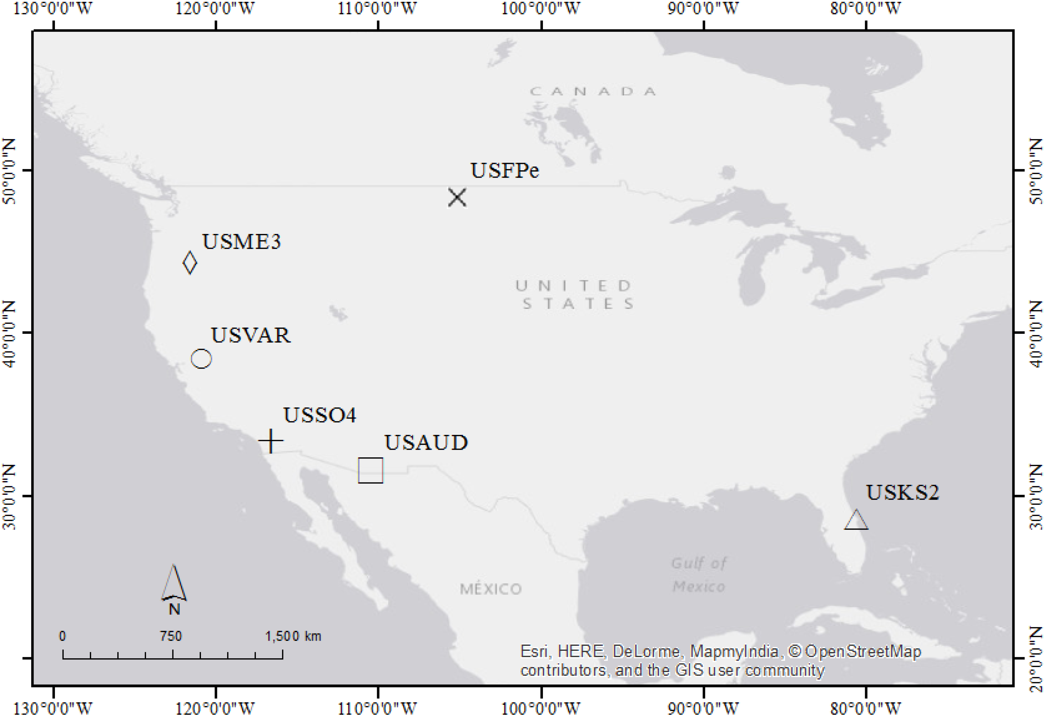
Six sites (three grasslands, two shrublands and one evergreen forest) located in temperate and dry climatic regions were selected to carry out this work, corresponding to the location of six EC carbon flux towers (Figure 1, Table 1). The time series of available data for these sites were long and the quality of the corresponding MODIS data was flagged as high in the image quality reports.
Four of these sites (USAUD, USFPe, USVAR, USSO4) are located in water deficient areas (according to the Köppen-Geiger classification system: Bsh, Bsk, Csa, [33]). One site (USKS2) is located in a non-water deficient area, in order to compare the results between water limited and non-water limited sites. In addition, one extra site (USME3) was located in an evergreen needle leaf forested area in a Mediterranean climatic region (water deficient during summer). This last site was selected to compare the results obtained for the grasslands/shrublands sites with a forested site.

Table 1.
Characteristics of the data set. Notes: ID (Fluxnet site code), Elev. (elevation in metres above sea level), IGBP (MODIS International Geosphere-Biosphere Programme (IGBP) classification): GRA: grasslands, CSH: Closed Shrublands, ENF: Evergreen Needleleaf Forest, CLIM (climatic classification according to Köppen-Geiger classification system [33]: Bsh: Hot semi-arid, Bsk: Cold semi-arid, Csa: Mediterranean, Csb: Cool-summer Mediterranean, Cfa: humid subtropical), EC data (data available from the EC Tower), EC used data (data used from the EC Tower).
| Site Name | ID | Latitude (º) | Longitude (º) | Elev. (m) | IGBP | CLIM | EC Data | EC Data Used |
|---|---|---|---|---|---|---|---|---|
| Audubon | USAUD | 31.59 | −110.51 | 1469.0 | GRA | Bsh | 2002–2005 | 2003, 2004, 2005 |
| Fort Peck | USFPe | 48.30 | −105.10 | 634.0 | GRA | Bsk | 2000–2006 | 2004, 2005, 2006 |
| Vaira Ranch-Ione | USVAR | 38.41 | −120.95 | 129.0 | GRA | Csa | 2001–2006 | 2004, 2005, 2006 |
| Kennedy Space Center (scrub oak) | USKS2 | 28.60 | −80.67 | 3.0 | CSH | Cfa | 2000–2006 | 2005, 2006 |
| Sky Oaks-new stand | USSO4 | 33.38 | −116.64 | 1429.0 | CSH | Csa | 2004–2006 | 2004, 2005, 2006 |
| Metolius-second young aged pine | USME3 | 44.31 | −121.60 | 1005.0 | ENF | Csb | 2004–2005 | 2004, 2005 |
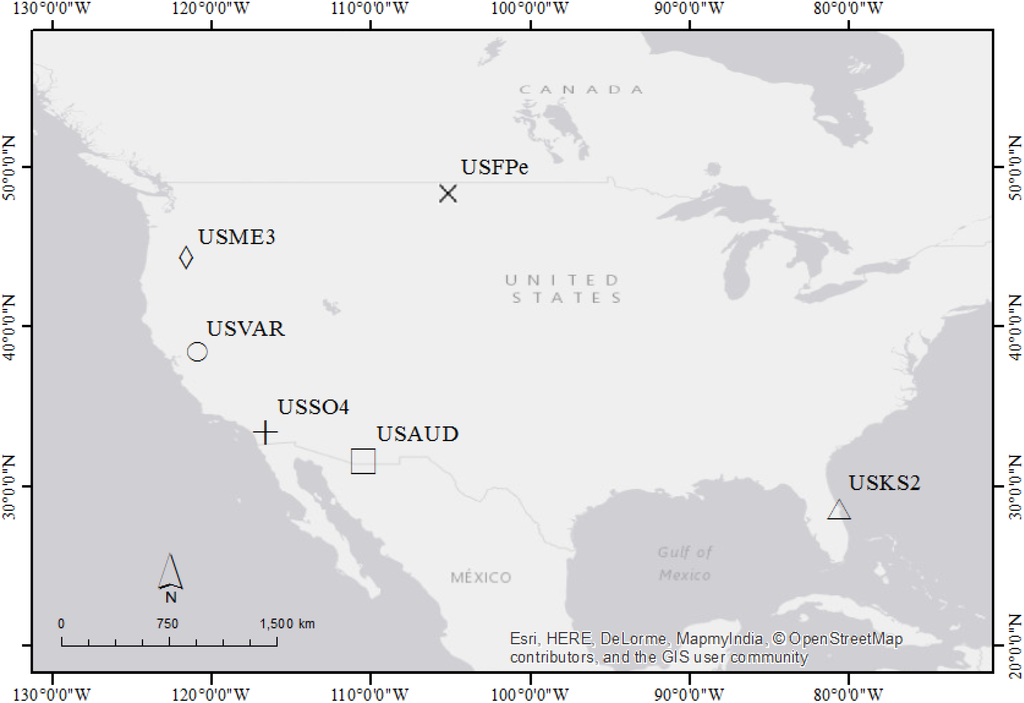
Figure 1.
Location of the six sites used in this study: USAUD, USFPe, USVAR, USSO4, USKS2 and USME3.
Figure 1.
Location of the six sites used in this study: USAUD, USFPe, USVAR, USSO4, USKS2 and USME3.
2.2. Data and Data Processing
2.2.1. EC Flux Tower Data
The CO2 eddy flux tower site data used in this study were accessible through the AmeriFlux network [34], which consists of over 150 sites making micrometeorological, meteorological and biological measurements in different biomes of North and South America [17]. In this study, we used EC flux tower data with Level 4 (L4) processing, (since it provided GPPec values compiled for half hourly and weekly (eight-day) intervals for each site. These data also included meteorological and soil data measured at the tower. A more extensive description of these variables and processing levels can be checked on the Ameriflux website [34].
GPPec data were provided as original GPP (GPP_or) and/or standardised GPP (GPP_st). GPP_st was derived from standardised NEE and it was used in all cases for this work, unless it was not available (i.e., USFPe, USAUD), since it allowed for a more accurate comparison across sites [19]. Since gaps in NEE acquisition are unavoidable, artificial neural network (ANN) gap-filled GPP data were used, as recommended by [15,18,35]. However, this is not a critical decision as long as the same method was chosen for all sites.
While examining the eight-day L4 flux tower data, it was observed that some of the GPP values were negative, especially for the water-limited sites (i.e., USAUD and USVAR). Negative GPP data can be the result of flaws in the standardised partitioning of the net CO2 (NEE) when the true GPP values are close to zero [30] and it is more likely to happen in water deficient areas [15] (i.e., USVAR). Therefore, the half-hourly L4 data were reviewed, since the NEE partitioning was performed at that time interval. The separation of NEE into GPP and Re is a complex and controversial task [36,37], which has been the objective of other comprehensive studies [15] and is not the goal of this work. As expected, the half-hourly data contained negative GPP values as well (especially during night time periods), which led to negative aggregated eight-day GPP data or GPP values that were lower than the actual ones. Thomas, et al. [6] and Wolf, et al. [38] also reported negative night time GPP values and noted that both negative GPP values and non-zero GPP values at night are impossible in the majority of plants, and therefore, the values were interpreted as errors and were made to be zero. We followed this methodology and we made the negative half-hourly GPP values zero. However, when the L4 eight-day data showed GPP values smaller than −1 g C∙day−1, those periods were excluded from the analysis (for both the weekly and the half-hourly data) because those values were too negative to be corrected to 0, and therefore, showed an anomaly in the data. This was the case for USAUD and USFPe, for which 18.8% and 27.2% of the original data were not considered for the analysis, respectively.
2.2.2. MODIS-GPP Data (GPPm)
The MODIS-GPP data used in this study were available from the Oak Ridge National Laboratory Distributed Active Archive Center [39]. Two different versions of the GPPm data were available: the standard product NASA MOD17 Collection 5 (Coll. 5) (available from 2000 to present) and Numerical Terradynamics Simulation Group (NTSG) MOD17 Collection 5.1 (Coll. 5.1) (available from 2000 to 2006). The NTSG recommends the use of NTSG MOD17 Coll. 5.1 data when it is available [40]. Hence, for all six sites and all years, the MOD17 Coll. 5.1 GPP data was used.
The data consisted of a 49 pixel subset of the corresponding eight-day GPPm composite centred over each flux tower location. Pixel 25 of the subset corresponded with the closest pixel to the tower, but in many cases it was not available for the eight-day period due to quality issues (e.g., cloud contamination, dead detectors, geometry issues, etc.) limiting the amount of GPPm data available for the study. Thus, we decided to use the average GPPm value of the 49 pixel subset, as long as the pixel met the quality requirements and corresponded to the same land cover as the tower site; otherwise they were rejected on a pixel by pixel basis and afterward the GPP values from the remaining pixels were averaged. A t-test showed that there were no significant differences (p < 0.05) between the average of the 49 pixel subset and the GPP value of pixel 25 (for each site and year).
2.3. Analytical Methods
2.3.1. Regression and Agreement Analyses (Annual Basis)
GPPec data were aggregated into annual values (g C∙m−2∙year−1), as well as the eight-day MODIS GPP data (GPPm) (g C∙m−2∙year−1). All the variables in the annual dataset (GPPec, GPPm and precipitation (mm∙year−1)) were tested for normality using the Kolmorogov-Smirnov test (α = 0.05). A linear regression was adjusted when data were normal, and the r2 coefficient of adjustment and the standard error of the estimates (SEE) were calculated. In addition to the relationship between GPPec and GPPm, the relationships between the latter variables and precipitation were tested, in order to see if the results were similar to those obtained in previous works regarding non-forested [9] and forested sites [6]. Moreover, the relative error term was calculated for each site and year as in Equation (1):
Where E (%) = relative error term, GPPm = MODIS GPP data; GPPec = EC tower data GPP.
A similar procedure was followed by [13] and [22] in order to validate the MODIS GPP product on an annual basis. SPSS Statistics for Windows, Version 20.0 was used to conduct all the statistical analyses in this work.
2.3.2. Regression and Agreement Analyses (Temporal Dynamics)
The analyses for the eight-day interval data used the half-hourly GPPec aggregated to eight-day periods (g C∙m−2∙day−1) and the GPPm eight-day period data (g C∙m−2∙day−1). All the variables in the eight-day period dataset were tested for normality by tower and year, tower, and biome type using the Kolmorogov-Smirnov test (α = 0.05).
The relationship between the MODIS estimated eight-day GPP (GPPm) with EC-derived eight-day GPP (GPPec) was explored by linear regression for the sites which met the normality assumption. Model 1 was adjusted by ordinary least squares (OLS) linear regression between GPPec and GPPm per tower and per year. Model 2 was adjusted by OLS linear regression per tower (GPPec vs. GPPm), without separating the data by year. A similar procedure was followed by [2,13,18,29,32] for the validation of MODIS-GPP on an eight-day period basis. In order to determine which other variables (besides GPPm) help to explain the temporal dynamics of C, Model 3 was adjusted by stepwise linear regression per tower, with GPPec as the dependent variable and GPPm and the following variables measured at the EC tower as independent variables: air temperature (Ta) (ºC), soil temperature (Ts) (ºC), global radiation (Rg) (W∙m−2),vapour pressure deficit (VDP) (hPa), soil water content (SWC) (% volume). The collinearity between the variables in the final model was tested before choosing the definitive model, so models with non-collinear predictors were preferred. For each regression, the r2 coefficient of adjustment and the SEE were calculated.
When the data were not normally distributed, the relationship between GPPm and GPPec was explored by calculating the Spearman rho coefficient of correlation (ρ), which is more robust than linear regression when the assumption of normality is not met [41]. In order to compare these results to the results obtained by linear regression (r2), ρ2 were included in the tables (Model 1 and Model 2). For Model 3, the correlation (ρ) between GPPec and each variable was examined, pointing out the variable that was most correlated with GPPec. The SEE could not be calculated in those cases.
3. Results and Discussion
3.1. Suitability of the MODIS GPP Product to Estimate Annual GPP in Shrublands and Grasslands in Water Deficient Areas.
Table 2 shows the values of GPPec, GPPm and precipitation aggregated on an annual basis for each site and year. It also shows the relative error in % (E) for the estimation of GPP by using GPPm.

Table 2.
Annual values registered for each site. GPPec (g C∙m−2∙year−1): GPP derived from the EC tower, GPPm (g C∙m−2∙year−1): GPP obtained from the MODIS imagery, E (%): GPP relative error, Precip (mm): precipitation.
| Tower | Year | GPPec | GPPm | E (%) | Precip |
|---|---|---|---|---|---|
| USAUD | 2003 | 113.1 | 223.5 | 97.6 | 272.0 |
| 2004 | 125.1 | 214.8 | 71.6 | 191.2 | |
| 2005 | 362.9 | 252.1 | −30.5 | 305.6 | |
| USFP | 2004 | 380.2 | 329.4 | −13.4 | 268.0 |
| 2005 | 381.2 | 177.8 | −53.4 | 219.2 | |
| 2006 | 149.1 | 146.2 | −1.9 | 238.4 | |
| USVAR | 2004 | 635.1 | 875.7 | 37.9 | 399.2 |
| 2005 | 1084.8 | 914.5 | −15.7 | 721.6 | |
| 2006 | 745.7 | 766.9 | 2.8 | 698.4 | |
| USKS2 | 2005 | 1950.8 | 1997.1 | 2.4 | 1022.4 |
| 2006 | 1438.4 | 1679.2 | 16.7 | 814.4 | |
| USSO4 | 2004 | 227.2 | 431.7 | 90.0 | 410.4 |
| 2005 | 498.1 | 626.3 | 25.7 | 668.8 | |
| 2006 | 173.5 | 314.4 | 81.2 | 184.0 | |
| USME3 | 2004 | 985.9 | 1005.1 | 1.9 | 365.8 |
| 2005 | 683.6 | 944.5 | 38.2 | 592.0 |
All the variables in the annual dataset were normal according to the Kolmorogov-Smirnov test (α = 0.05), so the agreement between GPPec and GPPm was reported as the r2 coefficient of adjustment and the SEE (Table 3). The results show that GPPm is highly correlated with GPPec for grassland and shrubland areas on an annual basis (r2 = 0.94, SEE = 142.57), which agrees with the findings of [13] for three sites (r = 0.86) and [18] in an across-biome validation where 10 out of the 42 sites were in non-forested areas (r2 = 0.84, n = 42). The better agreement obtained in our study might be due to the fact that grasslands/shrublands have been analysed separately from other biomes and they constituted a more homogeneous group. The results obtained when adding the forested site to the model support this argument (r2 = 0.93, SEE: 142.57). On the other hand, when we only considered grasslands/shrublands in water-limited sites, the degree of agreement was lower (r2 = 0.77, SEE: 143.36).
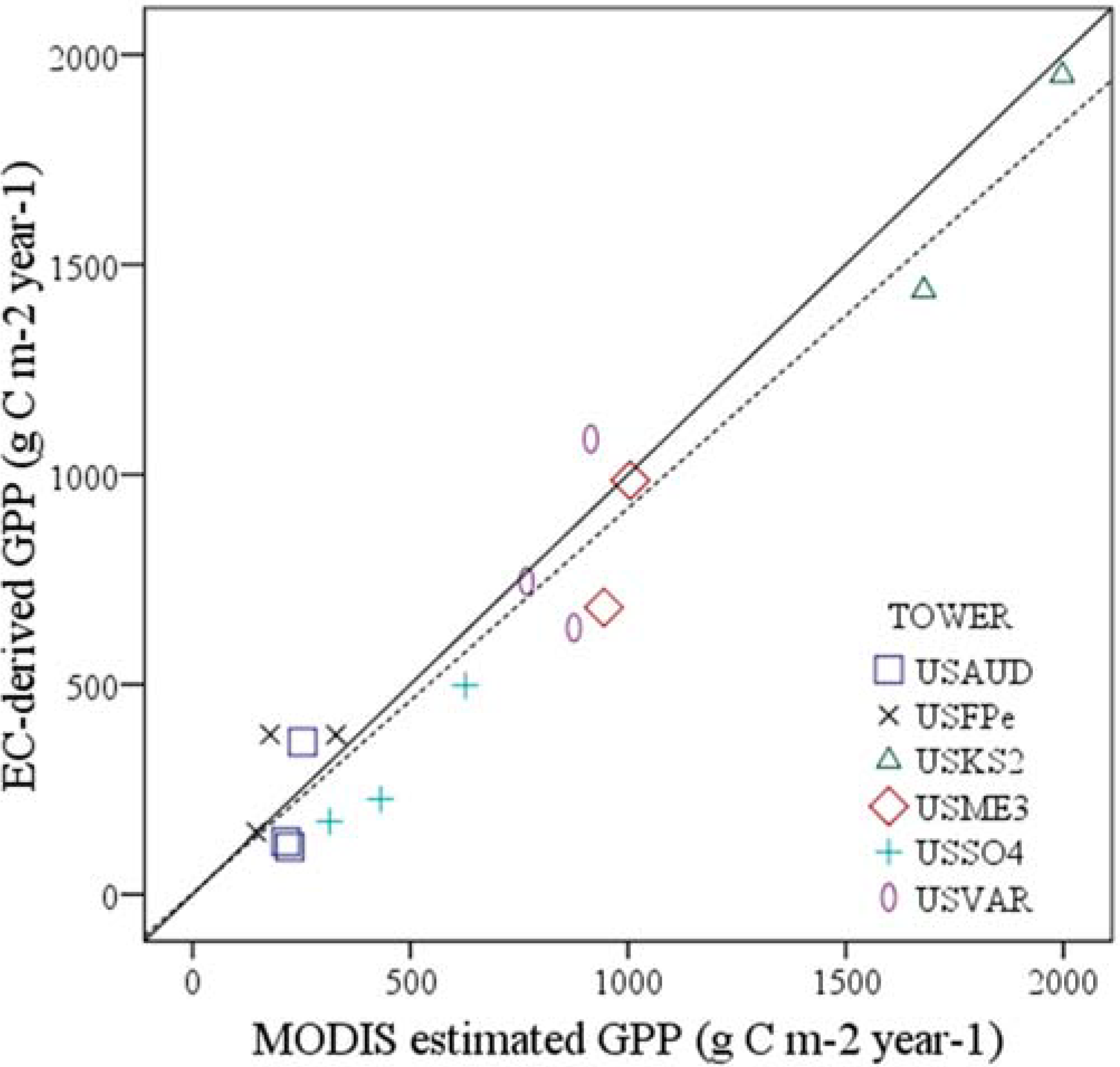
The results showed that GPPm tended to overestimate annual GPP in non-forested areas (Table 2, Figure 2). For the two sites located in shrublands (USSO4 and USKS2) water limitation might have played a role, since the overestimation was much larger for the site located in a water-limited area (USSO4) compared to non-water limited areas. This overestimation by GPPm could be attributed to the fact that the DAO meteorology used by the MOD17 algorithm underestimates local VPD in many water-limited sites during the summer, and therefore photosynthesis is not sufficiently constrained when calculating GPPm for dry periods in North America [13,42]. This result agrees with [13], who found a similar overestimation of 67% for an open shrubland site in a dry area. However, [19] found that MODIS slightly underestimated GPP in two shrublands in water deficient areas. Some authors have suggested that these limitations in dry regions can be overcome with the inclusion of the variable SWC in the MOD17 algorithm [43].
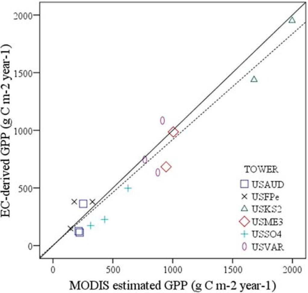
Figure 2.
Relationship between EC-derived annual GPP with MODIS annual estimated GPP. The dashed line is the linear best fit for dataset 1 (n = 12) and the solid line is the 1:1 reference.
Figure 2.
Relationship between EC-derived annual GPP with MODIS annual estimated GPP. The dashed line is the linear best fit for dataset 1 (n = 12) and the solid line is the 1:1 reference.
Since the grasslands were located in water-limited areas and taking into account the limitation of the MOD17 algorithm in underestimating water stress, we expected the annual GPP to be overestimated [13] in these sites. However, the results showed that GPP was underestimated in these three sites in 2005 (Table 2). The reason for these underestimations might be related to the fact that 2005 was categorized as “extremely moist” and “moderately moist” between April and December for the areas where those sites were located [44]. For USAUD and USVAR, the underestimation happened in both cases when there was more precipitation in comparison to the other two years. For the remaining years, GPP was overestimated in those two sites. In addition, the overestimation was larger in the site located in the dry area (Bsh) than for the site located in the temperate area (Csa). An inverse relationship was found between the magnitude of the overestimation of the GPP and the precipitation for these two sites (Table 2). The underestimation of annual GPP in USFPe in 2004 can be explained by the fact that, although there was not more annual precipitation than in the other years, most of it fell during the summer months (data not shown) and therefore the local VDP was not underestimated. These results agree with the previous explanations about the effect of VDP estimations in the MOD17 algorithm and corroborate the hypothesis that GPPm is overestimated in non-forested biomes where soil water is severely limiting during the growing season.
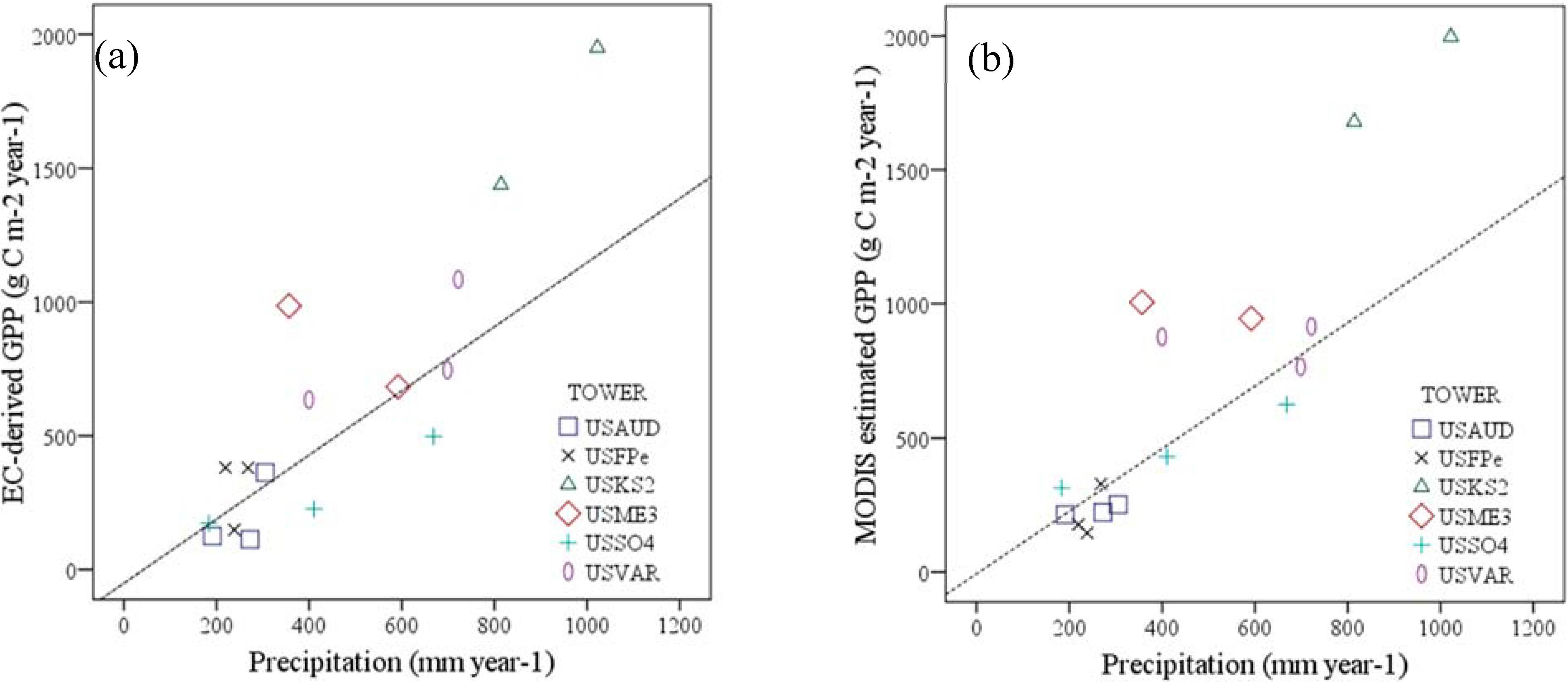
Though water content or water potential of topsoil horizons are the most desirable predictors in GPP modelling [9], such data is hard to summarise on a yearly basis and it is also not available for all the towers, making precipitation a more adequate variable to be considered. The existence of a strong correlation between annual GPP (GPPec and GPPm) and precipitation in water-limited grasslands and in shrublands (Table 3 and Figure 3a,b) agrees with the results obtained by [9]. It shows the ability of GPPec and GPPm to capture the relationship between photosynthetic activity and one limiting factor like precipitation, and it makes possible the use of this variable to improve the estimation of GPPec in non-forested biomes on an annual basis. The general predictive model which included the forested site was less accurate than the model developed for non-forested sites. Thus, we recommend the use of specific models based on data from those biomes and to use meteorological data at a finer spatial resolution than interpolated DAO data.

Table 3.
Relationship between EC-derived annual GPP (GPPec) (g C∙m−2∙year−1), MODIS annual estimated GPP (GPPm) (g C∙m−2∙year−1) and precipitation (Precip) (mm). Note: Dataset 1: grasslands and shrublands located in water limited sites (n = 12), Dataset 2: all sites located in grasslands/shrublands (n = 14), Dataset 3: all sites located in forested areas and grasslands/shrublands (n = 16), r2: coefficient of determination, SEE: Standard Error of the Estimate (g C∙m−2∙year−1). All the regressions were significant at the 95% confidence level.
| Variable Y | Variable X | Dataset | r2 | SEE |
|---|---|---|---|---|
| GPPec | GPPm | 1 | 0.77 | 149.26 |
| 2 | 0.94 | 143.36 | ||
| 3 | 0.93 | 142.57 | ||
| GPPec | Precip | 1 | 0.68 | 175.11 |
| 2 | 0.83 | 233.86 | ||
| 3 | 0.75 | 267.41 | ||
| GPPm | Precip | 1 | 0.71 | 159.51 |
| 2 | 0.83 | 249.28 | ||
| 3 | 0.77 | 272.02 |
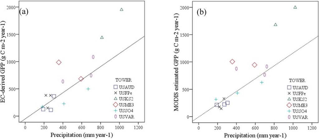
Figure 3.
Relationship between precipitation and (a) EC-derived annual GPP, (b) MODIS estimated annual GPP. The dashed line is the linear best fit for dataset 1 (n = 12).
Figure 3.
Relationship between precipitation and (a) EC-derived annual GPP, (b) MODIS estimated annual GPP. The dashed line is the linear best fit for dataset 1 (n = 12).
3.2. Suitability of the MODIS GPP Product to Estimate Temporal Dynamics of the Carbon Fluxes at Eight-Day Intervals.
The MODIS GPP algorithm is considered to be able to capture seasonal dynamics in photosynthetic production [13]. However, the eight-day interval plots showed that the temporal dynamics of C in the non-forested water-limited sites were not as well captured by MOD17 (Figure 4a–c) as for the shrubland located in a non-water deficient area (Figure 4d). The delay in capturing the end of the growing season might have been due to the incapability of the algorithm to accurately reflect the influence of low soil water content, which led to an overestimation of GPP. In all cases, the results showed that capturing the magnitude of the changes and the peak of the photosynthetic activity in the non-forested sites (regardless of the soil water availability) is still an issue, as [13] and [32] have found. Along the same lines, the largest discrepancies between GPPm and GPPec in the water-limited sites were found during periods when the photosynthetic activity was the lowest, with an overestimation for all cases except for USFPe (2005). This overestimation for sites with low productivity during the fall has been reported previously by [13]. The exception of USFPe was probably related to the unusual precipitation events which happened during those periods [44] as discussed in the previous section.
The results of the quantitative analysis of the agreement between GPPec and GPPm at eight-day intervals are showed in Table 4. All the variables in the annual dataset were normal (α = 0.05), except for the sites USAUD (all years) and USVAR (all years), where the GPPec was not normally distributed. Hence, for those sites the square of the Spearman rho coefficient of correlation (ρ) was included in the tables as a measure of agreement between GPPec and GPPm instead of the r2 (Table 4). The values estimated by Model 3 were plotted for each tower and year (Figure 4), so that they could be compared to GPPec and GPPm.
The highest agreement between GPPec and GPPm per year and tower (Model 1) was obtained for the forested site (USME3) (r2 = 0.78, SEE = 0.85, n = 45), while in the non-forested sites the agreement was lower than 65%. Analogous results were obtained for Model 2 (r2 = 0.69, SEE = 0.92, n = 89) and Model 3. Regardless of the temporal water restrictions at the forest site during the summer, the reduced seasonal variation made it easier to model the C cycle using GPPm. At the water-limited non-forested sites, the average agreement between GPPec and GPPm was lower than at the site without water restrictions. The performance of Model 1 also varied the most amongst the years in the water-limited non-forested sites. These differences between years had an impact on the accuracy of the model that took into account tower data over a number of years (Model 2), which were generally less accurate than the model that used tower data for each year separately (Model 1). None of the models for the sites located in grasslands or shrublands were able to explain more than 50% of the variance of the GPPec eight-day data using the GPPm eight-days as input.
As for the annual GPP, one reason for the discrepancies between the eight-day GPPec and GPPm might be related to the large scale of the meteorological data used by MOD17 [2,13] and the underestimation of the local VPD in the water deficient areas. The use of more accurate meteorological data (e.g., tower data) can solve this problem in some cases, but in grasslands it can lead to an underestimation of GPPm [13]. Another source of disagreement between the eight-day GPPm and GPPec is that tower based GPP represents a small, unfixed footprint that changes in size and shape as function of wind speed, wind direction, surface roughness, and atmospheric stability [32] and this variability in GPPec has a larger impact when analysing temporal dynamics than when annual GPP is considered, since for the latter these differences can be balanced over the whole year. Finally, the partitioning of the NEE into GPP and Re is another source of uncertainty which might have a larger impact on the accuracy of the seasonal dynamics than on the annual values, since it is usually modelled for a small temporal window (e.g., 10-day) [36,37], which might provide more accurate results for one part of the year and less for others. In addition, partitioning of the NEE is more complex in non-forested ecosystems located in dry areas where growth is limited by water [45].
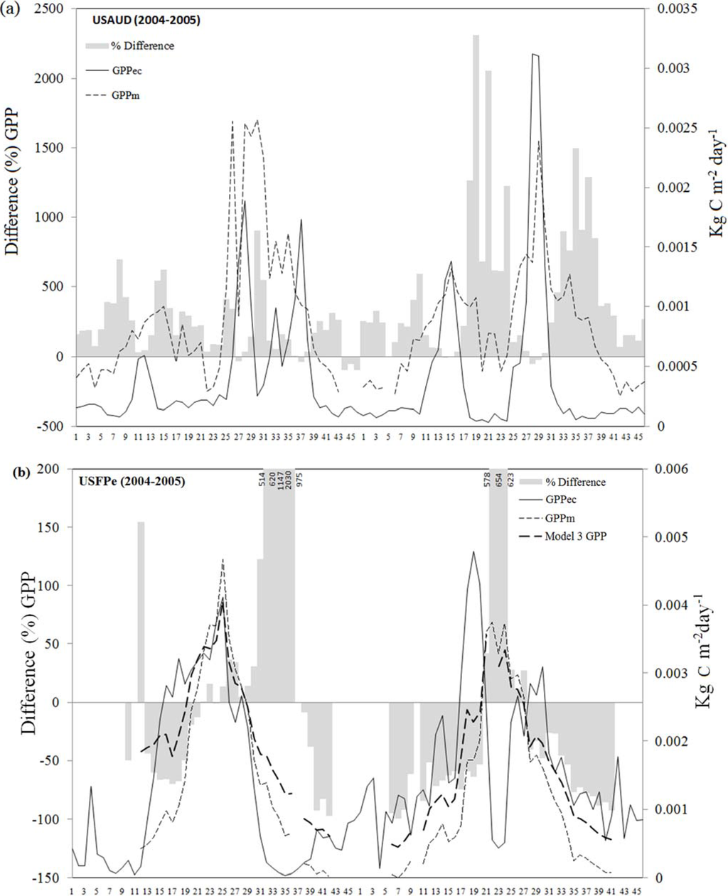
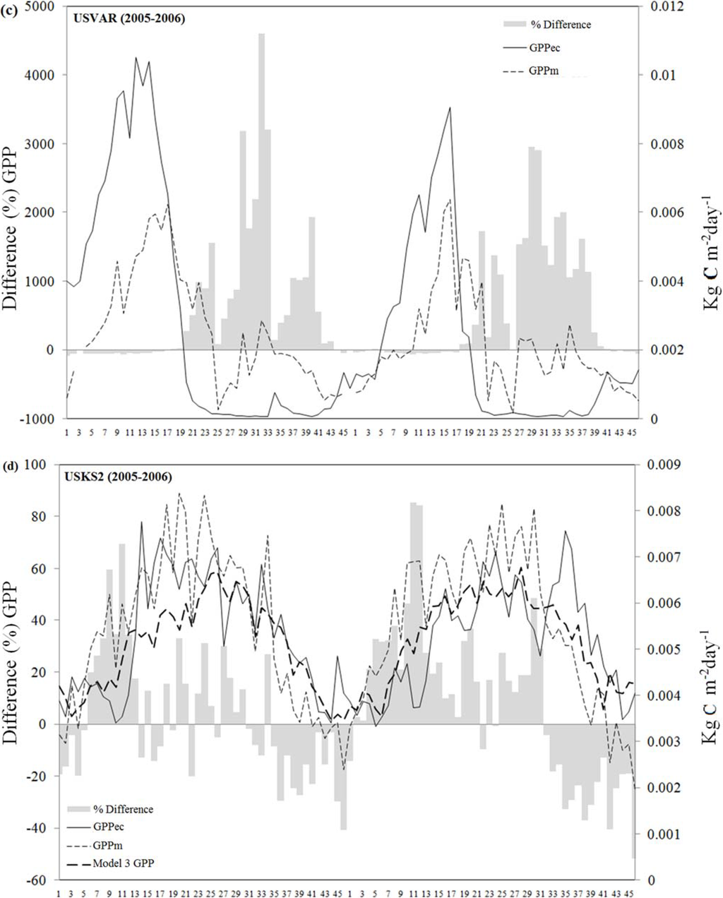
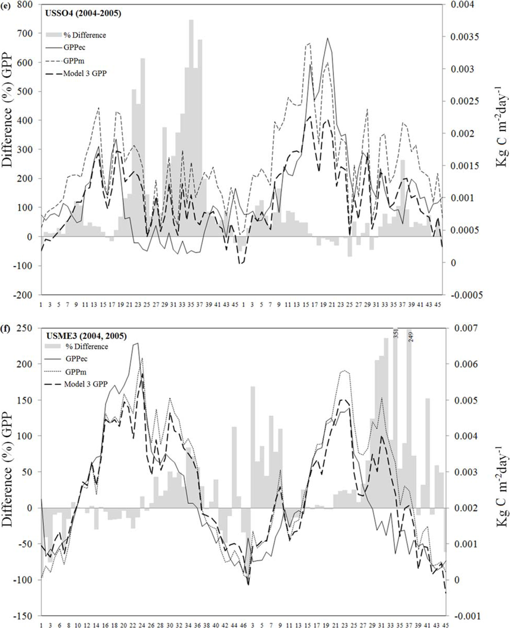
Figure 4.
Temporal trace of the eight-day observed EC-derived GPP and the percentage difference between the observed and the GPP predicted by the MODIS product (MOD17 values and estimations by Model 3 for different sites: (a) USAUD (2004–2005), (b) USFPe (2004–2005), (c) USVAR (2005–2006), (d) USKS2 (2005–2006), (e) USSO4 (2004–2005), (f) USME3 (2004, 2005). GPP measured as kg C∙m−2∙day−1. Horizontal axis represents eight-day periods. The characteristics of Model 3 for each site are shown in Table 4.
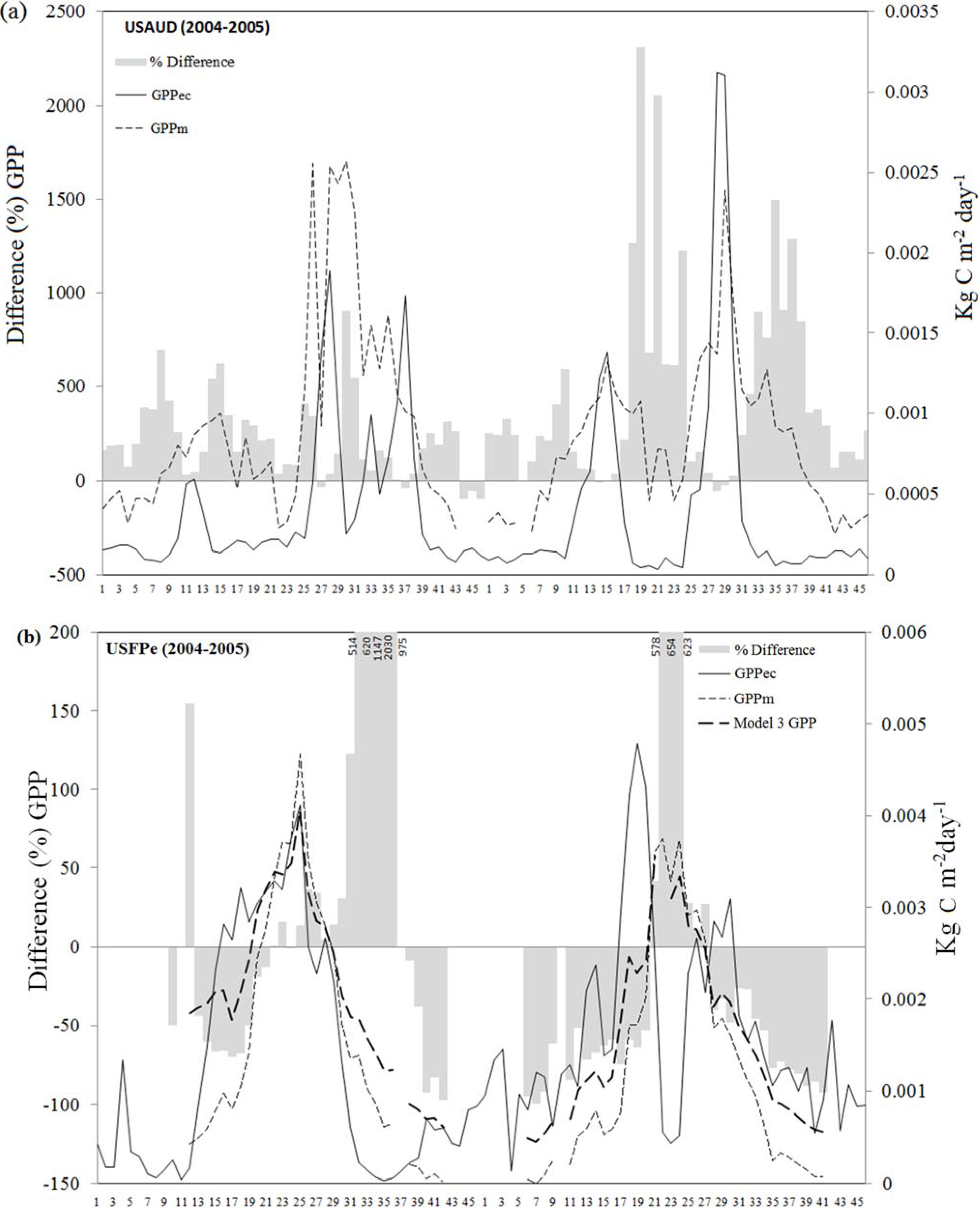


Table 4.
Relationship between MODIS estimated eight-day GPP (GPPm) with EC-derived 8-day GPP. Model 1 was adjusted per tower and per year. Model 2 was adjusted per tower. Model 3 was adjusted per tower with EC-GPP as the dependent variable and GPPm and other tower variables as independent variables. For USAUD and USVAR (not normally distributed) the Spearman rho coefficient of correlation (ρ) was calculated instead (#ρ2). Notes: coefficient of determination (r2) (in bold: r2 > 0.5, all are significant at the 95% confidence level), # indicates that ρ2 has been calculated instead of r2, standard error of the estimate (SEE) (g C∙m−2∙day−1), n: number of cases, Var: predictor variables in the model, Rg: global radiation (W∙m−2), SWC: soil water content (% volume), Ta: air temperature (ºC), Ts: soil temperature (ºC).
| Tower | Model 1 | Model 2 | Model 3 | |||||
|---|---|---|---|---|---|---|---|---|
| Year | r2/ #ρ2 | SEE | r2/ #ρ2 (n) | SEE | r2/ #ρ2 | SEE | Var | |
| USAUD | 2003 | 0.58 # | - | 0.03 # (96) | - | 0.18 # | Ts | |
| 2004 | 0.29 # | - | ||||||
| 2005 | 0.18 # | - | ||||||
| USFPe | 2004 | 0.32 | 0.73 | 0.44 (62) | 0.89 | 0.52 | 0.83 | GPPm, SWC |
| 2005 | 0.50 | 0.81 | ||||||
| 2006 | 0.57 | 0.49 | ||||||
| USVAR | 2004 | 0.02 # | - | 0.13 # (136) | - | 0.60 # | SWC | |
| 2005 | 0.37 # | - | ||||||
| 2006 | 0.14 # | - | ||||||
| USKS2 | 2005 | 0.54 | 0.89 | 0.49 | 0.88 | 0.65 | 0.75 | Ts, Rg |
| 2006 | 0.51 | 0.81 | (82) | |||||
| USSO4 | 2004 | 0.39 | 0.38 | 0.46 (104) | 0.51 | 0.50 | 0.50 | GPPm, Rg |
| 2005 | 0.46 | 0.57 | ||||||
| 2006 | 0.36 | 0.39 | ||||||
| USME3 | 2004 | 0.78 | 0.85 | 0.69 | 0.92 | 0.75 | 0.83 | GPPm, Ta |
| 2005 | 0.65 | 0.84 | (89) | |||||
3.3. Conditions/Variables Which May Affect the Suitability of the MODIS GPP Product for Estimating C Temporal Dynamics in Shrublands and Grasslands in Water Deficient Areas
The temporal dynamics of the C fluxes at eight-day intervals were improved for most sites by adding accurate information regarding soil temperature, radiation and/or water availability to the GPPm data, as Model 3 showed (Table 4, Figure 4a–f). Their inclusion in the models agrees with the fact that radiation, temperature and water have been reported by several authors as the most important factors influencing ecosystem productivity and respiration (e.g., [9,46]).
The use of global radiation and soil temperature in the model for the non-water-limited shrubland lowered the GPP overestimation for the season with very high productivity and realistically captured the onset of the season (Figure 4e). The absence of water availability in the model suggests that in this site GPP is not constrained by the amount of water available, since the critical minimum value is never reached, as found by [47] in grasslands in humid areas. The fact that soil temperature was better related to GPP than air temperature in this site agrees with the findings of [8] for a forested site, and it might have been related to a more developed radical system in comparison to a grassland area (where air temperature has a more important role [3]). For the forested site, the addition of variables related to water availability did not improve the GPP estimations, probably due to the fact that the C cycles did not have large variations (Figure 4f) due to water constraints.
The models that characterised the temporal dynamics of the GPP in grasslands and shrublands located in water-limited areas were not able to explain more than 60% of the variance of the data (see Model 3 in Table 4). Although it was not possible to find a linear relationship to model GPPec for USVAR and USAUD, since the data were not normally distributed, GPPec showed a stronger correlation with SWC than with GPPm for USVAR, highlighting the importance of water availability to obtain accurate estimations of GPP. Along the same lines, the inclusion of SWC in addition to GPPm in the model adjusted for USFPe helped correct the overestimation of GPPm during the most water-limited period, overcoming the limitations of the MOD17 algorithm due to the underestimation of VDP [13,43], and corrected the underestimation of GPPm during the beginning of the growing season, when VPD was probably overestimated. The poor performance of the model adjusted for USSO4 during the summer period of 2004 might have been due to the fact that water availability was not included as a predictor (probability of F to enter SWC in the model ≥0.05), and therefore the overestimation of GPPm could not be corrected. These results showed that soil water availability and its inclusion in the MOD17 algorithm is a critical factor in the estimation and monitoring of photosynthetic activity in non-forested water-limited sites, as reported by [13,16,32,48].
4. Conclusions
In non-forested sites in water-limited areas, the MODIS GPP product is well correlated with the GPP EC tower estimations when averaged at an annual level, although it tends to overestimate. However, the existence of occasional and large precipitation events during the growing season led to infrequent underestimations. Since there is a correlation between precipitation and GPPec in these sites, the use of precipitation data at a finer spatial resolution than DAO data can improve the accuracy in the estimations of annual GPP. However, the development of a general model based on precipitation would require a larger sample of water limited sites.
The seasonal dynamics and the beginning and end of the growing season were not well captured by GPPm in the sites where (i) the productivity was low throughout the year or (ii) the changes in the flux trend were abrupt, usually due to the restrictions in water availability. In the grasslands and shrublands located in water limited sites, water stress is the primary limiting factor that controls photosynthesis and therefore GPP; hence, soil water stress should be added to the MOD17 algorithm calculations for these dry areas. Using the existing weekly GPPm data, the GPP estimations can be improved in non-forested sites in water-limited areas by including in the model meteorological data at a finer spatial scale as well as soil water content and temperature measurements.
Acknowledgments
This work used Eddy covariance data acquired by the FLUXNET community and in particular by the following networks: AmeriFlux (US Department of Energy, Biological and Environmental Research, Terrestrial Carbon Program (DEFG0204ER63917 and DEFG0204ER63911)) and CarboEuropeIP. We acknowledge the financial support to the eddy covariance data harmonization provided by CarboEuropeIP and US Department of Energy and the database development and technical support from Berkeley Water Center, Lawrence Berkeley National Laboratory, Microsoft Research eScience, Oak Ridge National Laboratory, University of California Berkeley, University of Virginia.
This research was developed during an internship at the Natural Resources Department, ITC (University of Twente), Enschede, Netherlands, funded by the Leonardo da Vinci/Erasmus Programme.
This research was developed during an internship at the Natural Resources Department, ITC (University of Twente), Enschede, Netherlands, funded by the Programme for Young Researchers “José Castillejo” (Spanish Ministry of Education) (JC2010-0132).
Author Contributions
The authors contributed equally to this work. Flor Álvarez-Taboada and David Tammadge carried out the data preprocessing, modelling and validation, and wrote some sections of the paper. Martin Schlerf and Andrew Skidmore supervised the data preprocessing, modelling and validation, and wrote some sections of the paper.
Conflicts of Interest
The authors declare no conflict of interest.
References
- Jarvis, P.G. Global change and terrestrial ecosystems in monsoon Asia. Vegetation 1995, 121, 157–174. [Google Scholar] [CrossRef]
- Coops, N.C.; Black, T.A.; Jassal, R.S.; Trofymow, J.A.; Morgenstern, K. Comparison of MODIS, eddy covariance determined and physiologically modelled gross primary production (GPP) in a Douglas-fir forest stand. Remote Sens. Environ. 2007, 107, 385–401. [Google Scholar] [CrossRef]
- Goulden, M.L.; Daube, B.C.; Fan, S.M.; Sutton, D.J.; Bazzaz, A.; Munger, J.W.; Wofsy, S.C. Physiological responses of a black spruce forest to weather. J. Geophys. Res. Atmos. 1997, 102, 28987–28996. [Google Scholar] [CrossRef]
- Huang, H.; Zhang, J.; Meng, P.; Fu, Y.; Zheng, N.; Gao, J. Seasonal variation and meteorological control of CO2 flux in a hilly plantation in the mountain areas of North China. Acta Meteorol. Sinica 2011, 25, 238–248. [Google Scholar] [CrossRef]
- Morgenstern, K.; Black, T.A.; Humphrey, E.R.; Griffis, T.J.; Drewitt, G.B.; Cai, T.; Nesic, Z.; Livingston, N.J. Sensitivity and uncertainty of the carbon balance of a Pacific Northwest Douglas-fir forest during an El Niño/La Niña cycle. Agr. Forest Meteorol. 2004, 123, 201–219. [Google Scholar] [CrossRef]
- Thomas, M.V.; Malhi, Y.; Fenn, K.M.; Fisher, J.B.; Morecroft, M.D.; Lloyd, C.R.; Taylor, M.E.; McNeil, D.D. Carbon dioxide fluxes over an ancient broadleaved deciduous woodland in southern England. Biogeosciences 2011, 8, 1595–1613. [Google Scholar] [CrossRef]
- Valentini, R.; Matteucci, G.; Dolman, A.J.; Schulze, E.D.; Rebmann, C.; Moors, E.J.; Granier, A.; Gross, P.; Jensen, N.O.; Pilegaard, K.; et al. Respiration as the main determinant of carbon balance in European forests. Nature 2000, 404, 861–865. [Google Scholar] [CrossRef] [PubMed]
- Van Dijk, A.I.J.M.; Dolman, A.J. Estimates of CO2 uptake and release among European forests based on eddy covariance data. Glob. Change Biol. 2004, 10, 1445–1459. [Google Scholar] [CrossRef]
- Gilmanov, T.G.; Aires, L.; Belelli, L.; Barcza, Z.; Baron, V.S.; Beringer, J.; Billesbach, D.; Bonal, D.; Bradford, J.; Ceschia, E.; et al. Productivity, respiration, and light-response parameters of world grassland and agroecosystems derived from flux-tower measurements. Rangeland Ecol. Manag. 2010, 63, 16–39. [Google Scholar] [CrossRef]
- Gebremichael, M.; Barros, A.P. Evaluation of MODIS gross primary productivity (GPP) in tropical monsoon regions. Remote Sens. Environ. 2006, 100, 150–166. [Google Scholar] [CrossRef]
- Wu, C.; Chen, J.M. The use of precipitation intensity in estimating gross primary production in four northern grasslands. J. Arid Environ. 2012, 82, 11–18. [Google Scholar] [CrossRef]
- Ham, J.M.; Knapp, A.K. Fluxes of CO2, water vapor, and energy from a prairie ecosystem during the seasonal transition from carbon sink to carbon source. Agr. Forest Meteorol. 1998, 89, 1–14. [Google Scholar] [CrossRef]
- Heinsch, F.A.; Zhao, M.; Running, S.W.; Kimball, J.S.; Nemani, R.R.; Davis, K.J.; Bolstad, P.V.; Cook, B.D.; Desai, A.R.; Ricciuto, D.M.; et al. Evaluation of remote sensing based terrestrial productivity from MODIS using regional tower eddy flux network observations. IEEE Trans. Geosci. Remote Sens. 2006, 44, 1908–1925. [Google Scholar] [CrossRef]
- Goulden, M.L.; Munger, W.; Fan, S.; Daube, B.C.; Wofsy, S.C. Measurements of carbon sequestration by long-term eddy covariance: Methods and a critical evaluation of accuracy. Glob. Change Biol. 1996, 2, 169–182. [Google Scholar] [CrossRef]
- Desai, A.R.; Richardson, A.D.; Moffa, A.M.; Kattge, J.; Hollinger, D.Y.; Barr, A.; Falge, E.; Noormets, A.; Papale, D.; Reichstein, M.; et al. Cross-site evaluation of eddy covariance GPP and RE decomposition techniques. Agr. Forest Meteorol. 2008, 148, 821–838. [Google Scholar] [CrossRef]
- Turner, D.P.; Urbanski, S.; Wofsy, S.C.; Bremer, D.J.; Gower, S.T.; Gregory, M. A cross-biome comparison of light use efficiency for gross primary production. Glob. Change Biol. 2003, 9, 383–395. [Google Scholar] [CrossRef]
- Baldocchi, D.; Falge, E.; Gu, L.; Olson, R.; Hollinger, D.; Running, S.; Anthoni, P.; Bernhofer, C.; Davis, K.; Evans, R.; et al. FLUXNET: A new tool to study the temporal and spatial variability of ecosystem-scale carbon dioxide, water vapor, and energy flux densities. Bull. Am. Meteorol. Soc. 2001, 82, 2415–2434. [Google Scholar] [CrossRef]
- Xiao, J.; Zhuang, Q.; Law, B.E.; Chen, J.; Baldocchi, D.D.; Cook, D.R.; Oren, D.; Richardson, A.D.; Wharton, S.; Ma, S.; et al. A continuous measure of gross primary production for the conterminous United States derived from MODIS and AmeriFlux data. Remote Sens. Environ. 2010, 114, 576–591. [Google Scholar] [CrossRef]
- Coops, N.C.; Waring, R.H. The use of multi-scale remote sensing imagery to derive regional estimates of forest growth capacity using 3-PGS. Remote Sens. Environ. 2001, 75, 324–334. [Google Scholar] [CrossRef]
- Landsberg, J.J.; Waring, R.H. A generalized model of forest productivity using simplified concepts of radiation-use efficiency, carbon balance, and partitioning. Forest Ecol. Manag. 1997, 95, 209–228. [Google Scholar] [CrossRef]
- Li, Z.Q.; Yu, G.R.; Xiao, X.M.; Li, Y.N.; Zha, X.Q.; Ren, C.Y.; Zhang, L.M.; Fu, Y.L. Modelling gross primary production of alpine ecosystems in the Tibetan Plateau using MODIS images and climate data. Remote Sens. Environ. 2007, 107, 510–519. [Google Scholar] [CrossRef]
- Turner, D.P.; Ritts, W.D.; Cohen, W.B.; Gower, S.T.; Running, S.W.; Zhao, M.; Costa, M.H.; Kirschbaum, A.A.; Ham, J.; Saleska, S.; et al. Evaluation of MODIS NPP and GPP products across multiple biomes. Remote Sens. Environ. 2006, 102, 282–292. [Google Scholar] [CrossRef]
- Drolet, G.G.; Middleto, E.M.; Huemmrich, K.F.; Hall, F.G.; Amiro, B.D.; Barr, A.G.; Black, T.A.; McCaughey, J.H.; Margolis, H.A. Regional mapping of gross light-use efficiency using MODIS spectral indices. Remote Sens. Environ. 2008, 112, 3064–3078. [Google Scholar] [CrossRef]
- Veroustraete, F.; Patyn, J.; Myneni, R.B. Estimating net ecosystem exchange of carbon using the normalized difference vegetation index and an ecosystem model. Remote Sens. Environ. 1996, 58, 115–130. [Google Scholar] [CrossRef]
- Xiao, X.; Hollinger, D.; Aber, J.D.; Goltz, M.; Davidson, E.A.; Zhang, Q.Y. Satellite-based modeling of gross primary production in an evergreen needleleaf forest. Remote Sens. Environ. 2004, 89, 519–534. [Google Scholar] [CrossRef]
- Xiao, X.; Zhang, Q.; Braswell, B.; Urbanski, S.; Boles, S.; Wofsy, S.C.; Moore III, B.; Ojima, D. Modeling gross primary production of a deciduous broadleaf forest using satellite images and climate data. Remote Sens. Environ. 2004, 91, 256–270. [Google Scholar] [CrossRef]
- Running, S.W.; Nemani, R.R.; Heinsch, F.A.; Zhao, M.; Reeves, M.; Jolly, M. A continuous satellite-derived measure of global terrestrial primary productivity: Future science and applications. Bioscience 2004, 56, 547–560. [Google Scholar] [CrossRef]
- Data Assimilation Office (DAO); (Goddard Space Flight Center, Greenbelt, MD, USA). Algorithm Theoretical Basis Document (ATBD). Unpublished word. 2002. [Google Scholar]
- Turner, D.P.; Ritts, W.D.; Zhao, M.; Kurc, S.A.; Dunn, A.L.; Wofsy, S.C.; Small, E.E.; Running, S.W. Assessing interannual variation in MODIS-based estimates of gross primary production. IEEE Trans. Geosci. Remote Sens. 2006, 44, 1899–1907. [Google Scholar] [CrossRef]
- Goerner, A.; Reichstein, M.; Rambal, S. Tracking seasonal drought effects on ecosystem light use efficiency with satellite-based PRI in a Mediterranean forest. Remote Sens. Environ. 2009, 113, 1101–1111. [Google Scholar] [CrossRef]
- Chasmer, L.; Barr, A.; Hopkinson, C.; McCaughey, H.; Treitz, P.; Black, A. Scaling and assessment of GPP from MODIS using a combination of airborne LiDAR and eddy covariance measurements over jack pine forests. Remote Sens. Environ. 2009, 113, 82–93. [Google Scholar] [CrossRef]
- Zhang, L.; Wylie, B.; Loveland, T.; Fosnight, E.; Tieszen, L.L.; Ji, L.; Gilmanov, T. Evaluation and comparison of gross primary production estimates for the Northern Great Plains grasslands. Remote Sens. Environ. 2007, 106, 173–189. [Google Scholar] [CrossRef]
- Köppen, W.; Geiger, R. Das geographische system der klimate. In Handbuch der Klimatologie; Verlag Gebrüder Bornträger: Berlin, Germany, 1936. [Google Scholar]
- Ameriflux Website. Available online: http://public.ornl.gov/ameriflux/ (accessed on 28 November 2014).
- Moffat, A.M.; Papale, D.; Reichstein, M.; Hollinger, D.Y.; Richardson, A.D.; Barr, A.G.; Beckstein, C.; Braswell, B.H.; Churkina, G.; Desai, A.R.; et al. Comprehensive comparison of gap filling techniques for eddy covariance net carbon fluxes. Agr. Forest Meteorol. 2007, 147, 209–232. [Google Scholar] [CrossRef]
- Lasslop, G.; Reichstein, M.; Papale, D.; Richardson, A.D.; Arneth, A.; Barr, A.; Stoy, P.; Wohlfahrt, G. Separation of net ecosystem exchange into assimilation and respiration using a light response curve approach: Critical issues and global evaluation. Glob. Change Biol. 2010, 16, 187–208. [Google Scholar] [CrossRef]
- Reichstein, M.; Falge, E.; Baldocchi, D.; Aubinet, M.; Berbigier, P.; Bernhofer, C.; Buchmann, N.; Falk, M.; Gilmanov, T.; Granier, A.; et al. On the separation of net ecosystem exchange into assimilation and ecosystem respiration: Review and improved algorithm. Glob. Change Biol. 2005, 11, 1424–1439. [Google Scholar] [CrossRef]
- Wolf, S.; Eugste, W.; Potvin, C.; Turner, B.; Buchmann, N. Carbon sequestration potential of tropical pasture compared with afforestation in Panama. Glob. Change Biol. 2011, 17, 2763–2780. [Google Scholar] [CrossRef]
- Oak Ridge National Laboratory Distributed Active Archive Center. MODIS Subsetted Land Products, Collection 5. Available online: http://daac.ornl.gov/MODIS/modis.html (accessed on 28 November 2014).
- Running, S.; Zhao, M. Note on Use of MODIS GPP/NPP (MOD17) Data Set. Available online: ftp://daac.ornl.gov/data/modis_ascii_subsets/C5_MOD17A2/mod17_NTSG.pdf (accessed on 28 November 2014).
- Corder, G.W.; Foreman, D.I. Nonparametric Statistics for Non-Statisticians: A Step-by-Step Approach; Wiley: Hoboken, NJ, USA, 2009. [Google Scholar]
- Zhao, L.; Gu, S.; Yu, G.; Zhao, X.; Li, Y.; Xu, S.; Zhou, H. Diurnal, seasonal and annual variation in net ecosystem CO2 exchange of an alpine shrubland on Qinghai-Tibetan plateau. Glob. Change Biol. 2006, 12, 1940–1953. [Google Scholar] [CrossRef]
- Mu, Q.M.; Heinsch, F.A.; Liu, M.; Tian, H.; Running, S.W. Evaluating water stress controls on primary production in biogeological and remote sensing based models. J. Geophys. Res. 2007, 112. [Google Scholar] [CrossRef]
- NOAA. Drought—Annual 2005. Available online: http://www.ncdc.noaa.gov/sotc/drought/2005/13 (accessed on 28 November 2014).
- Serrano-Ortiz, P. Intercambios De CO2 Entre Atmósfera y Ecosistemas Kársticos: Aplicabilidad De Las Técnicas Comúnmente Empleadas; Universidad de Granada: Granada, Spain, 2008. [Google Scholar]
- Slatyer, R.O. Plant-Water Relationships; Academic Press: New York, NY, USA, 1967. [Google Scholar]
- Jaksic, V.; Kiely, G.; Albertson, J.; Oren, R.; Katul, G.; Leahy, P.; Byrne, K.A. Net ecosystem exchange of grassland in contrasting wet and dry years. Agr. Forest Meteorol. 2006, 139, 323–334. [Google Scholar] [CrossRef]
- Perez-Quezada, J.F.; Bown, H.E.; Fuentes, J.P.; Alfaro, F.A.; Franck, N. Effects of afforestation on soil respiration in an arid shrubland in Chile. J. Arid Environ. 2012, 83, 45–53. [Google Scholar] [CrossRef]
© 2015 by the authors; licensee MDPI, Basel, Switzerland. This article is an open access article distributed under the terms and conditions of the Creative Commons Attribution license (http://creativecommons.org/licenses/by/4.0/).
