
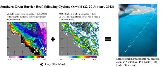
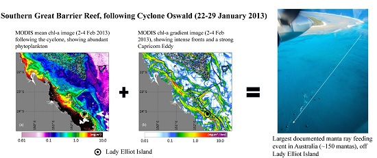
Unique Sequence of Events Triggers Manta Ray Feeding Frenzy in the Southern Great Barrier Reef, Australia

 ,
,
Abstract
:
1. Introduction
2. Data and Methods
2.1. Manta Ray Sightings

2.2. Weather Conditions
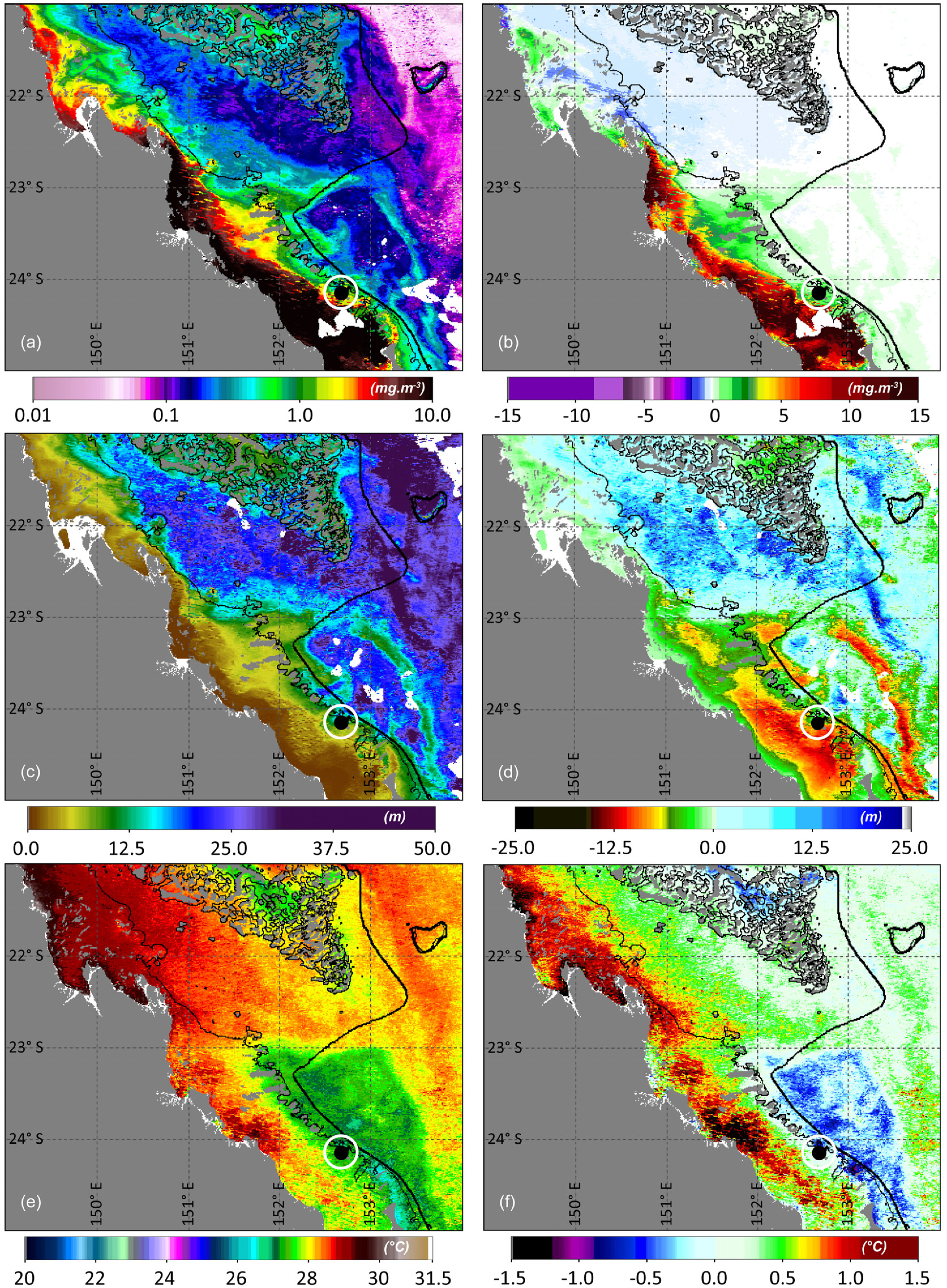
2.3. Satellite Data
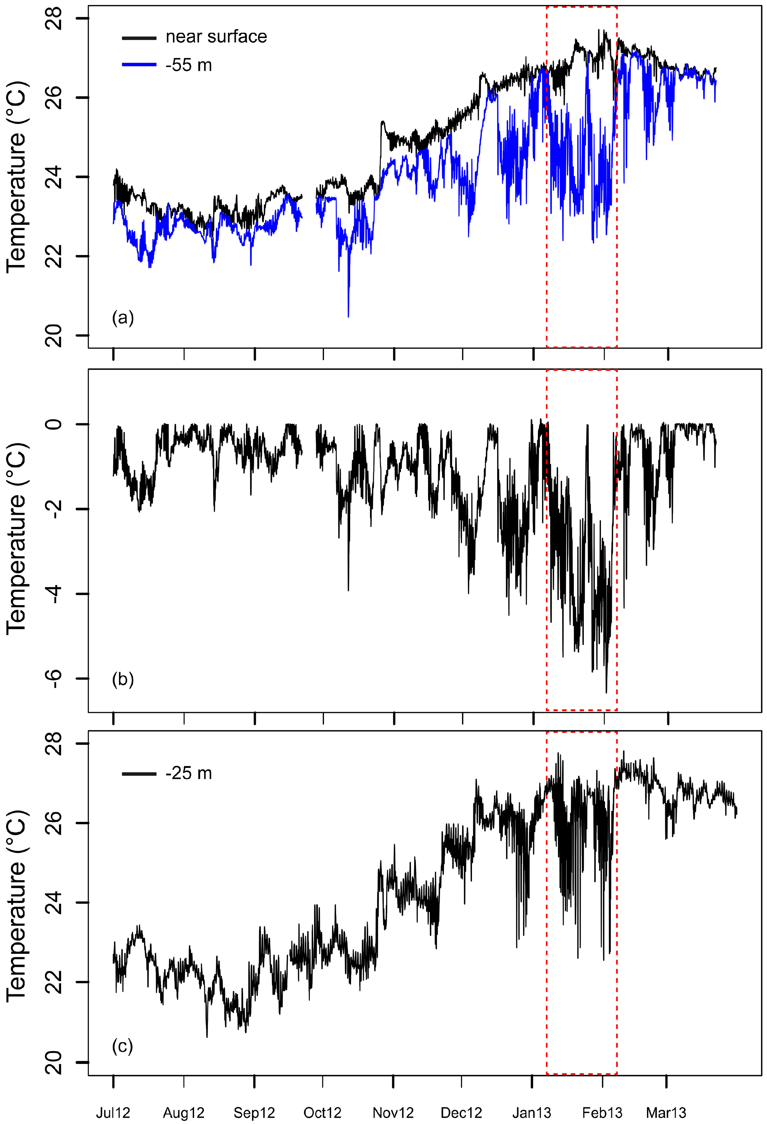
2.4. In Situ Data
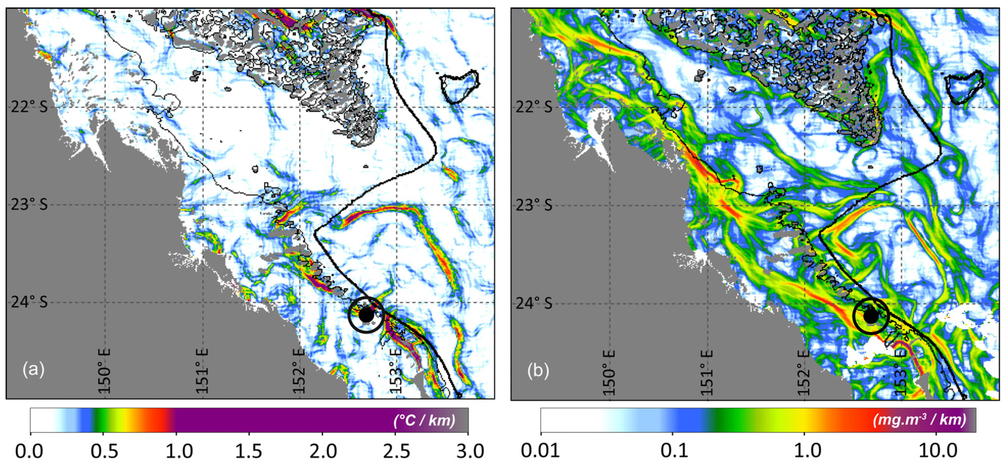
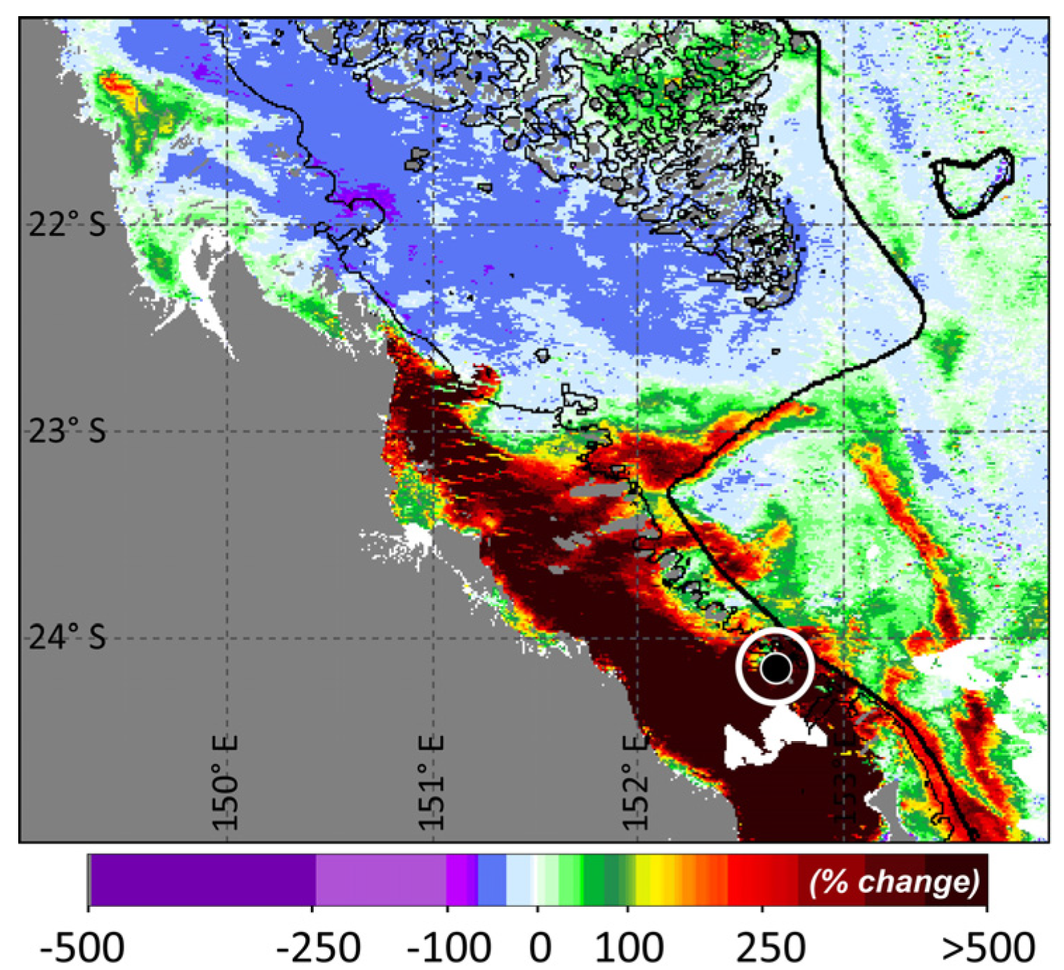
3. Results and Discussion


Ocean Fronts

4. Concluding Remarks
Acknowledgments
Author Contributions
Appendix

Conflicts of Interest
References
- Couturier, L.I.E.; Jaine, F.R.A.; Townsend, K.A.; Weeks, S.J.; Richardson, A.J.; Bennett, M.B. Distribution, site affinity and regional movements of the Manta Ray, Manta Alfredi (krefft, 1868), along the east coast of Australia. Mar. Freshw. Res. 2011, 62, 628–637. [Google Scholar] [CrossRef]
- Jaine, F.R.A.; Rohner, C.A.; Weeks, S.J.; Couturier, L.I.E.; Bennett, M.B.; Townsend, K.A.; Richardson, A.J. Movements and habitat use of reef manta rays off eastern Australia: Offshore excursions, deep diving and eddy affinity revealed by satellite telemetry. Mar. Ecol. Prog. Ser. 2014, 510, 73–86. [Google Scholar] [CrossRef]
- Couturier, L.I.E.; Dudgeon, C.L.; Pollock, K.H.; Jaine, F.R.A.; Bennett, M.B.; Townsend, K.A.; Weeks, S.J.; Richardson, A.J. Population dynamics of the reef manta ray Manta alfredi in eastern Australia. Coral Reefs 2014, 33, 329–342. [Google Scholar] [CrossRef]
- Jaine, F.R.A.; Couturier, L.I.E.; Weeks, S.J.; Townsend, K.A.; Bennett, M.B.; Fiora, K.; Richardson, A.J. When giants turn up: Sighting trends, environmental influences and habitat use of the manta ray Manta alfredi at a coral reef. PLoS One 2012, 7, e46170. [Google Scholar] [CrossRef] [PubMed]
- Weeks, S.; Bakun, A.; Steinberg, C.; Brinkman, R.; Hoegh-Guldberg, O. The Capricorn Eddy: A prominent driver of the ecology and future of the southern Great Barrier Reef. Coral Reefs 2010, 29, 975–985. [Google Scholar] [CrossRef]
- Couturier, L.I.E.; Rohner, C.A.; Richardson, A.J.; Marshall, A.D.; Jaine, F.R.A.; Bennett, M.B.; Townsend, K.A.; Weeks, S.J.; Nichols, P.D. Stable isotope and signature fatty acid analyses suggest reef manta rays feed on demersal zooplankton. PLoS One 2013, 8, e77152. [Google Scholar] [CrossRef] [PubMed]
- Richardson, A.J. In hot water: Zooplankton and climate change. ICES J. Mar. Sci. 2008, 65, 279–295. [Google Scholar] [CrossRef]
- Andrews, J.C.; Gentien, P. Upwelling as a source of nutrients for the great barrier reef ecosystems: A solution to darwin’s question? Mar. Ecol. Prog. Ser. 1982, 8, 257–269. [Google Scholar] [CrossRef]
- Bakun, A. Patterns in the Ocean: Ocean Processes and Marine Population Dynamics; University of California Sea Grant: San Diego, CA, USA, 1996; p. 323. [Google Scholar]
- Dagg, M.; Benner, R.; Lohrenz, S.; Lawrence, D. Transformation of dissolved and particulate materials on continental shelves influenced by large rivers: Plume processes. Cont. Shelf Res. 2004, 24, 833–858. [Google Scholar] [CrossRef]
- Brodie, J.; Schroeder, T.; Rohde, K.; Faithful, J.; Masters, B.; Dekker, A.; Brando, V.; Maughan, M. Dispersal of suspended sediments and nutrients in the Great Barrier Reef lagoon during river-discharge events: Conclusions from satellite remote sensing and concurrent flood-plume sampling. Mar. Freshw. Res. 2010, 61, 651–664. [Google Scholar] [CrossRef]
- McKinnon, A.D.; Thorrold, S.R. Zooplankton community structure and copepod egg production in coastal waters of the central Great Barrier Reef lagoon. J. Plankton Res. 1993, 15, 1387–1411. [Google Scholar] [CrossRef]
- Thorrold, S.R.; McKinnon, A.D. Responses of larval assemblages to a riverine plume in coastal waters of the central Great Barrier Reef. Limnol. Oceanogr. 1995, 40, 177–181. [Google Scholar] [CrossRef]
- Devlin, M.J.; Brodie, J. Terrestrial discharge into the Great Barrier Reef lagoon: Nutrient behavior in coastal waters. Mar. Pollut. Bull. 2005, 51, 9–22. [Google Scholar] [CrossRef] [PubMed]
- Kleypas, J.A.; Burrage, D.M. Satellite observations of circulation in the southern Great Barrier Reef, Australia. Int. J. Remote Sens. 1994, 15, 2051–2063. [Google Scholar] [CrossRef]
- Brown, O.B.; Minnett, P.J. MODIS Infrared Sea Surface Temperature Algorithm, Algorithm Theoretical Basis Document, v2.0; University of Miami: Miami, FL, USA, 1999. [Google Scholar]
- O’Reilly, J.E.; Coauthors, A. Seawifs Postlaunch Calibration and Validation Analyses, Part 3; NASA Goddard Space Flight Center, NASA: Washington, DC, USA, 2000; p. 49.
- Weeks, S.; Werdell, P.J.; Schaffelke, B.; Canto, M.; Lee, Z.; Wilding, J.G.; Feldman, G.C. Satellite-derived photic depth on the Great Barrier Reef: Spatio-temporal patterns of water clarity. Remote Sens. 2012, 4, 3781–3795. [Google Scholar] [CrossRef]
- Lee, Z.; Carder, K.L.; Arnone, R.A. Deriving inherent optical properties from water color: A multiband quasi-analytical algorithm for optically deep waters. Appl. Opt. 2002, 41, 5755–5772. [Google Scholar] [CrossRef] [PubMed]
- Lee, Z.P.; Weidemann, A.; Kindle, J.; Arnone, R.; Carder, K.L.; Davis, C. Euphotic zone depth: Its derivation and implication to ocean-color remote sensing. Geophys. Res. 2007, 112, 1–11. [Google Scholar]
- Mühlenstädt, T.; Kuhnt, S. Kernel interpolation. Comput. Stat. Data Anal. 2011, 55, 2962–2974. [Google Scholar] [CrossRef]
- Thompson, R.O.R.Y. Low-pass filters to suppress inertial and tidal frequencies. J. Phys. Oceanogr. 1983, 13, 1077–1083. [Google Scholar] [CrossRef]
- Da Silva, E.T.; Devlin, M.; Wenger, A.; Petus, C. Burnett-Mary Wet Season 2012–2013: Water Quality Data Sampling, Analysis and Comparison against Wet Season 2010–2011 Data; James Cook University: Townsville, QLD, Australia, 2013; p. 31. [Google Scholar]
- Waterhouse, J.; Brodie, J.; Lewis, S.; Mitchell, A. Quantifying the sources of pollutants in the Great Barrier Reef catchments and the relative risk to reef ecosystems. Mar. Pollut. Bull. 2012, 65, 394–406. [Google Scholar] [CrossRef] [PubMed]
- Kroon, F.J.; Kuhnert, P.M.; Henderson, B.L.; Wilkinson, S.N.; Kinsey-Henderson, A.; Abbott, B.; Brodie, J.E.; Turner, R.D.R. River loads of suspended solids, nitrogen, phosphorus and herbicides delivered to the Great Barrier Reef lagoon. Mar. Pollut. Bull. 2012, 65, 167–181. [Google Scholar] [CrossRef] [PubMed]
- Fabricius, K.E.; Logan, M.; Weeks, S.; Brodie, J. The effects of river run-off on water clarity across the central Great Barrier Reef. Mar. Pollut. Bull. 2014, 84, 191–200. [Google Scholar] [CrossRef] [PubMed]
- Alvarez-Romero, J.G.; Devlin, M.; Da Silva, E.T.; Petus, C.; Ban, N.C.; Pressey, R.L.; Kool, J.; Roberts, J.J.; Cerdeira-Estrada, S.; Wenger, A.S.; et al. A novel approach to model exposure of coastal-marine ecosystems to riverine flood plumes based on remote sensing techniques. J. Environ. Manag. 2013, 119, 194–207. [Google Scholar] [CrossRef]
- Bakun, A. Fronts and eddies as key structures in the habitat of marine fish larvae: Opportunity, adaptive response and competitive advantage. Sci. Mar. 2006, 70, 105–122. [Google Scholar] [CrossRef]
- Scales, K.L.; Miller, P.I.; Hawkes, L.A.; Ingram, S.N.; Sims, D.W.; Votier, S.C. On the front line: Frontal zones as priority at-sea conservation areas for mobile marine vertebrates. J. Appl. Ecol. 2014, 51, 1575–1583. [Google Scholar] [CrossRef]
- Bertrand, A.; Gerlotto, F.; Bertrand, S.; Gutierrez, M.; Alza, L.; Chipollini, A.; Diaz, E.; Espinoza, P.; Ledesma, J.; Quesquen, R.; et al. Schooling behaviour and environmental forcing in relation to anchoveta distribution: An analysis across multiple spatial scales. Prog. Oceanogr. 2008, 79, 264–277. [Google Scholar] [CrossRef]
- Sabarros, P.; Ménard, F.; Lévénez, J.; Tew-Kai, E.; Ternon, J. Mesoscale eddies influence distribution and aggregation patterns of micronekton in the Mozambique Channel. Mar. Ecol. Prog. Ser. 2009, 395, 101–107. [Google Scholar] [CrossRef]
- Godo, O.R.; Samuelsen, A.; Macaulay, G.J.; Patel, R.; Hjollo, S.S.; Horne, J.; Kaartvedt, S.; Johannessen, J.A. Mesoscale eddies are oases for higher trophic marine life. PLoS One 2012, 7, 1–9. [Google Scholar] [CrossRef]
- Richardson, A.J.; Verheye, H.M. The relative importance of food and temperature to copepod egg production and somatic growth in the southern Benguela upwelling system. J. Plankton Res. 1998, 20, 2379–2399. [Google Scholar] [CrossRef]
- Brodie, J.E.; Kroon, F.J.; Schaffelke, B.; Wolanski, E.C.; Lewis, S.E.; Devlin, M.J.; Bohnet, I.C.; Bainbridge, Z.T.; Waterhouse, J.; Davis, A.M. Terrestrial pollutant runoff to the Great Barrier Reef: An update of issues, priorities and management responses. Mar. Pollut. Bull. 2012, 65, 81–100. [Google Scholar] [CrossRef] [PubMed]
- Estrade, P.; Middleton, J.H. A numerical study of island wake generated by an elliptical tidal flow. Cont. Shelf Res. 2010, 30, 1120–1135. [Google Scholar] [CrossRef]
- O’Shea, O.R.; Kingsford, M.J.; Seymour, J. Tide-related periodicity of manta rays and sharks to cleaning stations on a coral reef. Mar. Freshw. Res. 2010, 61, 65–73. [Google Scholar] [CrossRef]
- Andrade, I.; Sangrà, P.; Hormazabal, S.; Correa-Ramirez, M. Island mass effect in the Juan Fernández archipelago (33° S), Southeastern Pacific. Deep Sea Res. I Oceanogr. Res. Pap. 2014, 84, 86–99. [Google Scholar] [CrossRef]
- Armstrong, A. Where can I Find a Decent Meal? Foraging Conditions at an Aggregation Site for Reef Manta Rays on the Great Barrier Reef; University of Queensland: Brisbane, Australia, 2014. [Google Scholar]
- Marshall, A.D.; Bennett, M.B. The frequency and effect of shark-inflicted bite injuries to the reef manta ray Manta alfredi. Afr. J. Mar. Sci. 2010, 32, 573–580. [Google Scholar] [CrossRef]
- Miller, P.I.; Christodoulou, S. Frequent locations of oceanic fronts as an indicator of pelagic diversity: Application to marine protected areas and renewables. Mar. Policy 2013, 45, 318–329. [Google Scholar] [CrossRef]
- Polovina, J.J.; Howell, E.; Kobayashi, D.R.; Seki, M.P. The transition zone chlorophyll front, a dynamic global feature defining migration and forage habitat for marine resources. Prog. Oceanogr. 2001, 49, 469–483. [Google Scholar] [CrossRef]
- Bost, C.A.; CottÈ, C.; Bailleul, F.; Cherel, Y.; Charrassin, J.B.; Guinet, C.; Ainley, D.G.; Weimerskirch, H. The importance of oceanographic fronts to marine birds and mammals of the Southern Oceans. J. Mar. Syst. 2009, 78, 363–376. [Google Scholar] [CrossRef]
© 2015 by the authors; licensee MDPI, Basel, Switzerland. This article is an open access article distributed under the terms and conditions of the Creative Commons Attribution license (http://creativecommons.org/licenses/by/4.0/).
Share and Cite
Weeks, S.J.; Magno-Canto, M.M.; Jaine, F.R.A.; Brodie, J.; Richardson, A.J. Unique Sequence of Events Triggers Manta Ray Feeding Frenzy in the Southern Great Barrier Reef, Australia. Remote Sens. 2015, 7, 3138-3152. https://doi.org/10.3390/rs70303138
Weeks SJ, Magno-Canto MM, Jaine FRA, Brodie J, Richardson AJ. Unique Sequence of Events Triggers Manta Ray Feeding Frenzy in the Southern Great Barrier Reef, Australia. Remote Sensing. 2015; 7(3):3138-3152. https://doi.org/10.3390/rs70303138
Chicago/Turabian StyleWeeks, Scarla J., Marites M. Magno-Canto, Fabrice R. A. Jaine, Jon Brodie, and Anthony J. Richardson. 2015. "Unique Sequence of Events Triggers Manta Ray Feeding Frenzy in the Southern Great Barrier Reef, Australia" Remote Sensing 7, no. 3: 3138-3152. https://doi.org/10.3390/rs70303138
APA StyleWeeks, S. J., Magno-Canto, M. M., Jaine, F. R. A., Brodie, J., & Richardson, A. J. (2015). Unique Sequence of Events Triggers Manta Ray Feeding Frenzy in the Southern Great Barrier Reef, Australia. Remote Sensing, 7(3), 3138-3152. https://doi.org/10.3390/rs70303138