Article

Mapping Natura 2000 Habitat Conservation Status in a Pannonic Salt Steppe with Airborne Laser Scanning

1
Balaton Limnological Institute, Centre for Ecological Research, Hungarian Academy of Sciences, Klebelsberg Kuno út 3, Tihany 8237, Hungary
2
Vienna University of Technology, Department of Geodesy and Geoinformation, Research Groups Photogrammetry and Remote Sensing, Gußhausstraße 27–29, Vienna 1040, Austria
3
MTA-DE Biodiversity and Ecosystem Services Research Group, Egyetem tér 1, Debrecen 4032, Hungary
4
ATMOTERM S.A., ul. Łangowskiego 4, Opole 45-031, Poland
5
YggdrasilDiemer, Dudenstr. 38, Berlin 10965, Germany
*
Author to whom correspondence should be addressed.
Remote Sens. 2015, 7(3), 2991-3019; https://doi.org/10.3390/rs70302991
Submission received: 5 December 2014 / Revised: 4 March 2015 / Accepted: 9 March 2015 / Published: 13 March 2015
(This article belongs to the Special Issue Remote Sensing and GIS for Habitat Quality Monitoring)

Abstract

:
Natura 2000 Habitat Conservation Status is currently evaluated based on fieldwork. However, this is proving to be unfeasible over large areas. The use of remote sensing is increasingly encouraged but covering the full range of ecological variables by such datasets and ensuring compatibility with the traditional assessment methodology has not been achieved yet. We aimed to test Airborne Laser Scanning (ALS) as a source for mapping all variables required by the local official conservation status assessment scheme and to develop an automated method that calculates Natura 2000 conservation status at 0.5 m raster resolution for 24 km2 of Pannonic Salt Steppe habitat (code 1530). We used multi-temporal (summer and winter) ALS point clouds with full-waveform recording and a density of 10 pt/m2. Some required variables were derived from ALS product rasters; others involved vegetation classification layers calculated by machine learning and fuzzy categorization. Thresholds separating favorable and unfavorable values of each variable required by the national assessment scheme were manually calibrated from 10 plots where field-based assessment was carried out. Rasters representing positive and negative scores for each input variable were integrated in a ruleset that exactly follows the Hungarian Natura 2000 assessment scheme for grasslands. Accuracy of each parameter and the final conservation status score and category was evaluated by 10 independent assessment plots. We conclude that ALS is a suitable data source for Natura 2000 assessments in grasslands, and that the national grassland assessment scheme can successfully be used as a GIS processing model for conservation status, ensuring that the output is directly comparable with traditional field based assessments.

Graphical Abstract

1. Introduction

Pannonic Salt Steppes and Salt Marshes (Natura 2000 habitat code 1530) are grasslands that develop on alkaline soils, and are characterized by the dominance of specialist salt-tolerant grasses and forbs. They are highly influenced by continental climate with extreme temperatures and aridity in summer [1]. The availability of water varies considerably between different alkali vegetation types, and is an important driver of the vegetation pattern. The water table level is closely related to microtopography and has a significant effect on local salt accumulation. Therefore, alkali habitats are a tightly-knit mosaic of many vegetation types such as alkali steppes, open alkali grasslands, alkali meadows and alkali reed stands [2,3,4]. Alkali steppes are dry, shortgrass vegetation types on moderately salty soils. They are characterised by Festuca pseudovina and species which are able to tolerate the moderate soil salt content [2,5] (Supplementary Material Figure 1). Open alkali swards occur on soils with a high salt content which can even cover the soil surface [3]. Due to this, they are sparsely vegetated species poor habitats, characterized only by a few halophyte species. Alkali meadows are tall grasslands situated in the lower depressions of the study site. They are inundated or at least wet until May or June, and are typical on moderately saline alkali soils. Their characteristic species are tall, broad-leaved grasses and their stands harbor several wetland species as well [6].
The uniqueness of this habitat and the importance of its conservation are also acknowledged by the European Union (EU). As one out of a total of 29 grassland habitat types, Pannonic Salt Steppes and Salt Marshes are listed as priority habitats in Annex 1 of the Habitats Directive [7]. Pannonic Salt Steppes and Salt Marshes are threatened by improper grazing, fragmentation, and soil disturbance by vehicles. One of the most significant future threats for alkali habitats is the regional decrease in water table, which might result in a loss of salinity and therefore the encroachment of generalist weeds.
Natura 2000 (N2000) is recognized as one of the world’s most effective legal instruments concerning biodiversity and nature conservation [8], and plays a crucial role in conserving Europe’s natural capital. The EU member states have committed to monitoring a list of species and habitats within a network of protected sites and reporting their conservation status every six years [7]. This relies heavily on specialist fieldwork; however, the availability and capacity of trained specialists is limited. Therefore, knowledge gaps remain and reliability of the reports is difficult to verify [9]. A recent initiative of the EU, the Biodiversity Strategy to 2020 (BDS, [10]) calls for “improving and streamlining Natura 2000 monitoring”, and an increasing role of remote sensing is foreseen in mapping, monitoring and reporting on the N2000 habitats [11].

State of the Art in N2000 Conservation Status Assessment

N2000 defines the term “habitat” as “terrestrial or aquatic areas distinguished by geographic, abiotic and biotic features, whether entirely natural or semi-natural”; and therefore does not refer to occupancy by a single specified organism. Within N2000, the quality of these habitats is assessed in terms of “Conservation Status”. According to the directive, this is defined as “the sum of the influences acting on a natural habitat and its typical species that may affect its long-term natural distribution, structure and functions as well as the long-term survival of its typical species within the territory” [7]. From the more general viewpoint of practical conservation ecology, a site is of good quality or status if it allows good survival chances to a range of species together, species that are typical for the habitat. In the scope of this paper, we use the term Conservation Status (CS) if we refer specifically to the definition according to N2000, and the more general term Habitat Quality (HQ) if we discuss implications also outside the framework of the Habitats Directive.
While the involvement of remote sensing in habitat mapping and assessment is rapidly gaining ground in forests [12,13], grasslands present a particular challenge [14]. Mapping grasslands requires high resolution sensors due to their often sub-meter scale patterns, and up-to-date data is crucial since they can change rapidly and are highly influenced by management and weather. The association categories established by phytosociology are often difficult to distinguish even in the field, let alone from sensor data [15,16]. However, some successful studies of grassland remote sensing in a conservation context have been carried out. Burai et al. used high-resolution airborne hyperspectral images [17], and reached overall accuracies of up to 82% for 20 categories. Schuster et al. [18] used multi-temporal RapidEye imagery and TerraSAR-X data, mapping six grassland associations with accuracies around 90%. Buck et al. [19] combined RapidEye imagery with other GIS datasets to map four different grassland management classes in a Natura 2000 context, reaching 85% accuracy. Reese et al. [20] fused laser scanning with SPOT satellite data to categorize alpine heathlands, reaching overall accuracies of 63%.
Bork and Su [21] concluded that ALS data on its own was not suitable for mapping grassland or rangeland communities, and this opinion is still well represented in the literature [14,22,23]. Nevertheless, recent studies have shown that predictive vegetation modeling in grasslands based on elevation can produce good accuracies [2,24], and ALS-based classification of grassland vegetation is also feasible [25].
Several HQ-relevant indicators have been mapped in open landscapes from in-situ spectrometric data, including species diversity [26], grass encroachment [27], biomass production [28], and leaf water content [29]. While upscaling observations from ground spectrometry to airborne imaging spectroscopy is often problematic [30], primary productivity [31] and community diversity [32] have been successfully quantified from hyperspectral images. Satellite data was also successfully applied, mainly for mapping grassland management [33,34].
In many cases, grassland vegetation does not form clear boundaries [35]. Transitions between different neighboring patches are often smooth, and in some locations the vegetation cannot be described clearly as belonging to a single class but rather a combination of several [36]. Therefore, the mainstream approach to classification that each raster pixel belongs to one class in a single set of classes can also be insufficient in this case. If not only vegetation, but also terrain features and traces of human influence are of interest, a single pixel might belong to a particular vegetation class (such as meadow), but might also hold a terrain feature (such as an erosion channel) and be affected by human influence (such as a vehicle track). This problem can only be resolved with multiple sets of classes, allowing a pixel to belong to one class in each set.
Concerning the specific topic of N2000 assessment, it has been demonstrated that N2000 CS indicators can be extracted from remote sensing data [37]. While different biodiversity indicators, including animal diversity [38,39] or habitat preference of focal species [40] have been shown to correlate strongly with remote sensing data products, such indices are not necessarily compatible with N2000 monitoring criteria. Nevertheless, in some cases, it has been shown that it is feasible to calculate CS from one or a few parameters mapped by remote sensing [41,42]. Within a GIS model for calculating N2000 CS in open landscapes, Frick [43] used satellite imagery to map CS parameters representing structure and human influence, following the local N2000 assessment scheme but aggregating some indicators and excluding species-level information.
Alternatively, multi-parameter HQ models can be developed based on the specifications of a given site, using data from multiple sensors to calculate a locally perceived representation of ecosystem function, status or quality. Riedler [44] published an example of such a multi-sensor study within a GIS modeling framework. However, their results do not always fit field-based CS classification.
Corbane et al. [14] conclude that “the use of remote sensing for accurate, detailed and complete conservation status assessment and monitoring of natural habitats, such as required in the European Natura 2000 context, is still rarely exploited in practice”. Our aim was to fill this gap, taking a new approach to the uncertainties associated with defining a HQ model by following the legally binding Hungarian N2000 CS evaluation scheme (hereafter referred to as the “assessment scheme”, please see supplementary material) as closely as possible. Our method was to derive (1) different maps from the ALS data, (e.g., echo width), go further and (2) classify into vegetation types and terrain features (e.g., human disturbance), from these (3) derive the parameters necessary for the N2000 assessment scheme (e.g., species density), and finally (4) use the assessment scheme rules to aggregate those parameters to calculate the Conservation Status (i.e., A, B, or C).

2. Objectives

Our objectives in this study were to
1. Design and evaluate a method for automated mapping of N2000 Conservation Status for Pannonic Salt Steppes and Salt Marshes based on the national assessment scheme and relying on Airborne Laser Scanning and field reference samples;
2. To derive from ALS data all relevant CS variables required by the Hungarian N2000 monitoring scheme.

3. Methods

3.1. Study Site

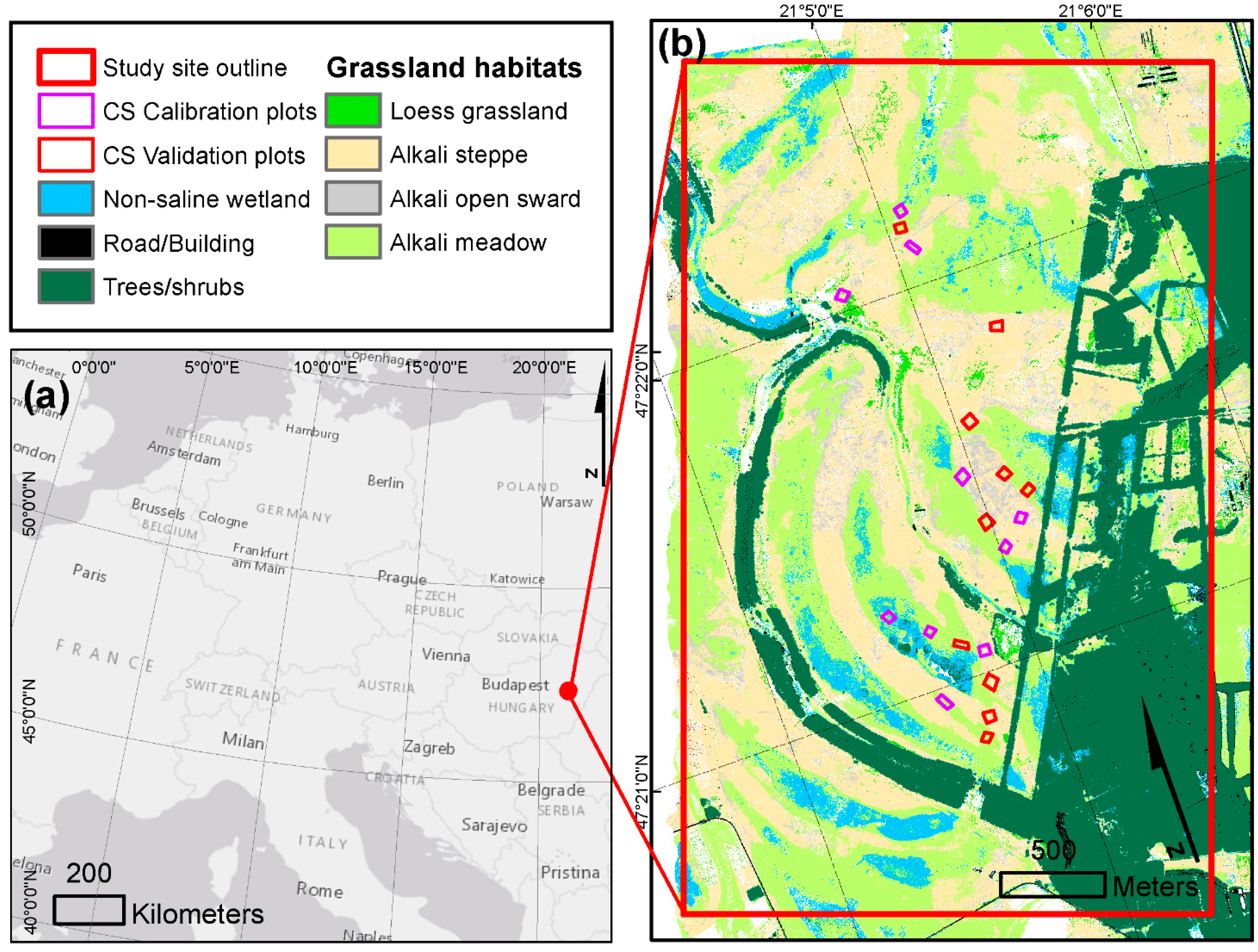
Our study site (Figure 1) is located in Ágota-puszta, a lowland area within the Great Hungarian Plain in Eastern Hungary (N 47°21′, E 21°04′). The region has a continental climate characterized by a mean annual temperature of 9.5 °C and mean annual precipitation of 550 mm [45]. Ágota-puszta is an integral part of the Hortobágy National Park which holds one of the best preserved and largest open landscapes in Europe. It is the part of the UNESCO World Heritage and its whole area belongs to the N2000 network as “Hortobágy Special Area of Conservation” (HUHN20002). Ágota-puszta is characterized by “Pannonic Salt Steppes and Salt Marshes” (1530) N2000 habitat type, with a diverse mosaic of the alkali vegetation types [46]. Grasslands of the study site are mainly grazed by cattle (1.2 livestock unit/hectare/year).
Figure 1. (a) Location of the study site in Central Europe; (b) overview of the study site including land cover, main alkali vegetation classes and CS reference plots.
Remotesensing 07 02991 g001

3.2. Field Data Collection

The field survey was carried out in June 2012. In a layout aiming to cover the whole range of CS and the main alkali grassland types in the area, we designated 20 sample plots of approximately 50 m × 50 m within the habitat Pannonic Salt Steppes and Salt Marshes (Figure 1). We marked the corner points of each plot by a differential GPS [47]. CS was considered according to the assessment scheme to be homogeneous within these plots while each contained a mosaic of various grassland types and associations. Management regime was also homogeneous within each plot while human disturbance varied within them.
Within each single plot, the data collection and N2000 CS assessment was carried out strictly adhering to the instructions of the assessment scheme, which lists 13 parameters to measure or estimate in the field. These parameters are evaluated on a categorical scale of mostly two classes (favorable/unfavorable), in some cases additional sub-parameters are required which are also categorical (e.g., the presence/absence of certain species). Due to these instructions, exact numeric values of CS parameters were not measured, only their respective outcome in terms of categories. This restricted the calibration of our ALS-based CS parameter calculations also to a categorical scale.
Reference polygons of about 5 m × 5 m were collected for calibration and validation of the vegetation classification and feature detection layers, where the vegetation category was noted together with marks of human influence or characteristic microtopography features. Care was taken to select only polygons which were totally homogeneous in terms of vegetation class and other features, including fitting polygon borders to the boundaries of homogeneous patches. The data collection method and layout we applied to alkali grasslands is described in detail in Deák [2]. Furthermore, for this specific study, a total of 123 additional sample polygons of loess grasslands, non-alkali meadows, weed-encroached areas, fields and gardens were mapped together with artificial objects such as roads, buildings and vehicle tracks. The total area of classification references was 0.1 km2 in 364 separate polygons, most of them grouped along 15 field transects from high to low micro-topography. The set of ground truth polygons was split 50:50 into calibration and validation plots.

3.3. Calculation of the N2000 Assessment Scores

We calculated CS scores according to the score sheet of the assessment scheme (see Supplementary Material for full translation). According to this system (slightly different from other national schemes), both positive and negative scores are assigned at plot level based on the CS parameters surveyed in the field. The magnitude of a score is in correlation with the possible impact of the respective parameter on the HQ. For example, if litter accumulation is present in a plot resulting only in a decrease in grass cover, it receives a score of −1, but if it facilitates the spread of invasive species it receives −10. For most variables, the assessment scheme describes a precise threshold (generally a percentage cover) of the studied parameter for the respective scores. Some temporal processes are also included in the assessment parameters, such as changes in the level of litter accumulation on the scale of years. Due to the lack of repetitive surveys across years, we assigned a zero score to all plots for this parameter.
We used the following CS parameters as required by the assessment scheme:
  • Naturalness: this is defined based on the overall status, species pool, structure and management of a site. In Hungary, it is routinely used with a scale ranging from 5 (ecosystem in natural state) to 1 (a severely modified ecosystem). The assessment scheme assigns strong weighting to this parameter: a plot scores +10 points for naturalness values of 4 or 5, 0 points for naturalness of 3 and −5 points for naturalness of 1 or 2.
  • Species density: According to the assessment scheme, “species density “is defined as the variation in the number of species within six 0.5 m × 0.5 m subplots. Alkali grasslands have a very fine mosaic structure and accordingly species density varies considerably even at the 0.5 m scale we investigated. If species density was found unfavorable, a score of −1 was assigned, otherwise 0.
  • Inner patchiness is quantified based on the coverage, species composition, variability and respective area of patches of various vegetation within the assessment plot. This parameter is moderately weighted: +5 points are assigned to the plot if the patchiness corresponds to the typical patchiness of the habitat, −1 point is given if the patchiness is different (higher or lower).
  • Vertical structure for grasslands is defined based on the presence and absence of typical “understory”, “medium level” or “top canopy” grasses and herbs. Weighting of the parameter is moderate: the score of +5 is assigned if the vertical structure corresponds to the typical composition of the habitat, −1 if it is different.
  • Species pool is defined based on the most abundant species and the presence of species typical for Pannonic Salt Steppes and Salt Marshes. The assessment scheme adds strong emphasis to this parameter: +10 points are assigned if the species pool represents the habitat, −5 if the dominant species is not one of those typical for the habitat.
  • Litter accumulation: This parameter is defined based on the amount of dry plant litter within the plot. Strong weighting is applied by the scheme since this is one of the most important potential problems in the studied habitat. +5 points are given if litter accumulation is not present, −1 point for a number of options including high litter cover, litter causing reduction in grass coverage or diversity or accumulation of weeds; finally, −10 points if litter facilitates the spread of invasive species. Here, the negative scores can add up if several negative criteria are fulfilled, so up to −13 points may be reached. In our study site, the grazing regime is the main driver of litter accumulation, with a delicate balance of avoiding both no litter but overgrazing and no overgrazing but eventual litter accumulation.
  • Soil erosion is defined as an estimation of the intensity of ongoing erosion within the plot. The assessment scheme assigns moderate weighting to erosion, giving +5 points if there is no erosion or if it has a positive effect, or −1 for various negative effects. In alkali habitats, natural erosion maintains open alkali sward patches and thus generally has a positive effect in shaping the mosaic pattern of the vegetation.
  • Shrub encroachment is quantified based on an estimate of the coverage of shrubs, their pattern and the list of shrub species observed. The presence of alien invasive shrub species receives a strong negative score (−10), closing of shrub canopy as a consequence of abandonment or disturbance [48] has low weighting (−1 point), and in case the distribution of shrubs is random and contributes to biodiversity [49], a moderate positive score of +5 is assigned.
  • Weed encroachment is defined as the coverage of various weed species, categorized within the assessment scheme. For weed species with different growth strategies, different thresholds are assigned. This parameter is moderately weighed; the scheme assigns +5 points if weed cover is lower than 15% and −1 point if higher. Alkali habitats are less sensitive to weed encroachment as the harsh environment is intolerable for many common weed species.
  • Disturbances are defined as the area ratio of anthropogenic features within the habitat that have a negative effect (incorrect grazing management, vehicle marks, paths, trampling, or rubbish). This parameter is strongly weighted by the scheme: If less than 10% of the plot is affected by any disturbance, +5 points are given, otherwise −1. In our case, the most important disturbances were improper grazing management and additionally treading by vehicles.
  • Future threats are defined as any ongoing processes which might not have an influence at present but can be expected to have a negative effect on the habitat. This is a rather strongly weighted parameter, −5 points are assigned if a future threat is present, +5 if not. The most important future threat identified in the field is the ongoing lowering of the water table and subsequent drying of the site.
  • Animal traces are also defined based on the area affected by animal presence, including grazing, burrowing, rooting, trampling and droppings. Moderate weighting is applied: if more than 50% of the plot is affected, it scores −5 points, otherwise +5. In our study site, which is managed by extensive grazing, the only negative effect observed for some patches was the already mentioned active overgrazing.
  • Landscape context is defined based on the spatial context of the neighboring habitats: whether the habitat patch is neighbored by other natural habitats (local landscape context); whether the nearest similar habitat is within 100 m (wide area context), and finally whether there is a patch of invasive species in the vicinity. This parameter is weighed heavily: the favorable case scores +5, the threat of invasion −10 points. In case of our study site, protected alkali grasslands form a large continuous patch of 20 km2 only broken in some cases by forests, wetlands or roads.
Conservation status is considered favorable (A) if the sum of the positive scores reaches 50 (the maximum is 90), but there are no more than 10 negative scores (which can reach −85 on the scale). CS is unfavorable-bad (C) if there are more than 20 negative scores. Any other cases are in the unfavorable-inadequate category (B).

3.4. Airborne Survey and Primary Data Products

Full-waveform Airborne Laser Scanning of the site was carried out with a Riegl LMS-Q680i scanner, operating in the 1550 nm wavelength. The sensor was deployed on a small fixed-wing aircraft at a flying height of ca. 620 m above ground level, on March 28, 2012 for the leaf-off data and June 13, 2013 for the leaf-on dataset. This resulted in a nominal stripwise echo density of 10 pt/m2 for a total study area of 24 km2. Relative georeferencing accuracy of the strips was validated with the OpalsQuality package script [50], errors were found to be within 2 cm. From the initial georeferenced point clouds, the following datasets were calculated with a spatial resolution of 0.5 m × 0.5 m:
  • A Digital Terrain Model (DTM) was calculated from the leaf-off point cloud using the iterative robust interpolation algorithm [51] in SCOP++ [52]. Based on the DTM, normalized point heights were calculated both from the leaf-off and the leaf-on point cloud by subtracting the ground elevation, and separate output rasters of the interpolated normalized digital surface model (NDSM) and the mean and maximum normalized heights in each raster cell were produced.
  • Surface texture, or roughness, is an important parameter describing the vertical distribution of points within a neighborhood, and is often closely related to vegetation canopy structure [53]. Therefore, rasters were also generated from roughness indices calculated on the normalized point cloud: σz, σ0, and variance.
  • Echo amplitude was calibrated to reflectance, using field spectroscopy measurements of homogeneous targets (asphalt and concrete surfaces) [54]. The mean reflectance of the points within each 0.5 m cell and the variance of the point reflectances with two different kernel sizes (3 × 3 and 5 × 5 pixels) were written to separate output rasters.
  • Echo width is a measure of vegetation canopy structure [25,55], and was calculated separately by online waveform processing for each point by the sensor itself [56]. Mean echo width, maximum echo width from the first echoes and variance of echo width with two different kernel sizes were calculated for each raster.
  • Finally, as a measure of terrain texture, openness rasters (minimum, maximum, average and difference between the minimum and maximum openness) of the DTM [57] were calculated, in order to enhance linear features, sharp edges and local minima and maxima in the terrain.
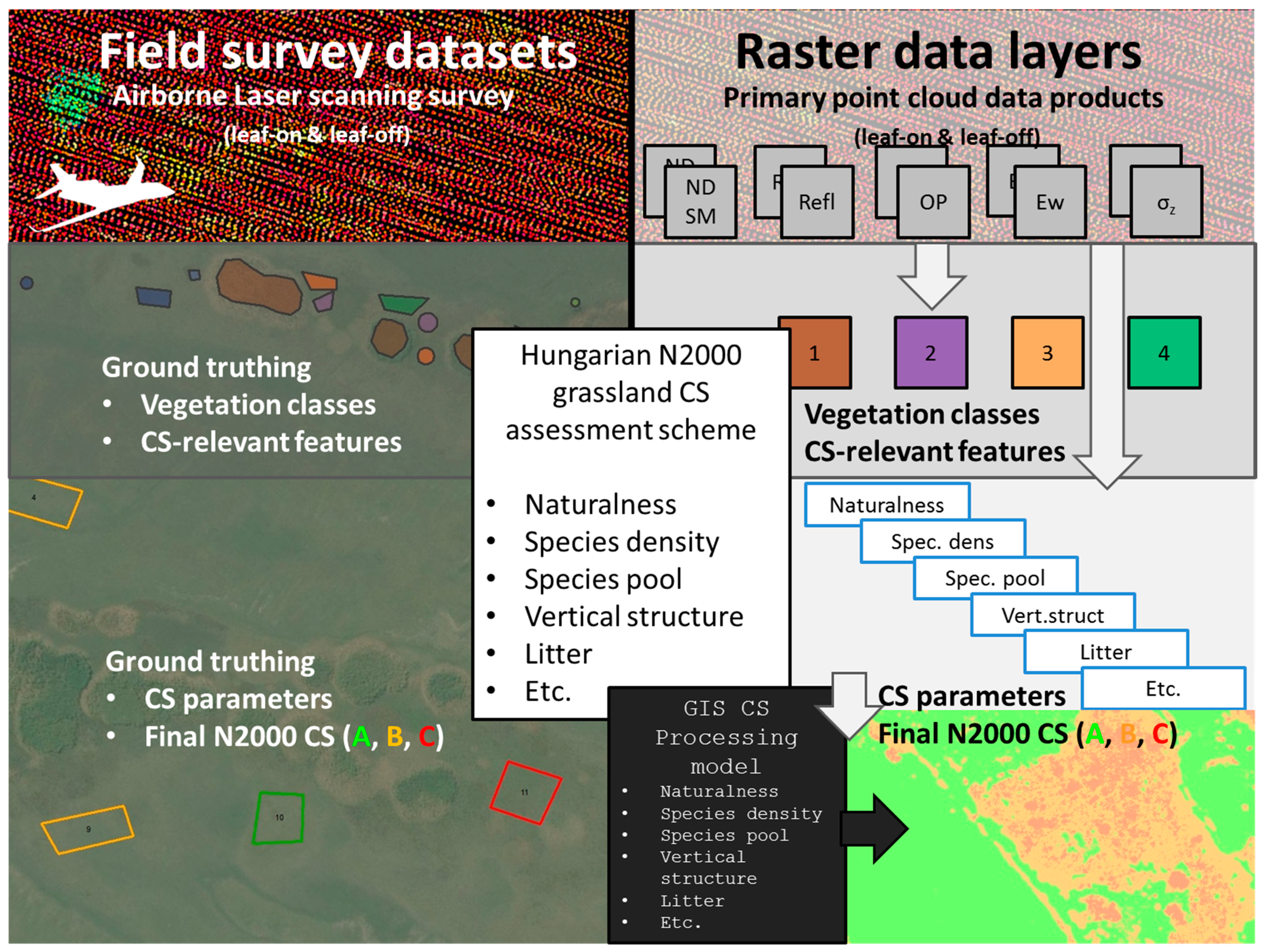
This set of ALS products (Figure 2) was calculated separately for the leaf-off and leaf-on point clouds, and the difference between the leaf-on and leaf-off values was also generated as a separate raster for each product except the DTM. All in all, this resulted in 70 ALS product datasets. All of these were input simultaneously for vegetation classification and feature detection.
Figure 2. Simplified workflow scheme of ALS data processing, vegetation and feature classification, calculation of CS parameter layers and final CS map. Calibration and validation was carried out individually for each processing level.
Remotesensing 07 02991 g002

3.5. Classification of Vegetation and CS-Relevant Features

The dominant vegetation of each pixel was mapped by machine learning classification of the ALS product layers. We exploited the property of our classification method that for each pixel, a probability is assigned to every potential output class and not only the most probable one [58]. In order to map with different levels of detail and also for focusing on different features (vegetation, terrain, human influence), different unique sets of classes of interest were defined (called “scenarios” in the following) and classification carried out for each of these.
We used the Vegetation Classification Studio (VCS) software tool for creating the classifications. This program was built by the authors and is the subject of a separate publication in preparation [59]. An initial description is available under [60] and Zlinszky [61] describes the methodology and processing steps of this software in a case study (without referring to it as VCS).
VCS takes as input vector data describing ground truth polygons for calibration and validation, and a series of raster products of sensor data, in our case those described in Section 3.4. Random forest machine learning [62] is applied in order to classify the output raster, allowing both a fuzzy and a “hard boundary” approach to class membership. Different sets of categories of interest can be processed, and three different output raster maps are produced for each: a hard-boundary vegetation map (mapping 1 pixel to 1 class), a multiband pseudo-image with the probabilities of each class in a separate raster layer for all of its pixels, and finally a color-blended rendering visualizing this fuzzy pseudo-image [25]. Validation of the classification accuracy is an inherent product of VCS and was automatically carried out for all scenarios: a standardized text report of product accuracy including a full confusion matrix [63] and various quality measures (precision, recall, F1-score, Cohen’s Kappa, quantity error and allocation error [64]) was produced, together with a raster map showing the difference in the probabilities of the two most probable classes as a spatially explicit measure of local classification reliability.
In our case, we used a land cover scenario focusing on grassland and non-grassland categories (Supplementary material, Table S3) a set of main vegetation categories based on phytosociological categories which comprise only the main types of alkali grassland (steppe, open alkali swards, and meadow, Supplementary Material Table S4), a set of association-level categories (described in detail in Deák [2] and Borhidi [65]), (Supplementary Material Table S5) and another scenario concentrating on features of human disturbance and weeds (Supplementary Material Table S6) and finally a separate scenario focusing on native and non-native or invasive trees and shrubs (Supplementary Material Table S7).

3.6. Selection and Calibration of CS Parameters

We used a knowledge-based approach for selecting the primary ALS products used for calculating each CS parameter. Based on our understanding of the sensor process, the most appropriate primary ALS products, classifications, and feature probability rasters were selected for each of the CS parameters. The CS parameters are thus also obtained in 0.5 m × 0.5 m pixels. The thresholds determining favorable or unfavorable status were pre-selected based on the requirements of the assessment scheme but were fine-tuned based on the respective parameter values in 10 of the 20 field CS plots (Supplementary Material Table S2). These were selected manually based on their location and attributes, in order to ensure that for each scoring factor and vegetation type, every observed value occurs both in the calibration and validation dataset, and that both calibration and validation polygons are distributed evenly in space. First of all, an optimal distribution of final CS classes was attempted. From the 20 field plots we collected, only one had class C CS and five had A; this determined that the plot with class C was reserved for training, while the two A class plots were assigned to training and three to validation. The next aspect was the distribution of alkali meadows vs. short grass habitats: both A and B status had to be represented for both types, both in training and validation. Finally, care was taken to have all three main types of disturbance (vehicle tracks, overgrazing and undergrazing) as well as undisturbed areas represented for both main alkali vegetation types in the training and validation sets as far as possible.
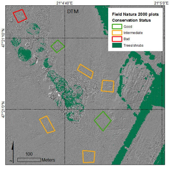
In the next step, with only the calibration CS plots onscreen, the pre-selected direct ALS product or classification output layer was loaded and checked for compliance with the pattern of the respective CS variable of the assessment scheme (Figure 3). We tested direct ALS products such as NDSM height or reflectance, classified rasters representing different habitat features, single-feature and probability layers (bands of the feature probability pseudo-image) and products of spatial analysis operations on these rasters. We aimed to directly use the output of the relevant classification scenario wherever this produced a reasonable pattern compared to the calibration data, and find a meaningful direct sensor data product (see Section 3.4) wherever the classification outputs were not relevant. In some cases, several alternative primary data products were tested. The thresholds between various scores for each CS variable were pre-set manually based on the assessment scheme, and fine-tuned optimizing how the visualized result aligned with the respective scores in the calibration plots (Figure 3). For parameters which had the same value for all plots in the training dataset, the fine-tuning step had to be omitted.
Every CS parameter was validated separately. For each CS parameter output raster, the proportion of pixels was calculated within the respective field CS validation plots that held the same ALS-derived score as assigned during the field survey; therefore, correctly and incorrectly identified plots were detected. Since most parameters had two possible scores, simple majority was used for this. The total ratio of correct/incorrect pixel scores within the validation plots was also calculated for each parameter as a measure of the reliability of the calibration.

3.7. Calculation and Validation of Final CS Scores

The variables listed in Section 3.3 were summed in a single batch script controlling OPALS software modules [50]. Based on the structure of the field mapping instructions where every plot gets separate positive and negative credits, the outputs of this script were also two rasters, one representing the summed positive scores and another the separately summed negative scores for each pixel of 0.5 m × 0.5 m. The resulting output map was masked with non-grassland habitats, and final CS was determined for each pixel of 0.5 m × 0.5 m by comparing these scores to the thresholds laid out in the assessment scheme (Section 3.3). However, these scores could only be validated at the plot level: the ALS-derived positive and negative summed pixel scores were aggregated separately within each CS validation plot. The mean difference and the σMAD of the error distribution between the field-measured and ALS-derived positive and negative scores were calculated as measures of agreement between the field observed N2000 assessment and the ALS-derived CS score (σMAD [66] is a robust estimator for standard deviation also for non-normal distributions). In order to achieve comparability between the 0.5 m final CS raster and the 50 m assessment plots, the pixel-level information had to be scaled up to plot level. Simply taking the most frequent class would not have been a valid representation of the field mapping process: typically, if part of a plot has unfavorable quality, the whole plot will be assigned to B or C class even if the part does not cover the majority of the area. Therefore, a set of rules had to be defined for final CS categorization of the plots based on the ratio of CS classes among their pixels. The calibration polygons which were assigned A, B and C status in the field were respectively merged in a GIS, and the histogram of ALS-based pixel CS scores (A, B and C) generated for each of these, as a way of “signature analysis” for upscaling field observations to plot level. From these signatures, a ruleset for upscaling was generated and applied for gaining plot-level ALS-derived CS scores that are comparable with the field CS categories.
Figure 3. Example of calibrating the scoring layer “species density”. Based on this example, the threshold for favorable species density would be ca. 0.002.
Remotesensing 07 02991 g003
For accuracy assessment, the same relative frequencies of A, B and C class were calculated for the pixels of each validation plot, and the already defined ruleset applied to derive plot-level CS classes based on the ALS data, which were then compared to the field-derived CS category of each plot.

4. Results

4.1. Main Classification Products and Accuracies

  • Land Cover: first of all, the area of the habitat in focus, Pannonic Salt Steppes and Salt Marshes (1530) had to be determined and separated from all other land cover types, which were trees and shrubs, artificial surfaces and non-alkali wetlands. For these categories, producers’ and users’ accuracies based on more than 10,000 validation pixels for each class were typically around 90% (Supplementary Table S3), and Kappa was 0.83, indicating very strong agreement. Non-alkali wetlands proved to be a rather problematic category, on one hand due to the smooth transition towards alkali tall grass wetlands, on the other hand to shrubs with similar height, but even this class had accuracy measures above 65%.
  • Main vegetation categories/alkali subhabitats (Supplementary Table S4): For this scenario, the goal was to separate the three most important vegetation categories of the 1530 habitat type: alkali steppes, open alkali swards and alkali meadows [2]. Loess grasslands, Carex and Juncus dominated wet patches and non-alkali wetlands were added as outgroups together with the category “vegetation background”. The Cohen’s Kappa of 0.625 shows a good agreement between the ALS-derived pixel-level classification and the ground truth training data. Within 1530, dry grassland and wetland categories are rarely confused by the classifier. The main sources of error are discrimination between short grass steppes and open alkali swards, and between tall Carex stands and alkali meadows.
  • Alkali vegetation associations: This was the finest classification level, aiming at identifying each of the alkali grassland and wetland associations. The probabilities assigned to the various associations for each pixel by the random forest classifier were further processed as CS variables. For this set of 16 classes, total accuracy is 62.9%, with a Kappa of 0.579. Most of the misclassifications happened within the main vegetation categories (alkali steppe, alkali sward, alkali meadow and non-alkali wetland) as demonstrated by the error report (Supplementary Table S5).
  • Anthropogenic features and disturbance: The main targets of this scenario were the probability of weed growth and damage by vehicle tracks, each represented by a single-category probability raster during further processing. Weeds had an F1 score of 69%, and rather low quantitative deviation but higher allocation deviation [64]. Unpaved roads were overestimated, with quantitative deviation also high and user’s accuracy of only 48%. Nevertheless, the Kappa of this scenario is 0.77, indicating a strong agreement (Supplementary Table S6).
  • Trees and shrubs: In this scenario, we aimed to identify trees and shrubs and separate alien and native species among them. Accuracies were around 80%, non-native species were slightly overestimated (Supplementary Table S7), Cohen’s Kappa was 0.79. The classified hard boundary raster was used for further processing.

4.2. ALS Products Identified for CS Parameters and CS Scoring

The most important result of manual calibration for various CS parameters was that even for the same ALS products, different thresholds apply for alkali meadows and for the two shorter grass vegetation classes, alkali steppes and open swards. Therefore, before the scores of the CS scheme were calculated, a mask was established separately for tall grass habitats (alkali meadows) and short grass and open habitats (alkali swards merged with steppes), based on the main vegetation classes classification scenario. The mask was processed in a majority filter with a kernel radius of 5 pixels in order to remove some salt and pepper effects that would have propagated through the CS algorithm. Within the two categories of this mask, the following ALS products were selected for representing the CS variables:
  • Naturalness: we used the difference between the leaf-on and leaf-off reflectance. In case of the study site, we observed in the field that the most important factor governing the naturalness of a habitat was the grazing regime: over- or undergrazed patches were in a worse naturalness state than moderately grazed areas. At the 1550 nm wavelength of the ALS sensor, reflectivity of vegetation is proportional to the water content of the cells and thus to the wet or dry biomass [29]. Therefore, if the difference was below 0.2 in meadows or 0.05 in short-grass habitats, this was understood to mean that the amount of standing biomass during the summer grazing season was not much higher or even lower than during the leaf-off season when the grass is typically grazed to the ground. A total of 78.8% of the pixels within the CS validation plots had the correct score based on this calculation. Eight of the plots had high naturalness and more than 80% of their pixels were correctly labeled (Figure 4). Two plots had low naturalness, one of these was incorrectly detected, the majority of the other plot was correct.
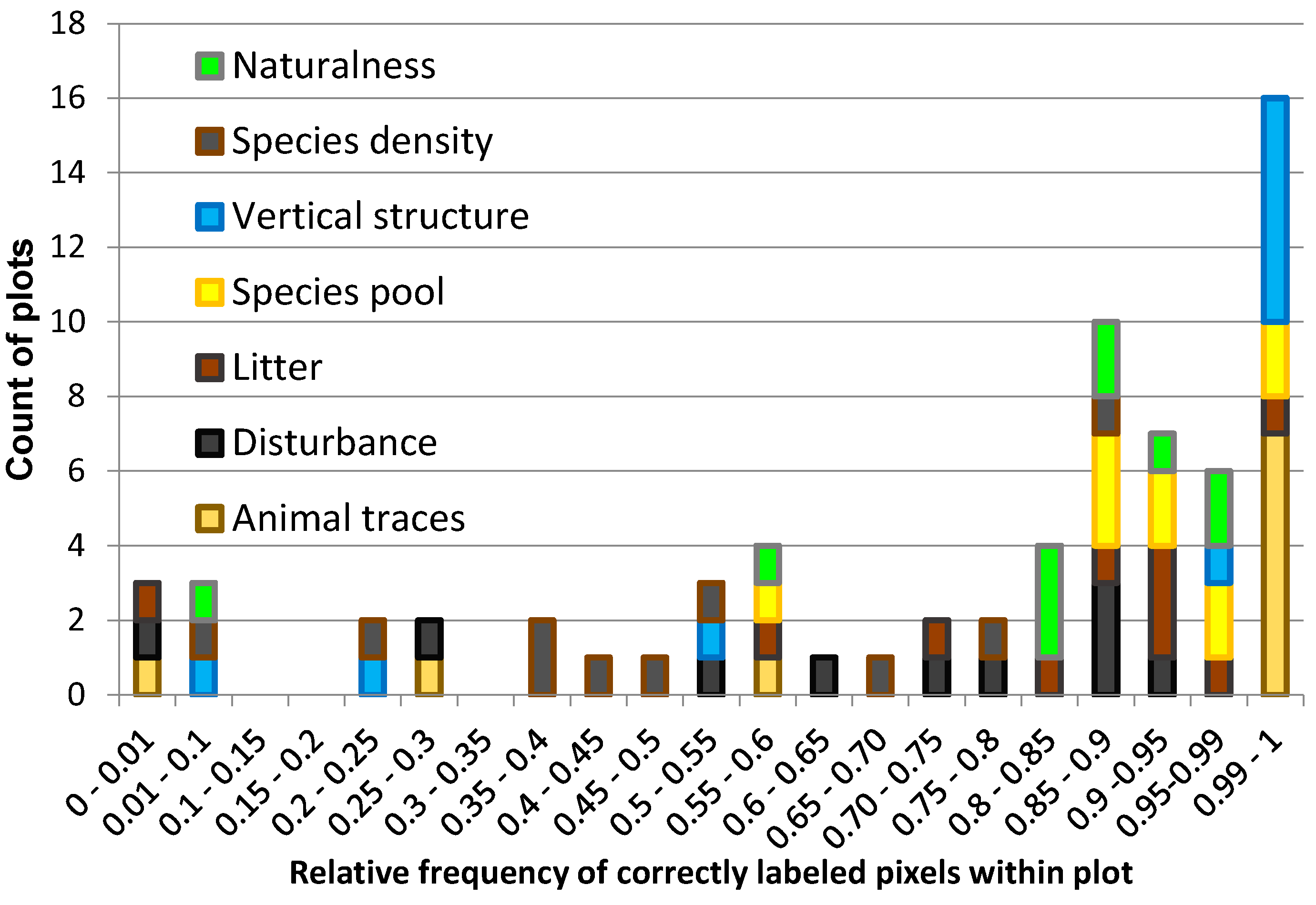
Figure 4. Accuracy assessment of individual CS parameters. Column heights refer to the number of plots having the respective relative frequency of correctly labeled pixels for each CS parameter. Variables where no difference was observed in the field plots are omitted.
Remotesensing 07 02991 g004
  • Based on the Spectral Variation Hypothesis [67], species density was represented with the variance of the leaf-on point reflectance within a pixel. To follow the different characteristic scales for long and short grass habitats, a 5 × 5 cell kernel was applied for meadows and a 3 × 3 cell kernel for steppe and sward, but the threshold separating favorable and unfavorable species density was 0.001 in each case. 47.2% of all the pixels in the CS validation plots had the correct score, with only a single plot being more than 80% correct and half of the validation plots having more incorrect species density scores than correct ones. Two plots had unfavorable species density; the majority of the pixels in one of them was correctly identified.
  • Inner patchiness: All plots showed constant favorable patchiness; therefore, we assigned the same score to all alkali habitats (based on the grassland habitat mask). Based on the land cover scenario, this mask has accuracies above 90% (Supplementary Table S3).
  • Vertical structure: The difference between leaf-on and leaf-off maximum normalized point height was identified as a proxy for vertical structure. We applied a threshold of −0.15 m separating favorable and unfavorable conditions. A total of 82% of the investigated pixels were correctly classified, six plots were over 99% correct, but two (including the single one with unfavorable vertical structure) had less than 50% correct pixels.
  • Species pool: We used the summed probability of alkali grassland associations (from the association-level scenario output) as a proxy for this variable. These values were summed separately for the associations corresponding to meadows and short grasslands/open swards, with unfavorable species pool assigned to a pixel if the probability of it belonging to any of these was below 50% and favorable if above this limit. Only one calibration CS plot and no validation plots had unfavorable species pool, which explains the observed performance of this ALS-based indicator: 91% of all validation pixels were labeled correctly, with no misclassified plots.
  • Litter accumulation: The difference in leaf-on and leaf-off reflectance proved to correspond to the pattern in the litter accumulation of our calibration plots (threshold >0.3 unfavorable). The various levels of negative effects of litter could not be resolved from our sensor data. We assigned either +5 or −1 point to a pixel based on litter accumulation, and classified only the quantity of litter but not its effect (see Section 3.3) Four validation plots had favorable litter quantity and six unfavorable, and all but one (unfavorable) were correctly detected with 79% of all the validation pixels well identified.
  • Soil erosion: All field plots received favorable scores for this factor, since only positive effects of erosion were observed in the site. Therefore, we simply assigned the favorable value to all pixels belonging to the alkali grassland habitats. The accuracy of this indicator is the same as the accuracy of grassland masking.
  • Shrubs: None of our field plots contained any shrubs, but both native and alien invasive shrubs were present in the site. Following the assessment scheme, we used the scenario “trees and shrubs” with a morphological opening operation [68] to identify dense stands. This was compared with the class “alien invasive trees/shrubs” to identify separately the “low density”, the “dense native” and the “dense alien invasive” classes. Since this indicator directly relies on the output of the tree/shrub classification layers, its accuracy is at or above 65% (Supplementary Table S7).
  • Weeds: We used the single-band weed probability layer from the “anthropogenic features and disturbances” scenario. The threshold for unfavorable presence of weeds was assigned to be 65% probability in absence of more detailed calibration data. Again, the reliability of this indicator could not be tested; the accuracy of the weed probability layer is quantified within the respective classification scenario (Supplementary Table S6).
  • Disturbances: For grazing regime, difference in maximum normalized height was used again for meadows, with differences below −0.15 representing overgrazing and above −0.02 representing undergrazing and litter accumulation. In short grasslands, overgrazing is less of an issue as the standing crop is low anyway. Again, we used the difference in leaf-on and leaf-off reflectance and the already established threshold of <0.3 for undergrazing. As for treading by vehicles, we took the probability of the class “unpaved road” from the “anthropogenic features and disturbances” scenario, which included established field roads and also individual vehicle tracks, and set a threshold of 65% probability to identify any pixel where tracks can be suspected. Six of our CS validation plots received a negative score for disturbance while four were in favorable state; all except one (unfavorable) were correctly identified. A total of 64% of the pixels within the total area of the validation plots was labeled correctly, and four plots had more than 85% correctly labeled pixels (two in favorable and two in unfavorable status). According to the assessment scheme, a plot already qualifies as disturbed if 10% of its area is affected, which explains some of the plots with lower proportions labeled correctly, but not the single case of a disturbed plot where less than 1% of the pixels were correct.
  • Future threats: The gradual lowering of the water table as the most important future threat has a long-term dimension in time and therefore cannot be identified by two remote sensing surveys within a few months. However, it correlates closely with terrain elevation: lower lying areas are less threatened. The DTM was used as a source dataset and since all the calibration/validation polygons were estimated in the field to be affected by this risk, only the areas lying below the lowest calibration plot (127.25 m) were considered to be unaffected, which are nearly all non-alkali wetlands in our site. The accuracy of this parameter could not be tested either, but since the accuracy of the DTM is within 5 cm, the area of the study area within ±2.5 cm of this threshold was calculated, which is 5% of the total area. No part of the CS calibration or validation plots lies in this elevation interval.
  • Animal traces: active presence and overgrazing of livestock was calculated from the difference in leaf-on and leaf-off maximum normalized height, but assigned a slightly different threshold of −0.17 compared to the threshold for litter accumulation in accordance with the scheme. One of the CS validation plots was in an unfavorable status in terms of animal traces, this plot had no correctly labeled pixels, and two other plots also had less than 60% correct pixels. Therefore, the overall ratio of 82% correctly labeled pixels within the CS validation plots is an overestimation of performance.
  • Landscape context: The CS scheme defines two levels of landscape context. Therefore, we counted for each pixel the amount of alkali grassland pixels in its neighborhood with two different kernels: 15 × 15 pixels representing the neighboring environment (with a threshold of 220 pixels representing a large number of similar neighbors) and 100 × 100 pixels to imitate the rule of “closest similar habitat is not more than 100 m away”. The accuracy of these indicators corresponds to the accuracy of the alkali habitat masking in the land cover scenario, which is 95% (Supplementary Table S3).
The assessment scheme deals separately with the summed positive and negative scores of each plot, which, however, are the results of the same mapping process. For each parameter, either a positive or a negative score is assigned to the plot, while the final score is derived by comparing both the positive and the negative scores to pre-set thresholds (Section 3.3). The sum of positive and negative scores is not used by the assessment scheme.
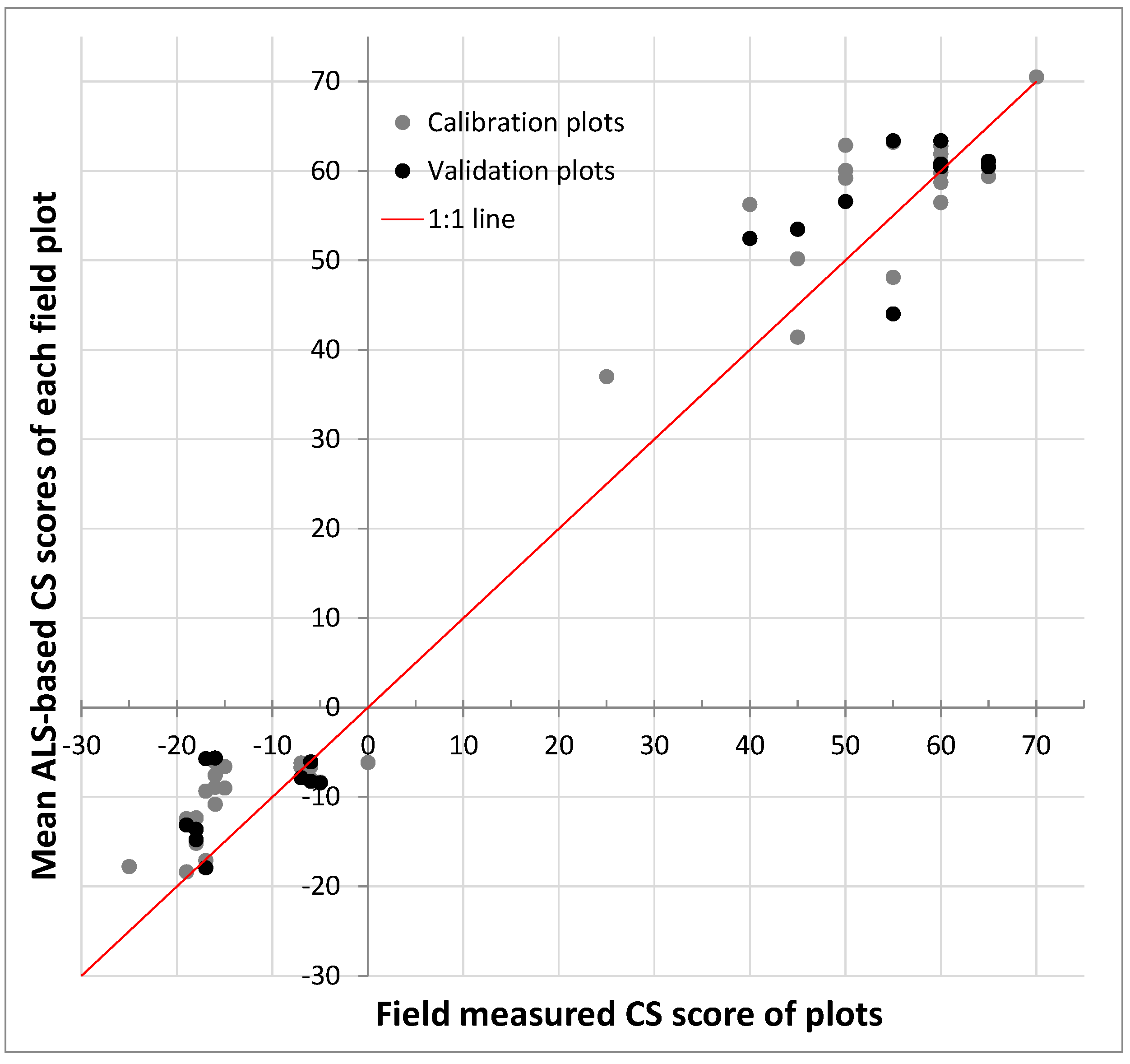
Therefore, the effect of the weighting and evaluation scheme on the final score with respect to the performance of the individual CS parameters was investigated by plotting the ALS-derived summed positive and summed negative CS scores against the respective field-measured scores (Figure 5). For this, the mean of the pixel positive and negative scores within each plot were taken, resulting in 20 positive and 20 negative points in the scatterplot, 10 each from the calibration and validation datasets.
Figure 5. Scatterplot of plot-level positive and negative CS score from field mapping vs. ALS-based positive and negative CS score averaged for each plot.
Remotesensing 07 02991 g005
The study site held alkali habitats in good natural state; therefore, six of the 13 parameters we investigated held constant scores of +5, explaining why no points are between the origin and the (30; 30) point. The combined error distribution of the positive and negative scores shows a median bias of −2.33 and has a σMAD of 6.50. This shows that the ALS-based HQ evaluation script performed adequately not only on a categorical scale of three classes but also on a more detailed numeric scale. Apparently, some of the parameters that were inaccurately detected had low weighting, while others that were reliably detected were emphasized by the assessment scheme.

4.3. Final CS Modeling Algorithm and its Performance
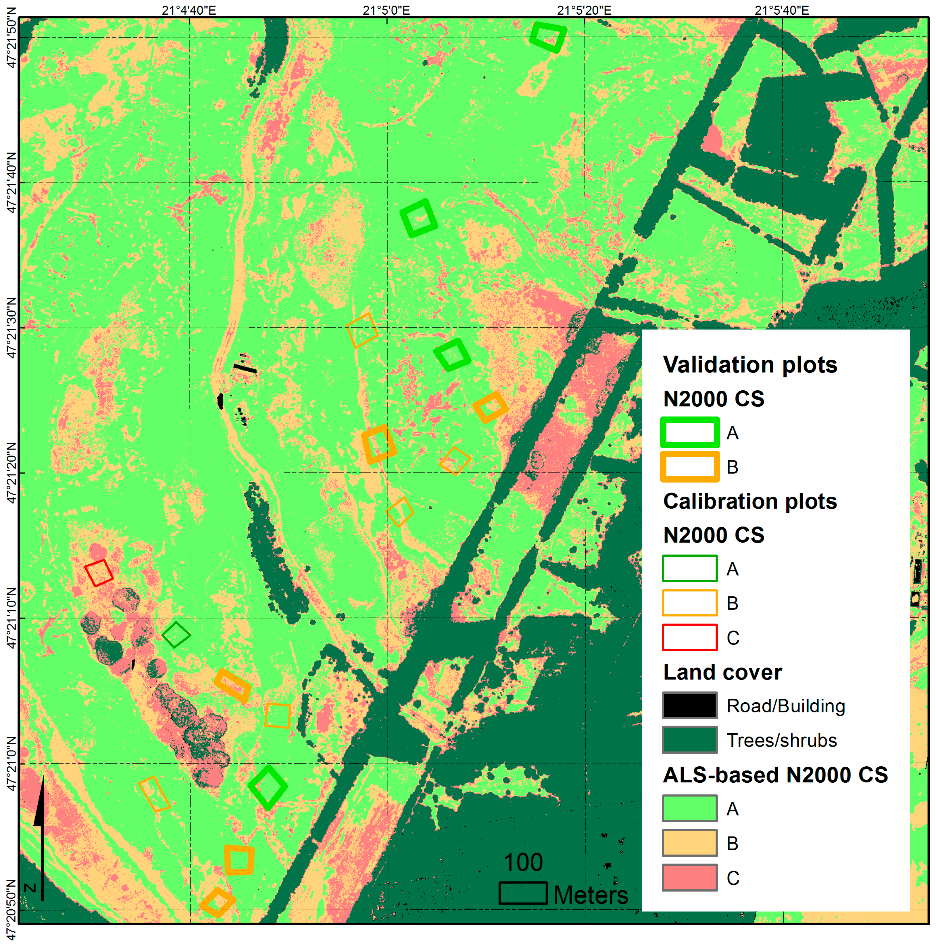
The resulting map (Figure 6) shows that the ALS-mapped CS mostly matches the scores of the plots, but there is considerable heterogeneity within the 50 m × 50 m ground mapping units. Due to the high weighting of the parameter disturbance, CS mostly follows the pattern of this parameter, with roads and tracks showing up as patches of worse CS than their neighboring areas. The most important source of error in the pixel-level CS seems to be the misclassification of alkali erosion features as vehicle tracks and, consequently, the labeling of these natural features as human disturbance. Another important observation is that although the overwhelming majority of the surveyed field CS plots belong to the class B, most of the study area is shown by the pixel-level map to belong to A.
Figure 6. Cutout of the final CS map, showing some of the calibration and validation plots and the fine-scale CS patterns within them.
Remotesensing 07 02991 g006
The histogram resulting from plot-level CS signature analysis (Figure 7) shows that a plot assigned to class A in the field could still have about 10% of B and 7% of C within it. It was also clear that the majority of pixels within plots assigned to B belong to class A, with about 30% of the pixels belonging to B and some presence of C. Similarly, if a reference plot had at least 20% of C, the overwhelming majority was B and no A was present, the plot was observed in the field as having C status. Based on these observations and investigation of the individual ratios of A, B and C in the calibration plots, the following ruleset for upscaling from pixel level to plot level was defined:
  • If a plot has more than 70% pixels in class A the plot qualifies as A.
  • If A is below 10% and C is above 25% then the plot belongs to C.
  • In all other cases the plot qualifies as B.
For eight of the 10 plots, the ALS-based plot-level CS class matched the field observation (Kappa of 0.60). The correctly identified plots include steppes and meadows of both favorable (A) and unfavorable-inadequate (B) quality.
Figure 7. Frequency of 0.5 m ALS-derived pixels representing each HQ class within the summed field calibration plots of each respective category.
Remotesensing 07 02991 g007

5. Discussion

5.1. Reference Data Availability

At the raster resolution we used, each ALS product raster cell is calculated from several laser pulses within the pixel. Exceptions to this are the various roughness measures, which used the eight nearest neighbor points within a radius of 2 m and the reflectance and echo width variance products. This independence allowed us to treat pixels as individual samples for calibration and validation of vegetation and feature classification. Nevertheless, the randomized 50:50 split between training and validation data was carried out at field polygon level. For nearly all classes, this resulted in thousands to ten thousands of training and validation pixels for classification from several independent plots, and resulted in good classification accuracies.
One of our most important objectives was to train and evaluate our model with field data collected strictly adhering to the assessment scheme. A result of this is the limited number and range of CS field plots available, since a full N2000 survey had to be carried out in each location. Ideally, several field operators would have been needed and the actual value (not just the class) of all CS parameters would have had to be measured in a layout similar to Spanhove [37]; however, this study mapped more than 10% of their study area for ground truths while we mapped about 4%.
In case of the CS parameters within our study, selection was done manually in order to find the best possible combination within our limited possibilities. Our experience during this process was that a representative combination of parameters within both the training and validation plots could best be achieved with a 50:50 split. Manual training and evaluation was carried out at the level of individual plots, aggregating information from the ALS-derived raster pixels within them.
Random selection of training and validation plots was out of question since it could have resulted in only a single value for either calibration or validation for most parameters. Leave-one-out cross validation would have required individual training of the manual calibration and upscaling process several times and was therefore not feasible for the level of CS parameters and final plot-level status.

5.2. ALS Data and its Effectiveness for Quantifying All CS Relevant Parameters for N2000: Errors, Uncertainties, Accuracies

A previous ALS-based grassland classification study has reached accuracies very similar to those we achieved for the vegetation categories level [25]. Vegetation classification is the basis of all biodiversity and habitat quality maps, and our results are in accordance with previous ALS-based grassland classification studies showing that high resolution, full waveform, radiometrically calibrated multi-temporal ALS data in combination with a state-of-the-art machine learning algorithm is powerful enough for efficient vegetation mapping with this level of detail.
There are several examples in the literature of HQ-relevant parameters of grassland vegetation being quantified from remote sensing data [31,34,69]; in most cases, the results are based on dedicated experiments focusing on the full range of a single variable quantitatively measured in the field. In our case, this was not possible: most of the properties of the habitats were only assessed on a categorical scale. However, we aimed at representing all of them in a CS model based on ALS data.
The indicator data products we propose all have plausible physical and botanical explanations. It is already established for grasslands that very small differences between the values of certain ALS products (e.g., a couple of centimeters in normalized point height) can consequently represent real differences in vegetation properties [25]. The CS parameters can be assigned to distinctive groups based on their observed quality.
For the parameters “litter” and “disturbances”, the field data range was sufficient to validate the algorithm, which was found to perform reliably. These parameters are partly derived from the same data product (the difference between leaf-on and leaf-off reflectance), but disturbances also include a single-feature probability product.
For “patchiness”, “species pool”, “soil erosion”, “shrubs”, “landscape context” and “future threats”, all validation plots held the same score. Therefore, the accuracy of the parameters could not be directly assessed. However, since these were directly derived from classification products, their accuracy is well quantified and satisfactory. Each of these variables was separately determined by machine learning on the primary ALS products, and therefore independent of specific expert expectations.
The parameters “naturalness”, “vertical structure” and “animal traces” repeat the same error pattern: all cases of favorable status are correctly detected, but only one or two plots are unfavorable and one of these is always misidentified. Here, the distribution of reference data presents a limitation to checking the quality of these parameters. The difference between leaf-on and leaf-off normalized point height or reflectance is also the basis for these parameters, but the individual thresholds are different.
Finally, for “species density”, the physical explanation of the selected ALS product is plausible, but the accuracy of parameter estimation is unsatisfactory. Since species density has a rather low weighting, the low accuracy of this indicator did not have a strong influence on the final CS score or classification.
Several variables that the Hungarian N2000 scheme evaluates separately (e.g., litter accumulation, effect of animals, vertical structure) proved to be very closely related to each other in our study site due to the management regime and characteristics of the alkali steppe landscape. In these cases, we did not try to use independent ALS-based datasets for these variables either. This is in line with the findings of Spanhove [37], who also conclude that coarse-scale HQ parameters can overrule the effects of finer-scale variables.
The calculation of single-class probability rasters or hard-boundary classified rasters also proved to be highly useful. The probability of weeds and of vehicle tracks and the coverage of shrubs was directly used as an indicator compatible with field observations. The output reports and probability difference maps of the VCS for each scenario provide a detailed understanding of the accuracies to expect from these datasets.
We have shown that ALS can deliver adequately reliable indicators for nearly all the variables that are required by the assessment scheme. Even if some of these could probably be better represented from other sensors, the ALS-derived values proved to be robust and accurate enough for use in a CS model that integrates them all to a final score. For such an application and given sufficient field calibration data, ALS as a standalone sensor can deliver all the information needed.

5.3. Mapping Natura 2000 Conservation Status: Errors, Uncertainties, Accuracies

Within the 10 validation plots, the two cases of incorrect CS assignment and/or upscaling are plots dominated by short grass habitats, where the main cause of disturbance is improper management. Apparently, the level of litter accumulation is difficult to determine by ALS in short grass steppes, and our accuracies for identifying vehicle tracks are rather low compared to other classes. The weighting of this variable (disturbance) means inaccuracy here easily results in misclassification of CS.
To our best knowledge, no remote sensing-based N2000 CS study has been published where accuracy of CS categorization is evaluated against plot-level independent references. Therefore, these figures can only be compared with the expected reliability of the field-based method, which is around 80%–85% at the level of habitat classification [35,70,71]. In many cases, a field campaign includes disputed or uncertain decisions, and a lot of extrapolation to site level is done, which does not necessarily happen in our sensor-based CS map which covers the full site.
The similarity achieved between field-measured and ALS-based positive and negative CS scores compares favorably to the accuracies reached by some grassland remote sensing studies that aimed to quantify only a few variables or a single one [28,29,32]. Part of this high reliability can be explained by the facts that the assessment scheme integrates several variables, and that we used mean values aggregated across a larger area: both of these reduce the effect of random noise. Meanwhile, we excluded the time-series variables from both the field and the ALS mapping scheme, but this did not have a major negative effect on score accuracy. Since we followed the assessment scheme with the CS processing model, we believe this figure is truly an indication of how our method compares to field-based N2000 Monitoring.

5.4. The HQ/CS Model Directly Based on the Hungarian N2000 Grassland Evaluation Scheme

GIS-based HQ maps rely on a model of HQ that includes the relative importance of all the involved factors and is built based on ecological knowledge. However, since many different definitions of HQ exist [72] and the importance of various HQ factors is by no means fully resolved, these HQ models are always a subject of dispute. A HQ model can be built with a specific application in mind (restricting transferability), it can be created on a statistical basis, automatically weighting the inputs to produce the best agreement to reference data [44], or, as we did, a widely accepted HQ/CS model finalized by a consensus of the relevant scientific community can be taken and directly used. This also has its risk since the model was created with a different application in mind, and is only feasible if a close representation between its required input datasets and the products of the sensor can be found.
In our case, this definitely proved feasible. All relevant CS variables were quantified and the selection of variables, their weighting and integration follows the Hungarian Natura 2000 grassland evaluation scheme very closely.

5.5. Method for ALS-Assisted N2000 CS Mapping of Alkali Grasslands

We propose a method combining various approaches to remote sensing of vegetation: hard boundary classification, class probabilities calculated with a fuzzy approach, and primary point cloud products that represent different properties of vegetation. Raster algebra is the platform where all these input features are integrated and compared. This means that the system is compatible with any sensor, or any dataset that may be rasterized as an information layer [19]. From a N2000 perspective, most of the site belongs to a single habitat class, but in order to mimic the “ecological common sense” applied by the field scientists, we separated steppes and meadows and applied different thresholds and sometimes even different ALS data products to quantify the same variables for these two classes. This has delivered a decisive improvement in accuracy compared to our earlier attempts where this separation was not included [61].
Our approach relies on several levels of training and validation data and therefore intensive fieldwork, given its multiple processing levels and the large number of features involved. On the contrary, in a typical N2000 monitoring setting, an expert for the habitat category 1530 would visit the site and collect field data from one or a few plots based on the assessment scheme. This amount of information may be sufficient for international policy, but local-level conservation management is in need of more detailed knowledge. Our method provides a resolution comparable to the typical patch size in the target habitat, and full coverage of the site, while completely retaining compatibility with the field HQ survey results.

5.6. Data Products of the Assessment and Their Use in Conservation

The by-products of the processing chain including the classified vegetation maps and various CS-relevant features were often observed during visual quality control to be accurate representations of the situation in the field. However, this might only work on a categorical scale. Their applicability for true quantitative representation of biophysical variables remains to be tested.
Nevertheless, they are already expected in their current form to be useful for conservation management, but also for scientific purposes: shifting boundaries of associations (e.g., due to climatic or management changes) can be identified, the extent of major risks calculated, habitats for specific animal species located. The scoring system allows checking how the final categorization is calculated for each pixel or any region of pixels specifically, and therefore also allows evaluation of why that particular score is assigned. Contrary to sample-based field results, the interpretation of such maps is often very intuitive, even for non-specialists. Nevertheless, they do not provide a substitute for field surveying; they can rather serve as a basis for planning future field campaigns and upscaling the observations made in the field.
Whether field or sensor-based, the final scores should be treated carefully due to the generalizations of the Hungarian N2000 grassland assessment scheme across various types of grasslands. In alkali landscapes over- or undergrazing, (the most frequent disturbance observed) generally has a short-term effect, as alkali habitats can regenerate after these disturbances very well. Even over- or undergrazed areas contribute to habitats for several animal taxa, such as birds or insects [73]. On the other hand, damage caused by vehicles (which is weighted equally to improper management) can be a major problem for the habitats of the study site. The special soil conditions conserve tracks of vehicles for decades as long-lasting scars in the landscape.
The heterogeneity of the site in terms of CS as shown by the map is also informative, and contests the assumption of the assessment scheme that CS is homogeneous within 50 m × 50 m plots. While field-based assessment only gives information on the location of the plot and its HQ, with sensor data covering the whole site, it is possible to tell where the areas of favorable, unfavorable-inadequate and unfavorable-bad status are.

5.7. Outlook

Our study has shown that area-covering CS/HQ mapping by ALS is possible, and directly comparable with the local N2000 field mapping scheme. While adaptation to other sites remains to be tested, in areas of highest conservation priority and difficult field access, this may well be the only way to gain a complete overview of habitat conditions.
Given the increasing ALS coverage of Europe and North America from national campaigns, the next step would be to test a similar workflow on larger areas with lower density point clouds. Alternative models for HQ/CS that are more adapted to remote sensing while still comparable with the N2000 scheme might also be developed, and would probably result in higher accuracies.
Comprehensive and robust information on the status of biodiversity, ecosystems and ecosystem services is recognized as a necessary condition of implementing the EU Biodiversity strategy [10,74]. The insufficiency of information on spatial patterns of biodiversity is also identified as a major difficulty in addressing the global biodiversity crisis [75]. Hopefully, with mapping workflows similar to what we present here, this data gap can at least partially be filled, providing measurable indicators for national and international biodiversity policy. It is expected that with increasing ALS data coverage, decreasing costs for sensor campaigns and novel sensor platforms such as UAV-s, ALS will prove to be a cost-effective solution for vegetation mapping in grasslands.

6. Conclusions

We developed a new method for mapping Natura 2000 Conservation Status from Airborne Laser Scanning (ALS) data in Pannonic Salt Steppes and Salt Marshes, adhering during the data processing exactly to the official Conservation Status interpretation manual defined for field surveys. Twelve of the 13 parameters requested by the local Natura 2000 assessment scheme can be derived from ALS with sufficient accuracy. The final accuracy of the end product, validated against independent field data, is 80% (Kappa 0.6). The method is compatible with other sensor datasets and is expected to allow transfer to other sites.
Conservation status was never before mapped by a single-sensor dataset and a processing scheme that strictly followed the national Natura 2000 manual. We managed to map Natura 2000 conservation status from the ALS data and a set of ground references, quantifying all relevant parameters and taking them into account. Our results show that operational use of remote sensing for Natura 2000 processing is feasible and can be compatible with the current, field-based approach.

Supplementary Materials

Supplementary materials can be accessed at: https://www.mdpi.com/2072-4292/7/3/2991.

Acknowledgments

The data collection and research leading to this study was funded by the ChangeHabitats2 Marie Curie IAPP project (Contract No. 251234). We gratefully acknowledge the work of Cici Alexander who calculated many of the initial ALS data products. Background map of Europe for Figure 1a and the orthoimage used as a background in Figure 3 are basemaps of ESRI ArcGIS, with data owned by ESRI, DigitalGlobe, GeoEye, i-Cubed, EarthStar Geographics, CNESAirbus DS, USGS, AEX, GeoMapping, Aerogrid, IGN, IGP, Swisstopo, DeLorme, MapMyIndia, OpenStreetMap contributors, and the GIS user community.

Author Contributions

András Zlinszky coordinated teamwork, wrote the processing script for calculating CS scores and variables, and performed accuracy assessment. Balázs Deák collected the field data, helped refine the calculations and link ALS products to CS variables. Adam Kania coded and operated Vegetation Classification Studio; Anke Schroiff contributed to field mapping and the development of the classifier; Norbert Pfeifer led the study and also helped to connect sensor data products to ecological variables. All authors contributed to writing the manuscript text and graphics.

Conflicts of Interest

The authors declare no conflict of interest.

References

  1. European Commission DG Environment. In Interpretation Manual of European Union Habitats; EUR 28; Nature and Biodiversity: Bruxelles, Belgium, 2013; p. 146.
  2. Deák, B.; Valkó, O.; Alexander, C.; Mücke, W.; Kania, A.; Tamás, J.; Heilmeier, H. Fine-scale vertical position as an indicator of vegetation in alkali grasslands—Case study based on remotely sensed data. Flora 2014, 209, 693–697. [Google Scholar] [CrossRef]
  3. Valkó, O.; Tóthmérész, B.; Kelemen, A.; Simon, E.; Miglécz, T.; Lukács, B.; Török, P. Environmental factors driving vegetation and seed bank diversity in alkali grasslands. Agric. Ecosyst. Environ. 2014, 182, 80–87. [Google Scholar] [CrossRef]
  4. Deák, B.; Valkó, O.; Tóthmérész, B.; Török, P. Alkali marshes of Central Europe—Ecology, management and nature conservation. In Salt Marshes—Ecosystem, Vegetation and Restoration Strategies; Shao, H.-B., Ed.; Nova Science Publishers: New York, NY, USA, 2014; pp. 1–11. [Google Scholar]
  5. Kelemen, A.; Török, P.; Valkó, O.; Miglécz, T.; Tóthmérész, B. Mechanisms shaping plant biomass and species richness: Plant strategies and litter effect in alkali and loess grasslands. J. Veg. Sci. 2013, 24, 1195–1203. [Google Scholar] [CrossRef]
  6. Deák, B.; Valkó, O.; Török, P.; Tóthmérész, B. Solonetz meadow vegetation (Beckmannion eruciformis) in East-Hungary–an alliance driven by moisture and salinity. TUEXENIA 2014, 34, 187–203. [Google Scholar]
  7. European Commission. Council Directive 92/43/EEC of 21 May 1992 on the conservation of natural habitats and of wild fauna and flora. Official Journal of the European Union 1992, 206, 7–50. [Google Scholar]
  8. Weber, N.; Christophersen, T. The influence of non-governmental organisations on the creation of Natura 2000 during the European Policy process. For. Policy Econ. 2002, 4, 1–12. [Google Scholar] [CrossRef]
  9. European Topic Centre on Biological Diversity. In Habitats Directive Article 17 Report (2001–2006) Data Completeness, Quality and Coherence; ETBD: Paris, France, 2008; p. 24.
  10. European Commission. The EU Biodiversity Strategy to 2020; DG Environment, Publications Office of the European Union: Luxembourg, Luxembourg, 2011; p. 28. [Google Scholar]
  11. Vanden Borre, J.; Paelinckx, D.; Mücher, C.A.; Kooistra, L.; Haest, B.; de Blust, G.; Schmidt, A.M. Integrating remote sensing in Natura 2000 habitat monitoring: Prospects on the way forward. J. Nat. Conserv. 2000, 19, 116–125. [Google Scholar]
  12. Simonson, W.D.; Allen, H.D.; Coomes, D.A. Applications of airborne LiDAR for the assessment of animal species diversity. Methods Ecol. Evol. 2014, 5, 719–729. [Google Scholar] [CrossRef]
  13. Asner, G.P.; Hughes, F.R.; Mascaro, J.; Uowoli, A.L.; Knapp, D.E.; Jacobson, J.; Kennedy-Bowdoin, T.; Clark, J.K. High-resolution carbon mapping on the million-hectare Island of Hawaii. Front. Ecol. Environ. 2011, 9, 434–439. [Google Scholar] [CrossRef]
  14. Corbane, C.; Lang, S.; Pipkins, K.; Alleaume, S.; Deshayes, M.; Millán, V.E.G.; Strasser, T.; Borre, J.V.; Toon, S.; Michael, F. Remote sensing for mapping natural habitats and their conservation status—New opportunities and challenges. Int. J. Appl. Earth Obs. Geoinf. 2014, 37, 7–16. [Google Scholar] [CrossRef]
  15. White, R.P.; Murray, S.; Rohweder, M. Pilot Analysis of Global Ecosystems—Grassland Ecosystems; World Resources Institute: Washington, DC, USA, 2000; p. 81. [Google Scholar]
  16. Veen, P.; Jefferson, R.; de Smidt, J.; van der Straaten, J. Grasslands in Europe of High Nature Value; KNNV Publishing: Zeist, The Netherlands, 2009; p. 320. [Google Scholar]
  17. Burai, P.; Deák, B.; Valkó, O.; Tomor, T. Classification of herbaceous vegetation using airborne hyperspectral imagery. Remote Sens. 2015, 7, 2046–2066. [Google Scholar] [CrossRef]
  18. Schuster, C.; Schmidt, T.; Conrad, C.; Kleinschmit, B.; Förster, M. Grassland habitat mapping by intra-annual time series analysis—Comparison of RapidEye and TerraSAR-X satellite data. Int. J. Appl. Earth Obs. Geoinf. 2015, 34, 25–34. [Google Scholar] [CrossRef]
  19. Buck, O.; Millán, V.E.G.; Klink, A.; Pakzad, K. Using information layers for mapping grassland habitat distribution at local to regional scales. Int. J. Appl. Earth Obs. Geoinf. 2015, 37, 83–89. [Google Scholar] [CrossRef]
  20. Reese, H.; Nyström, M.; Nordkvist, K.; Olsson, H. Combining airborne laser scanning data and optical satellite data for classification of alpine vegetation. Int. J. Appl. Earth Obs. Geoinf. 2014, 27, 81–90. [Google Scholar] [CrossRef]
  21. Bork, E.W.; Su, J.G. Integrating LiDAR data and multispectral imagery for enhanced classification of rangeland vegetation: A meta analysis. Remote Sens. Environ. 2007, 111, 11–24. [Google Scholar] [CrossRef]
  22. Ichter, J.; Evans, D.; Richard, D. Terrestrial Habitat Mapping in Europe: An Overview; TH-AK-14-001-EN-N; European Environmental Agency: Luxembourg, 2014; p. 152. [Google Scholar]
  23. Corbane, C.; Deshayes, M.; Elena, G.M.V.; Strasser, T.; Vanden Borre, J.; Spanhove, T.; Förster, M.; Lang, S.; Pernkopf, L. Deliverable 3.2, Technical Synthesis on the Possibilities and Limits of RS for Mapping Natural Habitats; Institut National de Recherce en Sciences et Technologies pour l’Environement et l’Agriculture: Montpellier, France, 2013; p. 82. [Google Scholar]
  24. Ward, R.D.; Burnside, N.G.; Joyce, C.B.; Sepp, K. The use of medium point density LiDAR elevation data to determine plant community types in Baltic coastal wetlands. Ecol. Indic. 2013, 33, 96–104. [Google Scholar] [CrossRef]
  25. Zlinszky, A.; Schroiff, A.; Kania, A.; Deák, B.; Mücke, W.; Vári, Á.; Székely, B.; Pfeifer, N. Categorizing grassland vegetation with full-waveform airborne laser scanning: A feasibility study for detecting Natura 2000 Habitat Types. Remote Sens. 2014, 6, 8056–8087. [Google Scholar] [CrossRef]
  26. Feilhauer, H.; Thonfeld, F.; Faude, U.; He, K.S.; Rocchini, D.; Schmidtlein, S. Assessing floristic composition with multispectral sensors—A comparison based on monotemporal and multiseasonal field spectra. Int. J. Appl. Earth Obs. Geoinf. 2013, 21, 218–229. [Google Scholar] [CrossRef]
  27. Mücher, C.A.; Kooistra, L.; Vermeulen, M.; Borre, J.V.; Haest, B.; Haveman, R. Quantifying structure of Natura 2000 heathland habitats using spectral mixture analysis and segmentation techniques on hyperspectral imagery. Ecol. Indic. 2013, 33, 71–81. [Google Scholar] [CrossRef]
  28. Fava, F.; Parolo, G.; Colombo, R.; Gusmeroli, F.; Della Marianna, G.; Monteiro, A.T.; Bocchi, S. Fine-scale assessment of hay meadow productivity and plant diversity in the European Alps using field spectrometric data. Agric. Ecosyst. Environ. 2010, 137, 151–157. [Google Scholar] [CrossRef]
  29. Sims, D.A.; Gamon, J.A. Estimation of vegetation water content and photosynthetic tissue area from spectral reflectance: A comparison of indices based on liquid water and chlorophyll absorption features. Remote Sens. Environ. 2003, 84, 526–537. [Google Scholar] [CrossRef]
  30. Stratoulias, D.; Balzter, H.; Zlinszky, A.; Tóth, V.R. Assessment of ecophysiology of lake shore reed vegetation based on chlorophyll fluorescence, field spectroscopy and hyperspectral airborne imagery. Remote Sens. Environ. 2015, 157, 72–84. [Google Scholar] [CrossRef] [Green Version]
  31. Psomas, A. Hyperspectral Remote Sensing for Ecological Analyses of Grassland Ecosystems—Spectral Separability and Derivation of NPP Related Biophysical and Biochemical Parameters. Ph.D. Thesis, Universität Zürich, Zürich, Switzerland, 2008. [Google Scholar]
  32. Oldeland, J.; Wesuls, D.; Rocchini, D.; Schmidt, M.; Jürgens, N. Does using species abundance data improve estimates of species diversity from remotely sensed spectral heterogeneity? Ecol. Indic. 2010, 10, 390–396. [Google Scholar] [CrossRef]
  33. Franke, J.; Keuck, V.; Siegert, F. Assessment of grassland use intensity by remote sensing to support conservation schemes. J. Nat. Conserv. 2012, 20, 125–134. [Google Scholar] [CrossRef]
  34. Schuster, C.; Ali, I.; Lohmann, P.; Frick, A.; Foerster, M.; Kleinschmit, B. Towards detecting swath events in TerraSAR-X time series to establish NATURA 2000 grassland habitat swath management as monitoring parameter. Remote Sens. 2011, 3, 1308–1322. [Google Scholar] [CrossRef]
  35. Neumann, C. Synthese von Ökologischer Gradientenanalyse und Hyperspektraler Fernerkundung zum Monitoring Naturschutzfachlich Bedeutsamer Offenlandschaften. Master’s Thesis, Universität Potsdam, Potsdam, Germany, 2010. [Google Scholar]
  36. Foody, G. Fuzzy modelling of vegetation from remotely sensed imagery. Ecol. Model. 1996, 85, 3–12. [Google Scholar] [CrossRef]
  37. Spanhove, T.; Vanden Borre, J.; Delalieux, S.; Haest, B.; Paelinckx, D. Can remote sensing estimate fine-scale quality indicators of natural habitats? Ecol. Indic. 2012, 18, 403–412. [Google Scholar] [CrossRef]
  38. Müller, J.; Brandl, R. Assessing biodiversity by remote sensing in mountainous terrain: The potential of LiDAR to predict forest beetle assemblages. J. Appl. Ecol. 2009, 46, 897–905. [Google Scholar] [CrossRef]
  39. Lindberg, E.; Roberge, J.-M.; Johansson, T.; Hjältén, J. Can airborne laser scanning or satellite images, or a combination of the two, be used to predict the abundance and species richness of birds and beetles at a patch scale? In Proceedings of the International Workshop on Remote Sensing and GIS for Monitoring of Habitat Quality, Vienna, Austria, 24–25 September 2014; Pfeifer, N., Zlinszky, A., Eds.; Department of Geodesy and Geoinformation, Vienna University of Technology: Vienna, Austria, 2014; pp. 138–143. [Google Scholar]
  40. Palminteri, S.; Powell, G.V.N.; Asner, G.P.; Peres, C.A. LiDAR measurements of canopy structure predict spatial distribution of a tropical mature forest primate. Remote Sens. Environ. 2012, 127, 98–105. [Google Scholar] [CrossRef]
  41. Simonson, W.D.; Allen, H.D.; Coomes, D.A. Remotely sensed indicators of forest conservation status: Case study from a Natura 2000 site in southern Portugal. Ecol. Indic. 2013, 24, 636–647. [Google Scholar] [CrossRef]
  42. Delalieux, S.; Somers, B.; Haest, B.; Spanhove, T.; Vanden Borre, J.; Mücher, C.A. Heathland conservation status mapping through integration of hyperspectral mixture analysis and decision tree classifiers. Remote Sens. Environ. 2012, 126, 222–231. [Google Scholar] [CrossRef]
  43. Frick, A. Entwicklung eines Wissensbasierten Klassifikationsverfahrens und Anwendung in Brandenburg. Ph.D. thesis, Technische Universität Berlin, Berlin, Germany, 2006. [Google Scholar]
  44. Riedler, B.; Pernkopf, L.; Strasser, T.; Lang, S.; Smith, G. A composite indicator for assessing habitat quality of riparian forests derived from earth observation data. Int. J. Appl. Earth Obs. Geoinf. 2014, 37, 114–123. [Google Scholar] [CrossRef]
  45. Török, P.; Kapocsi, I.; Deák, B. Conservation and management of alkali grassland biodiversity in Central Europe. In Grasslands: Types, Biodiversity and Impacts; Zhang, W.J., Ed.; Nova Science Publishers Inc.: New York, NY, USA, 2012; pp. 109–118. [Google Scholar]
  46. Molnár, Z.; Máté, A. 1530 Pannon szikes styeppek és mocsarak. In Natura 2000 Fajok és Élőhelyek Magyarországon; Haraszthy, L., Ed.; Pro Vértes Közalapítvány: Csákvár, Hungary, 2014; pp. 761–766. [Google Scholar]
  47. Valbuena, R. Integrating airborne laser scanning with data from global navigation satellite systems and optical sensors. In Forestry Applications of Airborne Laser Scanning; Springer: Dordrecht, The Netherlands, 2014; pp. 63–88. [Google Scholar]
  48. Poschlod, P.; Bakker, J.P.; Kahmen, S. Changing land use and its impact on biodiversity. Basic Appl. Ecol. 2005, 6, 93–98. [Google Scholar] [CrossRef]
  49. Kasari, L.; Gazol, A.; Kalwij, J.M.; Helm, A. Low shrub cover in alvar grasslands increases small-scale diversity by promoting the occurrence of generalist species. Tuexenia 2013, 33, 293–308. [Google Scholar]
  50. Pfeifer, N.; Mandlburger, G.; Otepka, J.; Karel, W. OPALS—A framework for Airborne Laser Scanning data analysis. Comput. Environ. Urban Syst. 2014, 45, 125–136. [Google Scholar] [CrossRef]
  51. Kraus, K.; Pfeifer, N. Determination of terrain models in wooded areas with airborne laser scanner data. ISPRS J. Photogramm. Remote Sens. 1998, 53, 193–203. [Google Scholar] [CrossRef]
  52. Pfeifer, N.; Stadler, P.; Briese, C. Derivation of Digital Terrain Models in the SCOP++ environment. In OEEPE Workshop on Airborne Laser Scanning and Interferometric SAR for Detailed Digital Elevation Models; Bundesamt für Kartographie und Geodäsie: Frankfurt, Germany, 2001; p. 13. [Google Scholar]
  53. Zlinszky, A.; Mücke, W.; Lehner, H.; Briese, C.; Pfeifer, N. Categorizing wetland vegetation by airborne laser scanning on Lake Balaton and Kis-Balaton, Hungary. Remote Sens. 2012, 4, 1617–1650. [Google Scholar] [CrossRef]
  54. Lehner, H.; Briese, C. Radiometric calibration of full-waveform airborne laser scanning data based on natural surfaces. Int. Arch. Photogramm. Remote Sens. Spat. Inf. Sci. 2010, 38, 360–365. [Google Scholar]
  55. Wagner, W.; Hollaus, M.; Briese, C.; Ducic, V. 3D vegetation mapping using small-footprint full-waveform airborne laser scanners. Int. J. Remote Sens. 2008, 29, 1433–1452. [Google Scholar] [CrossRef]
  56. Pfennigbauer, M.; Ullrich, A. Improving Quality of Laser Scanning Data Acquisition through Calibrated Amplitude and Pulse Deviation Measurement; Laser Radar Technology and Applications XV, Orlando, FL, USA, 2010; Turner, M.D., Kamerman, G.H., Eds.; SPIE: Orlando, FL, USA, 2010; p. 76841F. [Google Scholar]
  57. Doneus, M. Openness as visualization technique for interpretative mapping of airborne LiDAR derived topographic models. Remote Sens. 2013, 5, 6427–6442. [Google Scholar] [CrossRef]
  58. Bastin, L.; Fisher, P.F.; Wood, J. Visualizing uncertainty in multi-spectral remotely sensed imagery. Comput. Geosci. 2002, 28, 337–350. [Google Scholar] [CrossRef]
  59. Kania, A.; Zlinszky, A. Vegetation Classification Studio: A software tool for remote sensing based vegetation classification. Unpublished work. 2015. [Google Scholar]
  60. Kania, A.; Zlinszky, A. Gimme My Vegetation Map in an Hour! Towards Operational Vegetation Classification and Mapping: An Automated Software Workflow. In Proceedings of the International Workshop on Remote Sensing and GIS for Monitoring of Habitat Quality, Vienna, Austria, 24–25 September 2014; Pfeifer, N., Zlinszky, A., Eds.; Department of Geodesy and Geoinformation, Vienna University of Technology: Vienna, Austria, 2014; pp. 52–55. [Google Scholar]
  61. Zlinszky, A.; Deák, B.; Kania, A.; Schroiff, A.; Pfeifer, N. Natura 2000 Habitat Quality Mapping in a Pannonic Salt Steppe from Full-Waveform Airborne Laser Scanning. In Proceedings of the International Workshop on Remote Sensing and GIS for Monitoring of Habitat Quality, Vienna, Austria, 24–25 September 2014; Pfeifer, N., Zlinszky, A., Eds.; Department of Geodesy and Geoinformation, Vienna University of Technology: Vienna, Austria, 2014; pp. 130–134. [Google Scholar]
  62. Breiman, L. Random forests. Mach. Learn. 2001, 45, 5–32. [Google Scholar] [CrossRef]
  63. Congalton, R.G. A review of assessing the accuracy of classifications of remotely sensed data. Remote sens. Environ. 1991, 37, 35–46. [Google Scholar] [CrossRef]
  64. Pontius, R.G., Jr.; Millones, M. Death to Kappa: Birth of quantity disagreement and allocation disagreement for accuracy assessment. Int. J. Remote Sens. 2011, 32, 4407–4429. [Google Scholar] [CrossRef]
  65. Borhidi, A.; Kevey, B.; Lendvai, G. Plant Communities of Hungary; Akadémiai Kiadó: Budapest, Hungary, 2012; p. 544. [Google Scholar]
  66. Zlinszky, A.; Timár, G.; Weber, R.; Székely, B.; Briese, C.; Ressl, C.; Pfeifer, N. Observation of a local gravity potential isosurface by airborne LiDAR of Lake Balaton, Hungary. Solid Earth 2014, 5, 355–369. [Google Scholar] [CrossRef] [Green Version]
  67. Palmer, M.W.; Earls, P.G.; Hoagland, B.W.; White, P.S.; Wohlgemuth, T. Quantitative tools for perfecting species lists. Environmetrics 2002, 13, 121–137. [Google Scholar] [CrossRef]
  68. Hollaus, M.; Wagner, W.; Molnar, G.; Mandlburger, G.; Nothegger, C.; Otepka, J. Delineation of Vegetation and Building Polygons from Full-Waveform Airborne LiDAR Data Using OPALS Software. In Proceedings of the Geospatial Data and Geovisualization: Environment, Security, and Society, Special Joint Symposium of ISPRS Technical Commission IV and AutoCarto 2010 in Conjunction with ASPRS/GaGIS Speciality Conference, Orlando, FL, USA, 15–19 November 2010; ISPRS: Orlando, FL, USA, 2010; p. 7. [Google Scholar]
  69. Hellesen, T.; Matikainen, L. An object-based approach for mapping shrub and tree cover on grassland habitats by use of LiDAR and CIR orthoimages. Remote Sens. 2013, 5, 558–583. [Google Scholar] [CrossRef]
  70. Stevens, J.P.; Blackstock, T.H.; Howe, E.A.; Stevens, D.P. Repeatability of Phase I habitat survey. J. Environ. Manag. 2004, 73, 53–59. [Google Scholar] [CrossRef]
  71. Vanden Borre, J. User Requirements towards the Integration of Remote Sensing in Natura 2000 Monitoring. Results of the Work Package 2200; Belgian Science Policy: Brussels, Belgium, 2009; pp. 1–19. [Google Scholar]
  72. Johnson, M.D. Measuring habitat quality: A review. Condor 2007, 109, 489–504. [Google Scholar] [CrossRef]
  73. Hődör, I.; Végvári, Z.; Simay, G. The effects of grazing on ground nesting bird population on alkaline grasslands in the Hortobágy region. Sci. Ann. Danub. Delta Inst. Tulcea 2006, 12, 109–114. [Google Scholar]
  74. Maes, J.; Teller, A.; Erhard, M.; Liquete, C.; Braat, L.; Berry, P.; Egoh, B.; Puydarrieux, P.; Fiorina, C.; Santos, F. Mapping and Assessment of Ecosystems and Their Services-An Analytical Framework for Ecosystem Assessments under Action 5 of the EU Biodiversity Strategy to 2020; 2013–067; European Commission DG Environment: Bruxelles, Belgium, 2013; pp. 1–60. [Google Scholar]
  75. World Resources Institute. Ecosystems and Human Well-Being: Biodiversity Synthesis; Millenium Ecosystem Assessment; World Resources Institute: Washington, DC, USA, 2005; p. 85. [Google Scholar]