
Pre- and Post-Launch Spatial Quality of the Landsat 8 Thermal Infrared Sensor

 ,
,
Abstract
:
1. Introduction
2. Sensor Spatial Performance
3. Methodology
3.1. Pre-Launch


3.2. Post-Launch
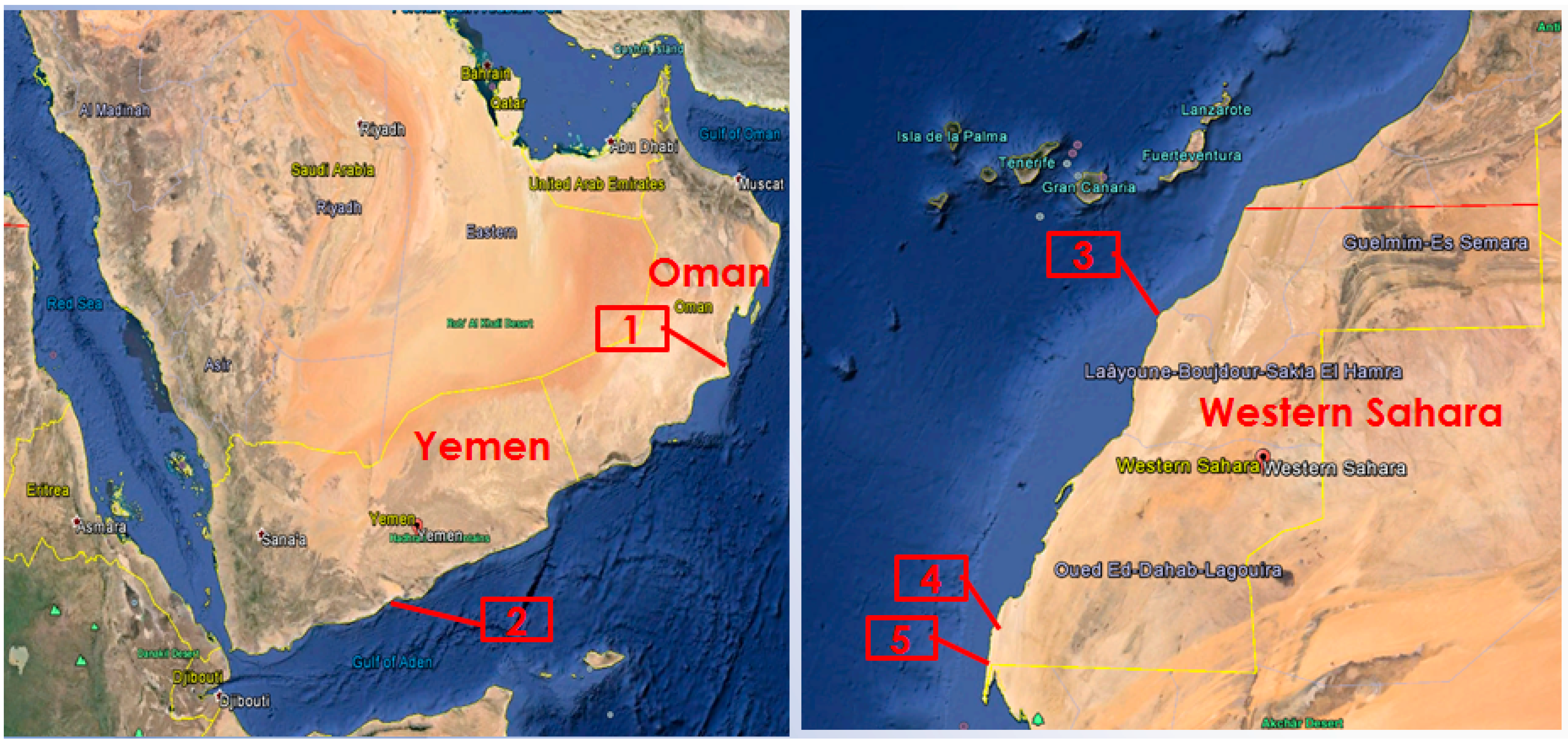
3.2.1. Site Selection


| Site | Number of Scenes | Start Date | End Date |
|---|---|---|---|
| Oman | 12 | 15 April 2013 | 4 May 2014 |
| Yemen | 5 | 27 October 2013 | 21 April 2014 |
| Western Sahara 1 | 8 | 11 June 2013 | 30 June 2014 |
| Western Sahara 2 | 12 | 1 May 2013 | 18 April 2014 |
| Western Sahara 3 | 12 | 1 May 2013 | 18 April 2014 |
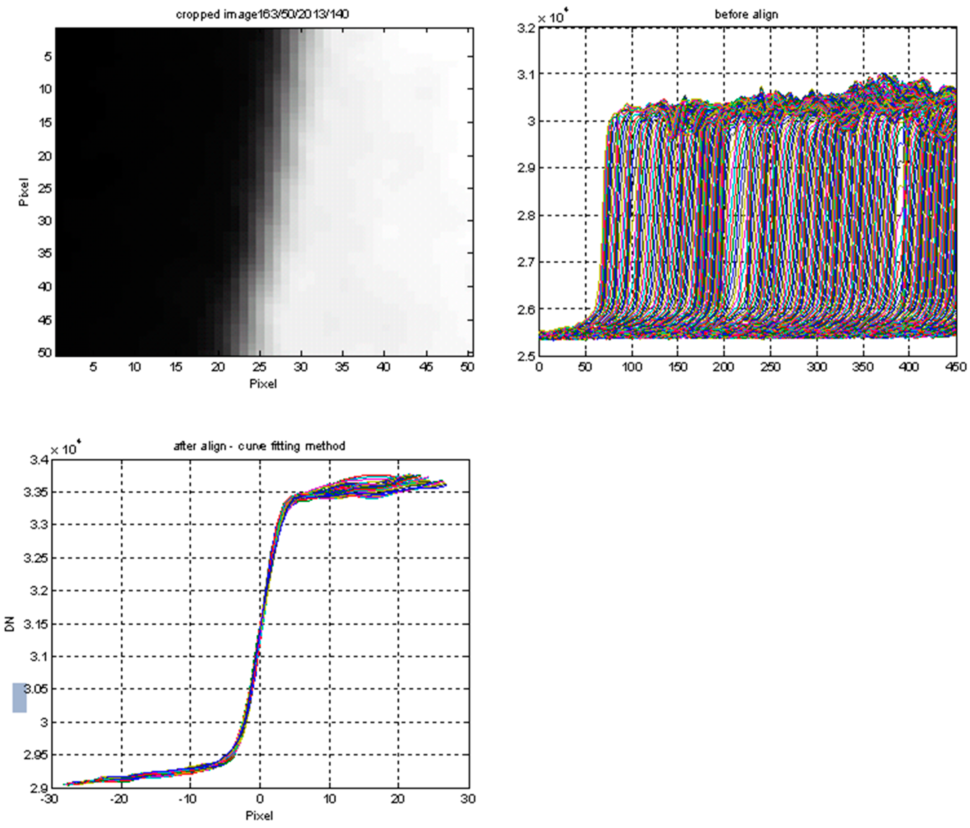
3.2.2. Processing Steps

4. Results and Discussion
4.1. Pre-Launch
| SCA | Column | Row | Edge Slope | Edge Extent (m) | ||
|---|---|---|---|---|---|---|
| Cross-Track | Along-Track | Cross-Track | Along-Track | |||
| A | 602.96 | 5.65 | 0.53 | 0.46 | 230.16 | 271.80 |
| A | 262.15 | 6.33 | 0.60 | 0.51 | 198.10 | 247.40 |
| A | 23.13 | 9.91 | 0.60 | 0.52 | 200.38 | 240.34 |
| A | 19.05 | 8.40 | 0.60 | 0.54 | 197.09 | 235.02 |
| C | 21.64 | 12.01 | 0.60 | 0.56 | 199.97 | 216.49 |
| C | 24.02 | 11.35 | 0.60 | 0.55 | 201.45 | 221.29 |
| C | 315.32 | 9.28 | 0.60 | 0.55 | 195.85 | 214.96 |
| C | 601.52 | 12.36 | 0.59 | 0.56 | 204.69 | 217.83 |
| C | 602.57 | 9.55 | 0.59 | 0.55 | 204.34 | 222.73 |
| B | 601.13 | 1.03 | 0.59 | 0.53 | 198.18 | 224.76 |
| B | 599.97 | 3.48 | 0.60 | 0.52 | 197.82 | 257.29 |
| B | 263.40 | 9.82 | 0.60 | 0.51 | 197.91 | 237.75 |
| B | 23.29 | 10.38 | 0.57 | 0.48 | 210.00 | 234.55 |
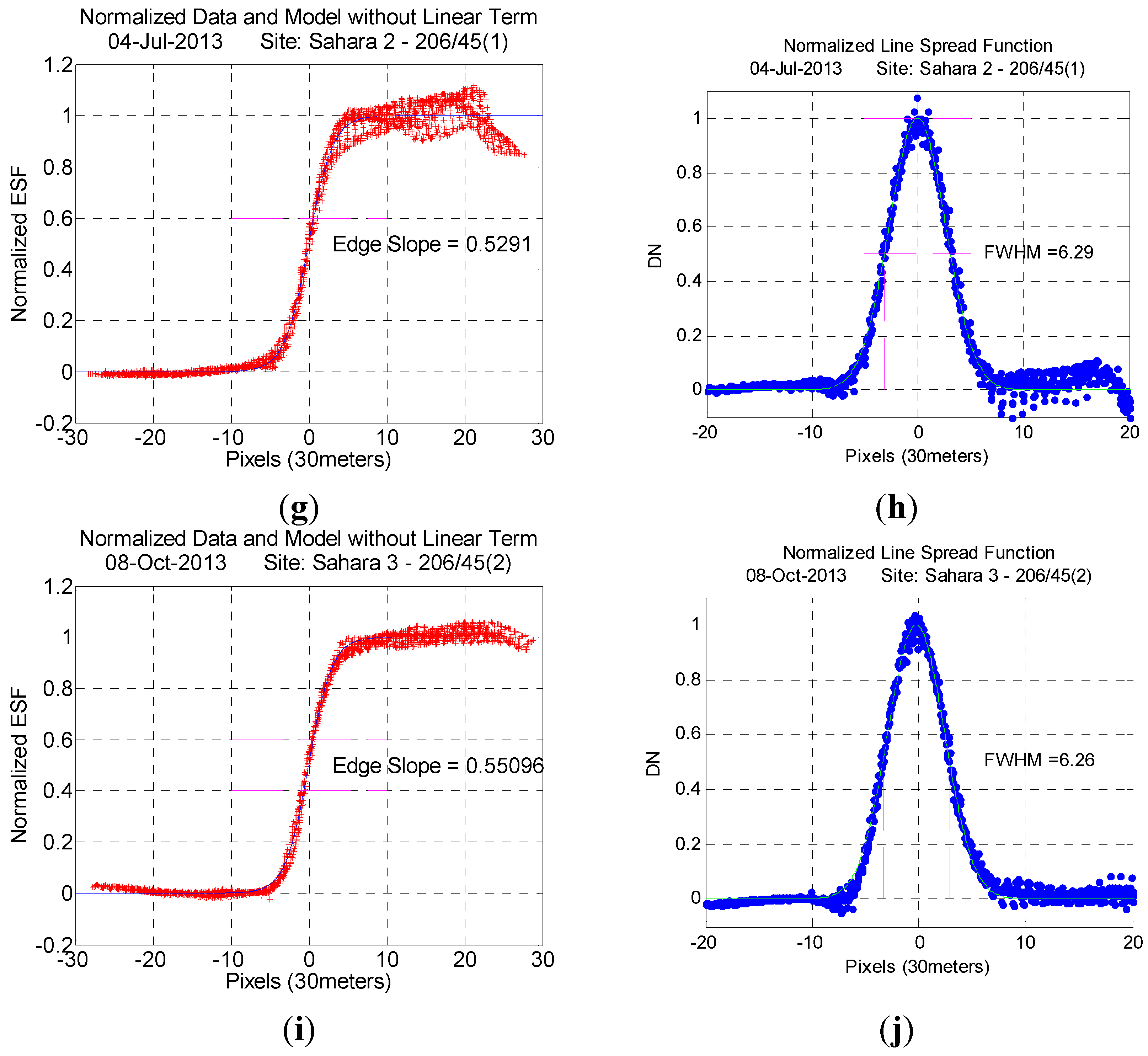
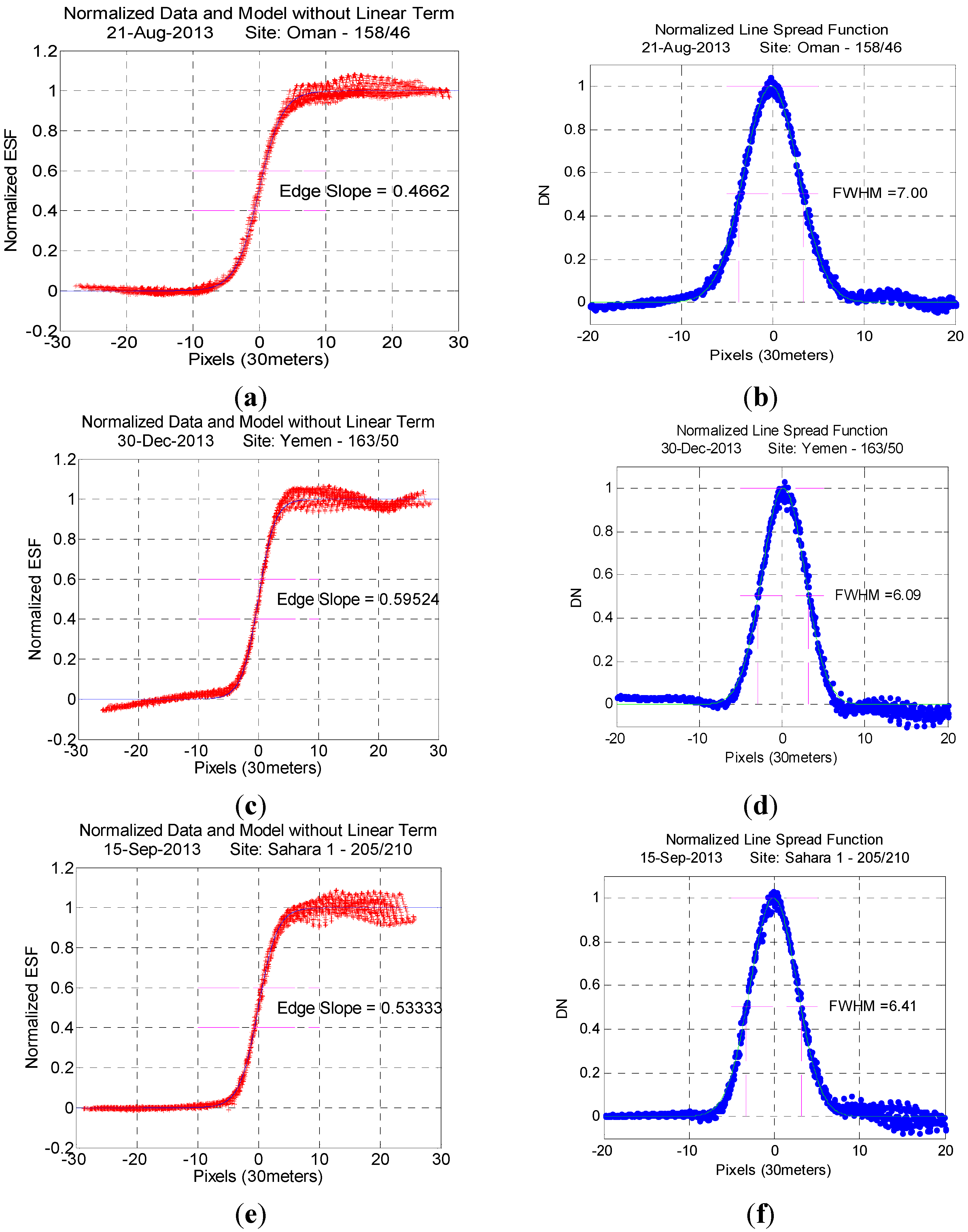
4.2. Post-Launch
| Sites | Rotation | Path/Row | SNR | Edge Slope | SD | FWHM (30 m Pixel) | SD | FWHM (Meters) | SD |
|---|---|---|---|---|---|---|---|---|---|
| Oman | 180° | 158/46 | 43 | 0.469 | 0.027 | 7.07 | 0.25 | 212.1 | 7.5 |
| Yemen | 90° | 163/50 | 57 | 0.577 | 0.029 | 6.11 | 0.07 | 183.3 | 2.1 |
| Western Sahara 1 | 0° | 205/42 | 37 | 0.528 | 0.030 | 6.41 | 0.11 | 192.6 | 3.3 |
| Western Sahara 2 | 0° | 206/45 | 34 | 0.537 | 0.031 | 6.22 | 0.18 | 186.9 | 3.0 |
| Western Sahara 3 | 0° | 206/45 | 54 | 0.545 | 0.014 | 6.37 | 0.13 | 191.1 | 3.9 |
5. Conclusions
Acknowledgments
Author Contributions
Conflicts of Interest
References
- Williams, D.L.; Goward, S.N.; Arvidson, T.J. Landsat: Yesterday, today, and tomorrow. Photogram. Eng. Remote Sens. 2006, 72, 1171–1178. [Google Scholar] [CrossRef]
- Reuter, D.C.; Richardson, C.M.; Pellerano, F.A.; Irons, J.R.; Allen, R.G.; Anderson, M.; Jhabvala, M.D.; Lunsford, A.W.; Montanaro, M.; Smith, R.L.; et al. The Thermal Infrared Sensor (TIRS) on Landsat 8: Design overview and pre-launch characterization. Remote Sens. 2015, 7, 1135–1153. [Google Scholar] [CrossRef]
- Jhabvala, M.; Reuter, D.; Choi, K.; Jhabvala, C.; Sundaram, C. QWIP-based thermal infrared sensor for the Landsat Data Continuity Mission. Infrared Phys. Technol. 2009, 52, 424–429. [Google Scholar] [CrossRef]
- Thome, K.; Markham, B.; Barker, J.; Slater, P.; Biggar, S. Radiometric calibration of Landsat. Photogram. Eng. Remote Sens. 1997, 63, 853–858. [Google Scholar]
- Montanaro, M.; Levy, R.; Markham, B. On-Orbit radiometric performance of the Landsat 8 thermal infrared sensor. Remote Sens. 2014, 6, 11753–11769. [Google Scholar] [CrossRef]
- Holst, G.C. Electro-Optical Imaging System Performance; The International Society for Optical Engineering: Bellingham, DC, USA, 1995. [Google Scholar]
- Schowengerdt, R.A.; Archwamety, C.; Wrigley, R.C. Landsat thematic mapper image-derived MTF. Photogram. Eng. Remote Sens. 1985, 51, 1395–1406. [Google Scholar]
- Pagnutti, M.; Blonski, S.; Cramer, M.; Helder, D.; Holekamp, K.; Honkavaara, E.; Ryan, R. Targets, methods, and sites for assessing the in-flight spatial resolution of electro-optical data products. Can. J. Remote Sens. 2010, 36, 583–601. [Google Scholar] [CrossRef]
- Braga, A.B.; Schowengerdt, R.A.; Rojas, F.; Biggar, S. Calibration of the MODIS PFM SRCA for on-orbit cross-track MTF measurement. Proc. SPIE 2000. [Google Scholar] [CrossRef]
- Oh, E.; Cho, S.; Ahn, Y-H.; Park, Y.; Ryu, J-H.; Kim, S-W. In-orbit optical performance assessment of geostationary ocean color imager. In Proceedings of the 2012 IEEE International Geoscience and Remote Sensing Symposium (IGARSS), Munich, Germany, 22–27 July 2012.
- Helder, D.; Choi, T.; Rangaswamy, M. In-flight characterization of spatial quality using point spread functions. In Proceedings of the 2004 International Workshop on Radiometric and Geometric Calibration, Gulfport, MI, USA, 2–5 December 2004.
- Choi, T. IKONOS Satellite on Orbit Modulation Transfer Function (MTF) Measurement Using Edge and Pulse Method. Master Thesis, South Dakota State University, Brookings, SD, USA, 2002. [Google Scholar]
- Leger, D.; Duffaut, J.; Robinet, F. MTF measurements using spotlight. In Proceedings of the 1994 International Geoscience And Remote Sensing Symposium, Pasadena, CA, USA, 8–12 August 1994.
- Bowen, H.S.; Dial, G. IKONOS calculation of MTF using stellar images. In Proceedings of the 2002 High Spatial Resolution Commercial Imagery Workshop, Reston, VA, USA, 25–27 March 2002.
- Storey, J. Landsat 7 on-orbit modulation transfer function estimation. Proc. SPIE 2001. [Google Scholar] [CrossRef]
- Thome, K.; Reuter, D.; Lunsford, A.; Montanaro, M.; Wenny, B.N.; Tesfaye, Z. Calibration plan for the thermal infrared sensor on the Landsat data continuity mission. In Proceedings of the 2010 CALCON Technical Conference, Logan, UT, USA, 23–26 August 2010.
- Savitzky, A.; Golay, M. Smoothing and differentiation of data by simplified least squares procedures. Anal. Chem. 1964, 36, 1627–1639. [Google Scholar] [CrossRef]
- Gerace, A.; College of Science, Rochester Institute of Technology. Personal communication. 2012. [Google Scholar]
- Helder, D.; Choi, J. On-orbit Modulation Transfer Function (MTF) measurement of QuickBird. In Proceedings of the 2003 High Spatial Resolution Commercial Imagery Workshop, Rseton, VA, USA, 19–21 May 2003.
© 2015 by the authors; licensee MDPI, Basel, Switzerland. This article is an open access article distributed under the terms and conditions of the Creative Commons Attribution license (http://creativecommons.org/licenses/by/4.0/).
Share and Cite
Wenny, B.N.; Helder, D.; Hong, J.; Leigh, L.; Thome, K.J.; Reuter, D. Pre- and Post-Launch Spatial Quality of the Landsat 8 Thermal Infrared Sensor. Remote Sens. 2015, 7, 1962-1980. https://doi.org/10.3390/rs70201962
Wenny BN, Helder D, Hong J, Leigh L, Thome KJ, Reuter D. Pre- and Post-Launch Spatial Quality of the Landsat 8 Thermal Infrared Sensor. Remote Sensing. 2015; 7(2):1962-1980. https://doi.org/10.3390/rs70201962
Chicago/Turabian StyleWenny, Brian N., Dennis Helder, Jungseok Hong, Larry Leigh, Kurtis J. Thome, and Dennis Reuter. 2015. "Pre- and Post-Launch Spatial Quality of the Landsat 8 Thermal Infrared Sensor" Remote Sensing 7, no. 2: 1962-1980. https://doi.org/10.3390/rs70201962
APA StyleWenny, B. N., Helder, D., Hong, J., Leigh, L., Thome, K. J., & Reuter, D. (2015). Pre- and Post-Launch Spatial Quality of the Landsat 8 Thermal Infrared Sensor. Remote Sensing, 7(2), 1962-1980. https://doi.org/10.3390/rs70201962