
An Improved Unmixing-Based Fusion Method: Potential Application to Remote Monitoring of Inland Waters

Abstract
:1. Introduction
2. Materials
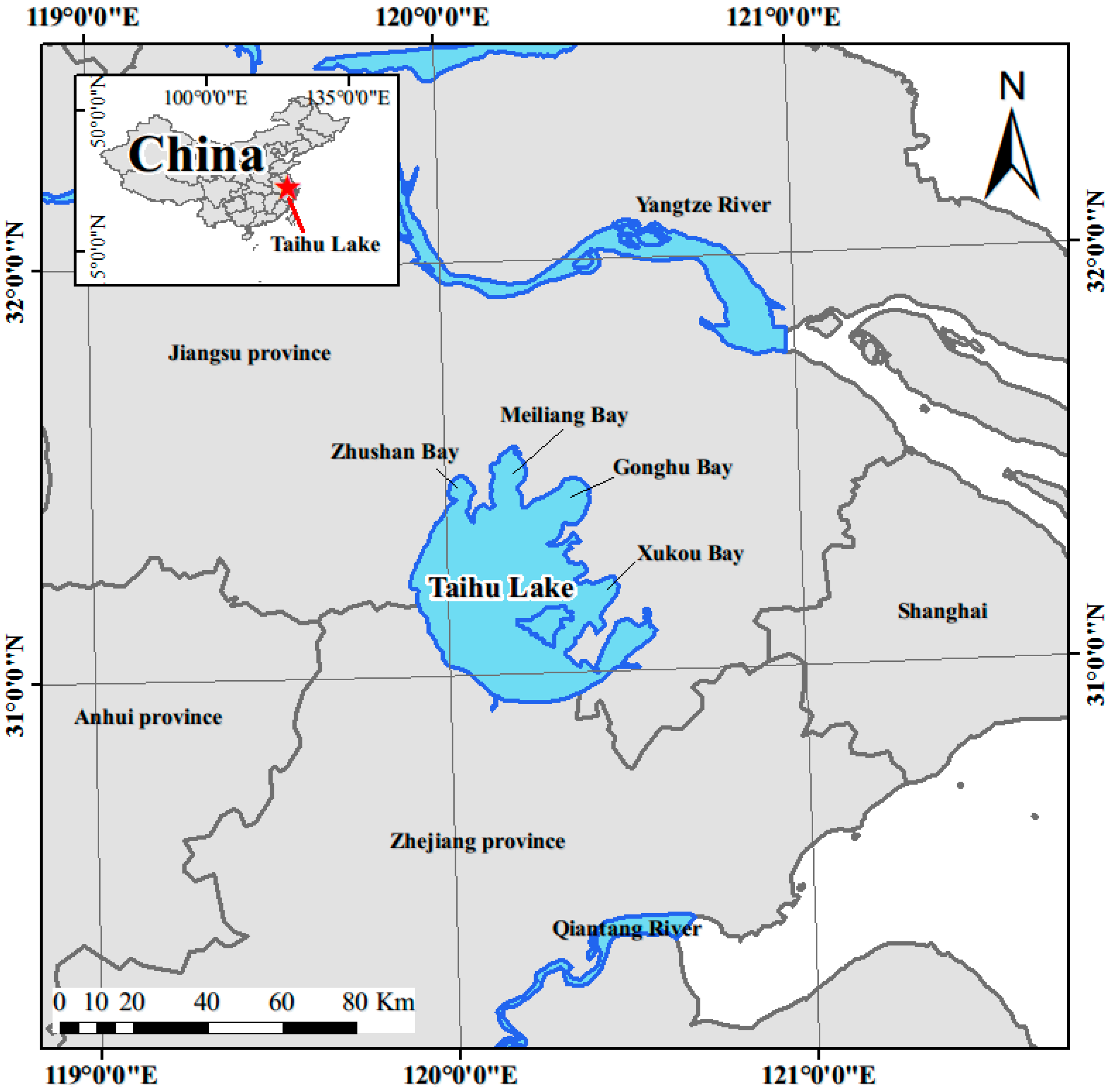
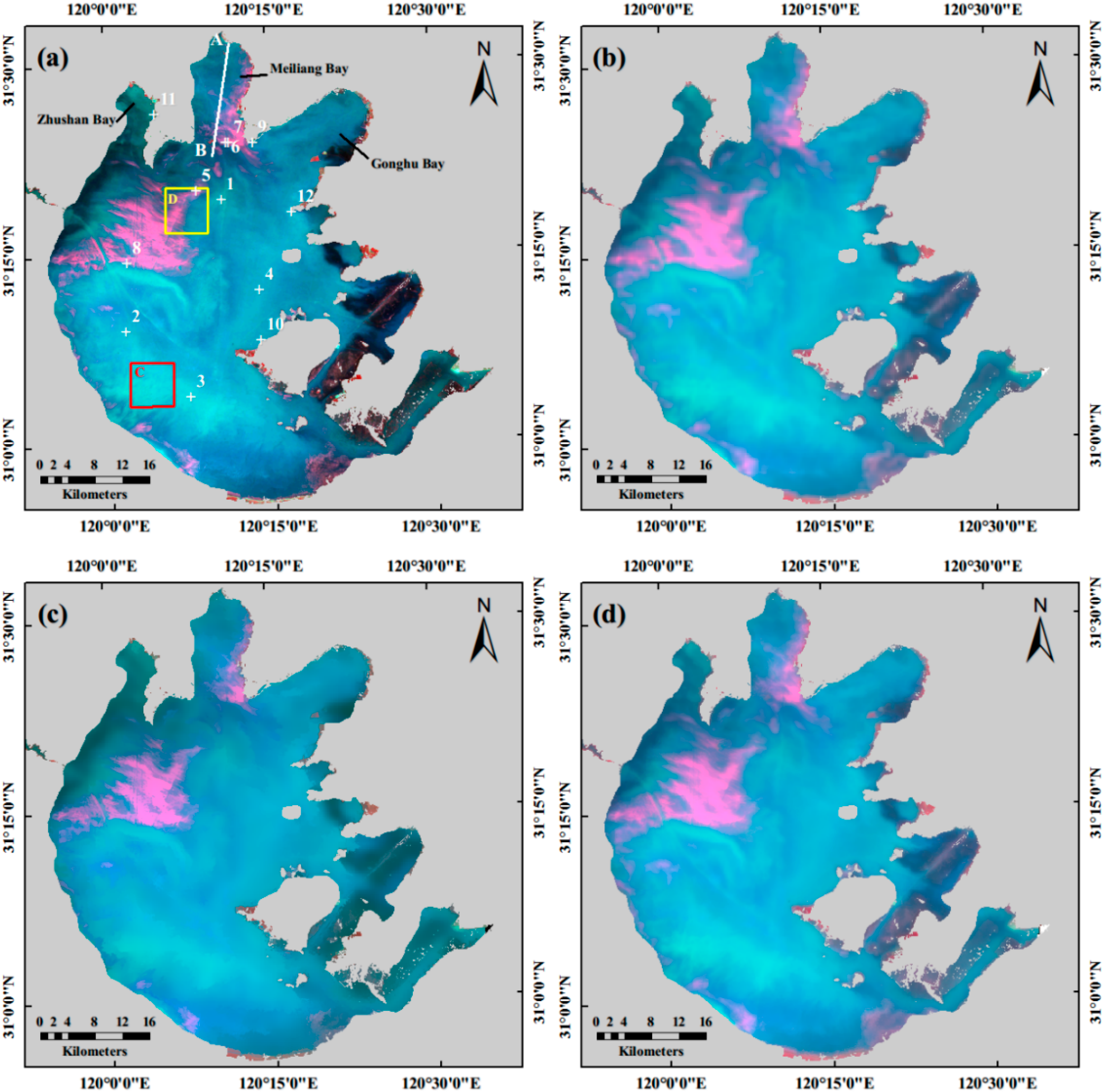
2.1. Study Area
2.2. Datasets

| Dataset | Date | Image Data | Sensing Time Difference | Usage |
|---|---|---|---|---|
| #1 | 5 October 2010 | HJ1-CCD image; MERIS image | 6 min | Algorithm validation and parameter optimisation |
| #2 | 9 August 2010 | HJ1-CCD image; MERIS image; | 7 min | Algorithm application |
| Specifications | HJ1-CCD | MERIS | ||
|---|---|---|---|---|
| Swath width(km) | 360 | 1150 | ||
| Altitude(km) | 750 | 800 | ||
| Spatial resolution(m) | 30 | 1200/300 | ||
| Revisit time(days) | 2 | 3 | ||
| Quantitative value(bit) | 8 | 16 | ||
| Average Signal to noise ratio(dB) | ≥48 | 1650 | ||
| Band setting | Centre(nm) | Width(nm) | Centre(nm) | Width(nm) |
| 412.5 | 10 | |||
| 475 | 90 | 442.5 | 10 | |
| 490 | 10 | |||
| 510 | 10 | |||
| 560 | 80 | 560 | 10 | |
| 660 | 60 | 620 | 10 | |
| 665 | 10 | |||
| 681.25 | 7.5 | |||
| 708.75 | 10 | |||
| 753.75 | 7.5 | |||
| 830 | 140 | 761.875 | 3.75 | |
| 778.75 | 15 | |||
| 865 | 20 | |||
3. Methods
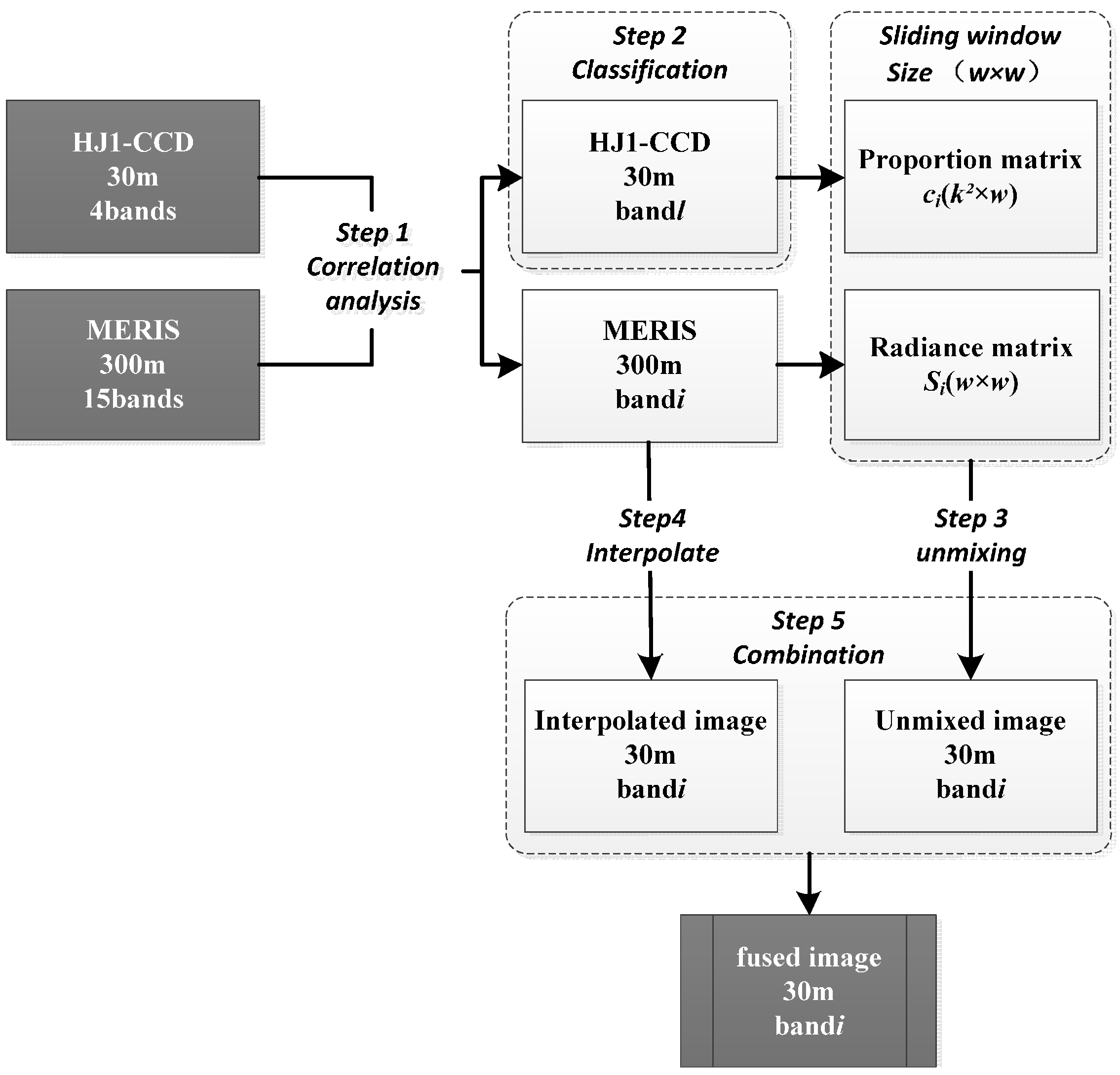
3.1. The Unmixing-Based Fusion (UBF) Method
3.2. Methodology Improvement

4. Results
4.1. Co-Registration Accuracy

4.2. Algorithm Validation
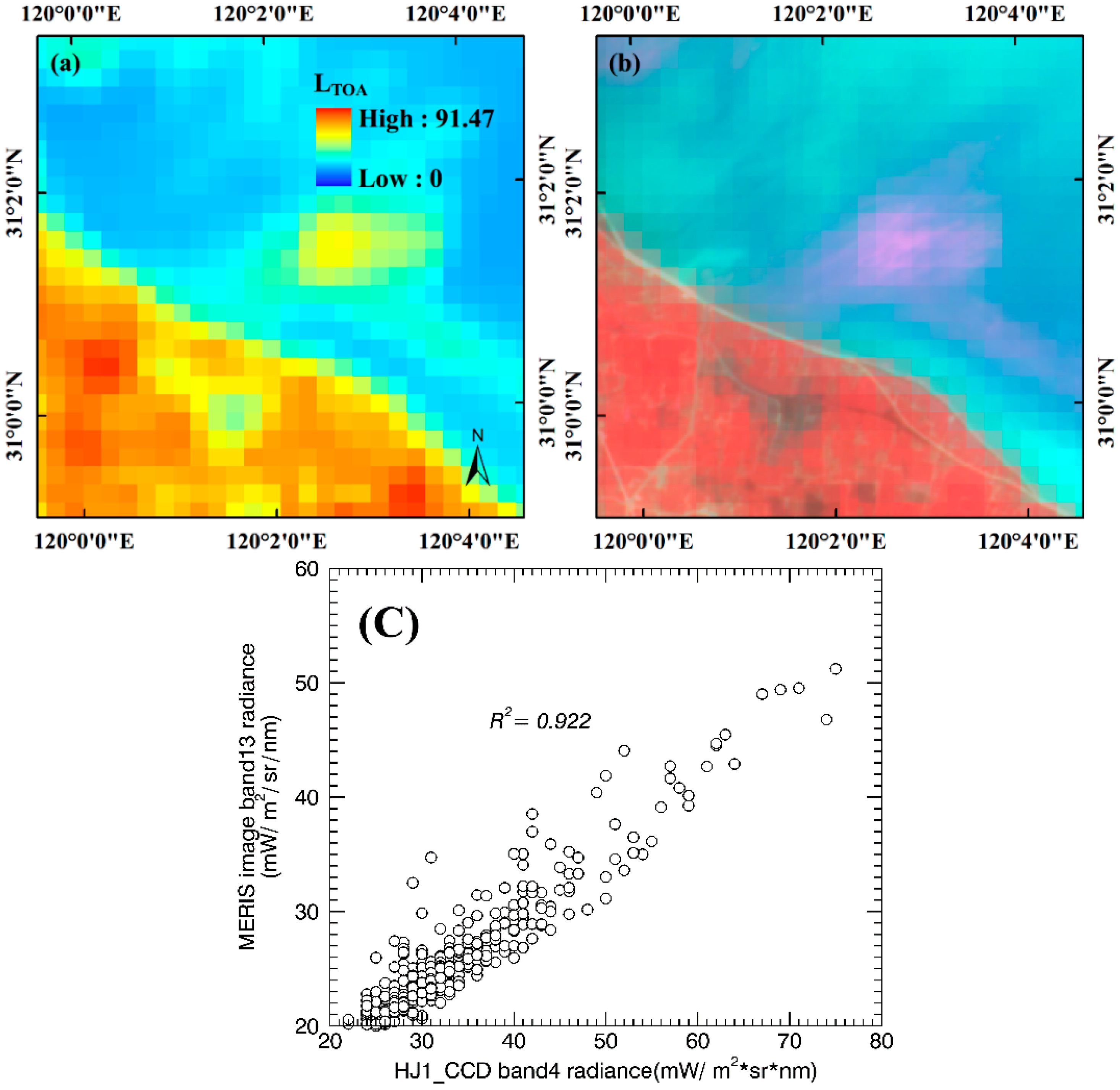
4.2.1. HJ1-CCD Band Selection
| MERIS Band | HJ1-CCD Band | R | MERIS Band | HJ1-CCD Band | R |
|---|---|---|---|---|---|
| 1 | 1 | 0.873 | 9 | 4 | 0.852 |
| 2 | 1 | 0.937 | 10 | 4 | 0.948 |
| 3 | 1 | 0.949 | 11 | 4 | 0.947 |
| 4 | 1 | 0.942 | 12 | 4 | 0.946 |
| 5 | 2 | 0.913 | 13 | 4 | 0.944 |
| 6 | 1 | 0.942 | 14 | 4 | 0.939 |
| 7 | 3 | 0.944 | 15 | 4 | 0.938 |
| 8 | 3 | 0.928 |
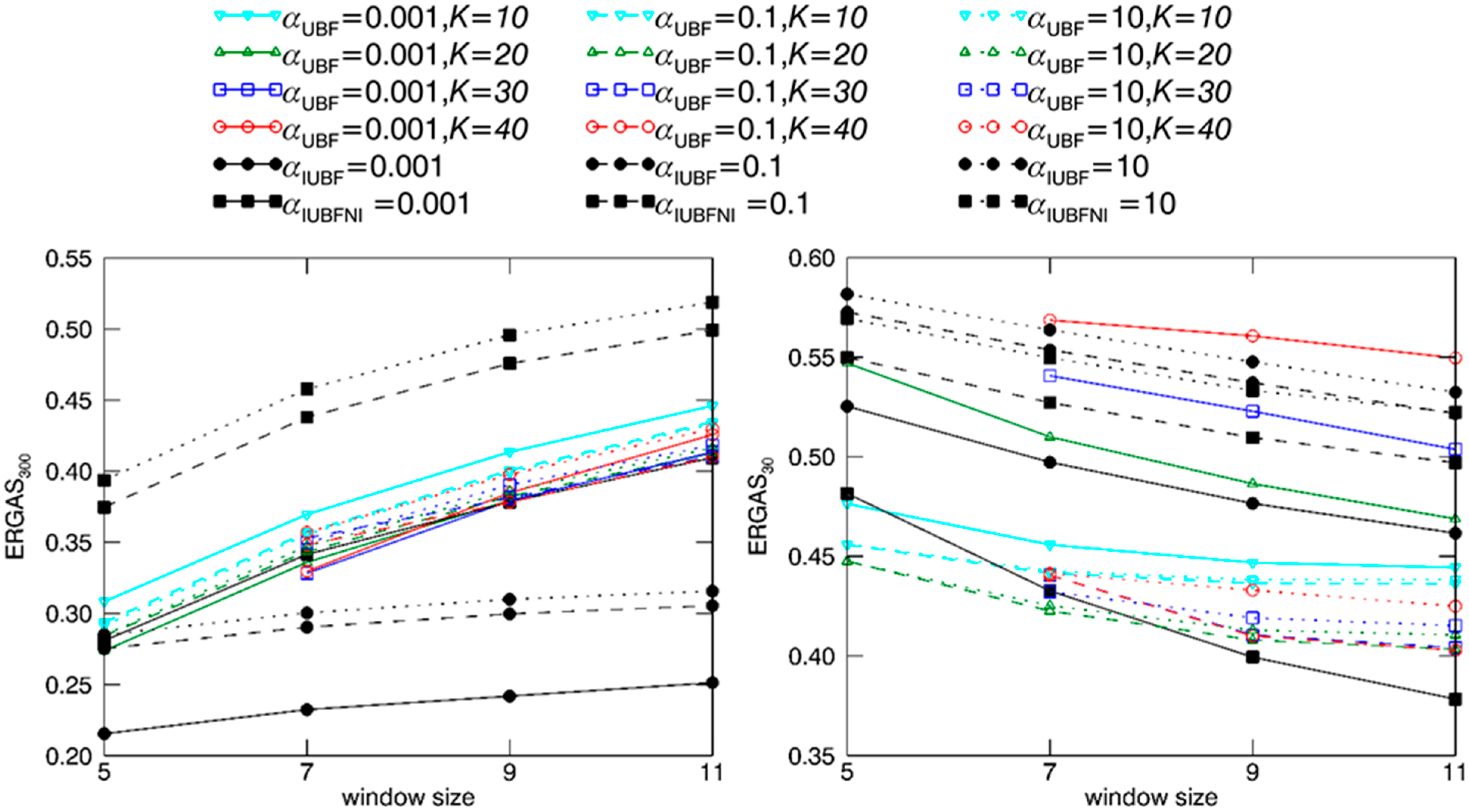
4.2.2. Free Parameter Optimisation

| w | α | K | ERGAS300 | ERGAS30 | |
|---|---|---|---|---|---|
| UBF | 7 | 0.1 | 40 | 0.348 | 0.440 |
| IUBF | 7 | 0.001 | - | 0.232 | 0.497 |
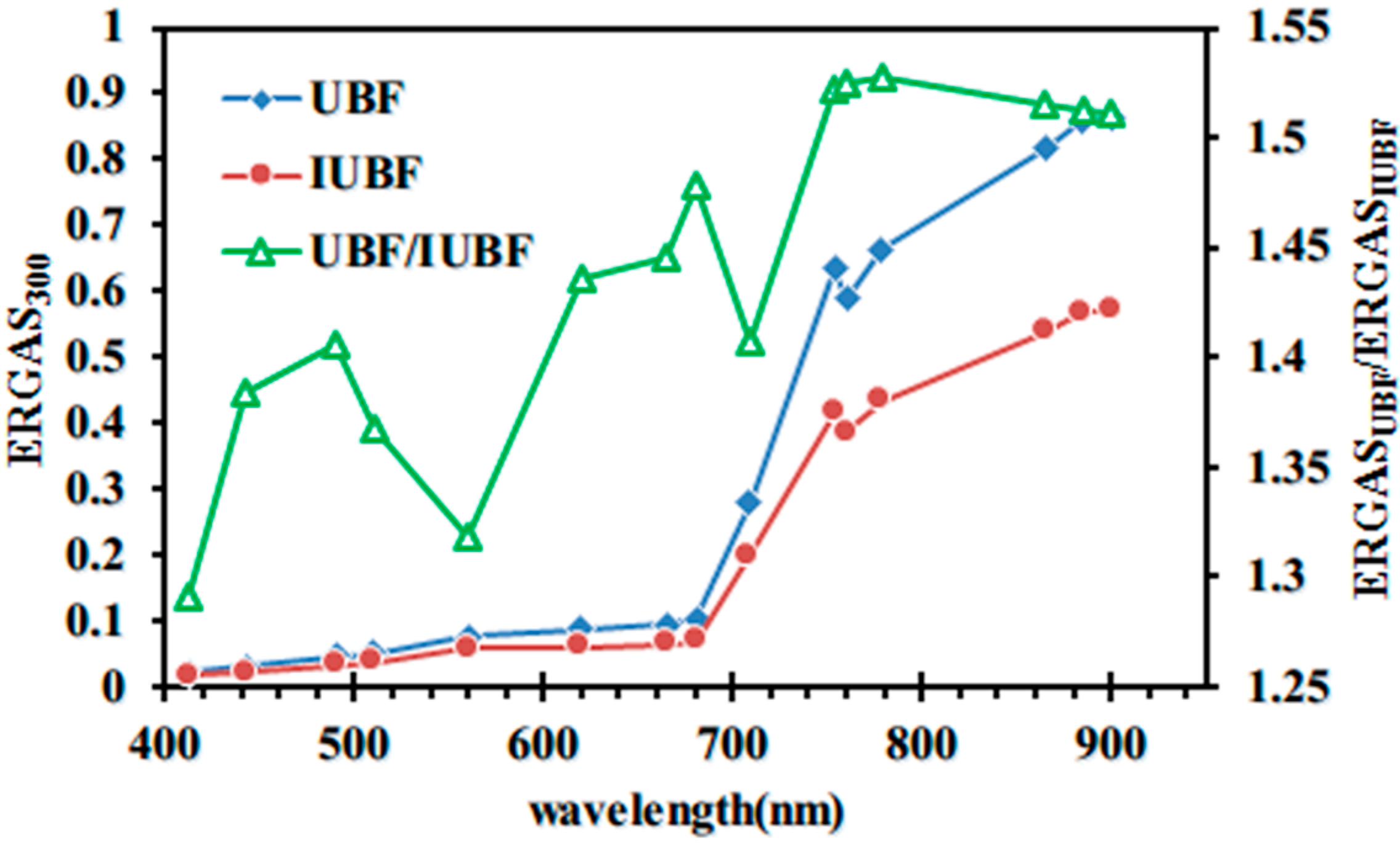
4.2.3. Interpolation Contribution
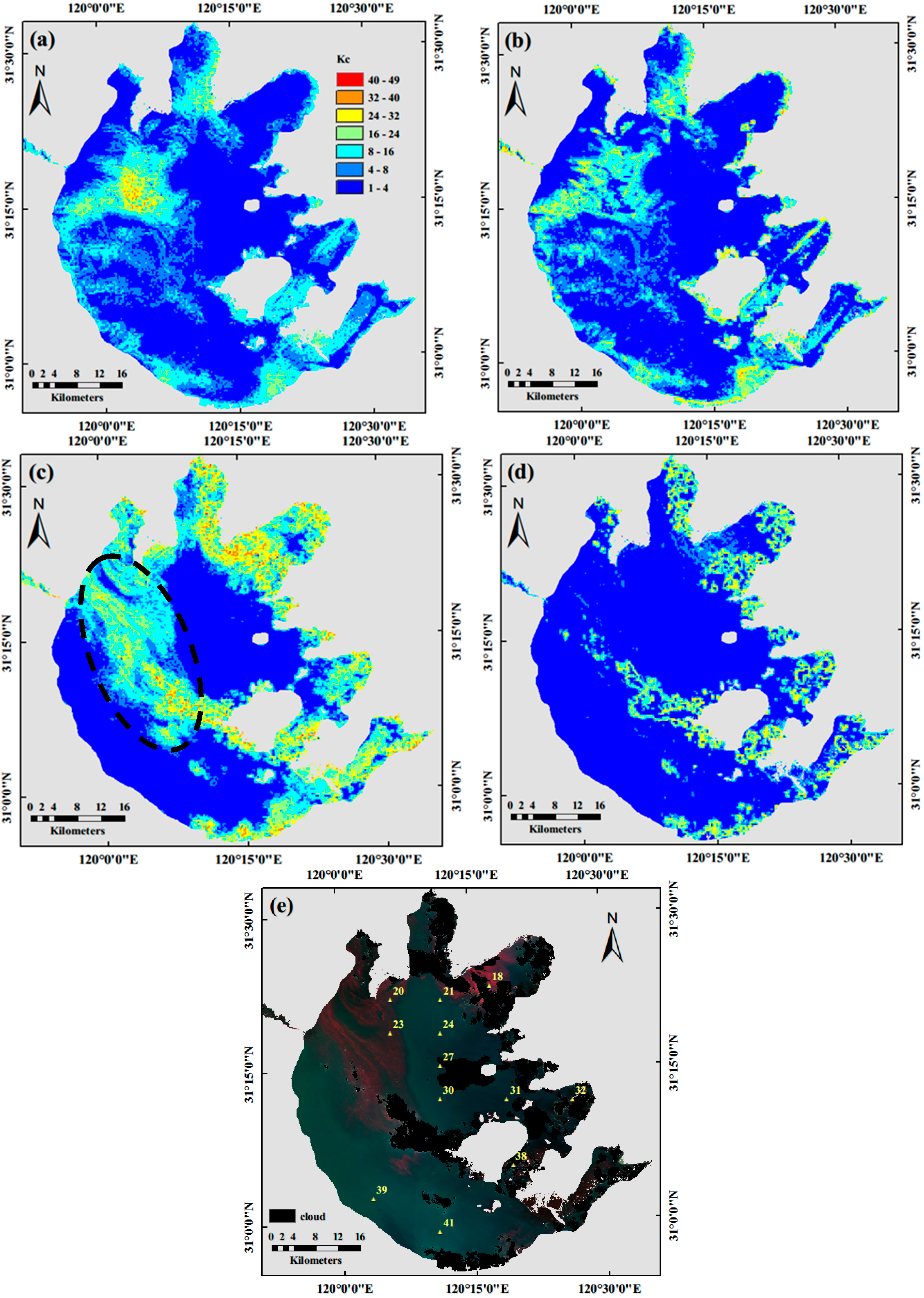
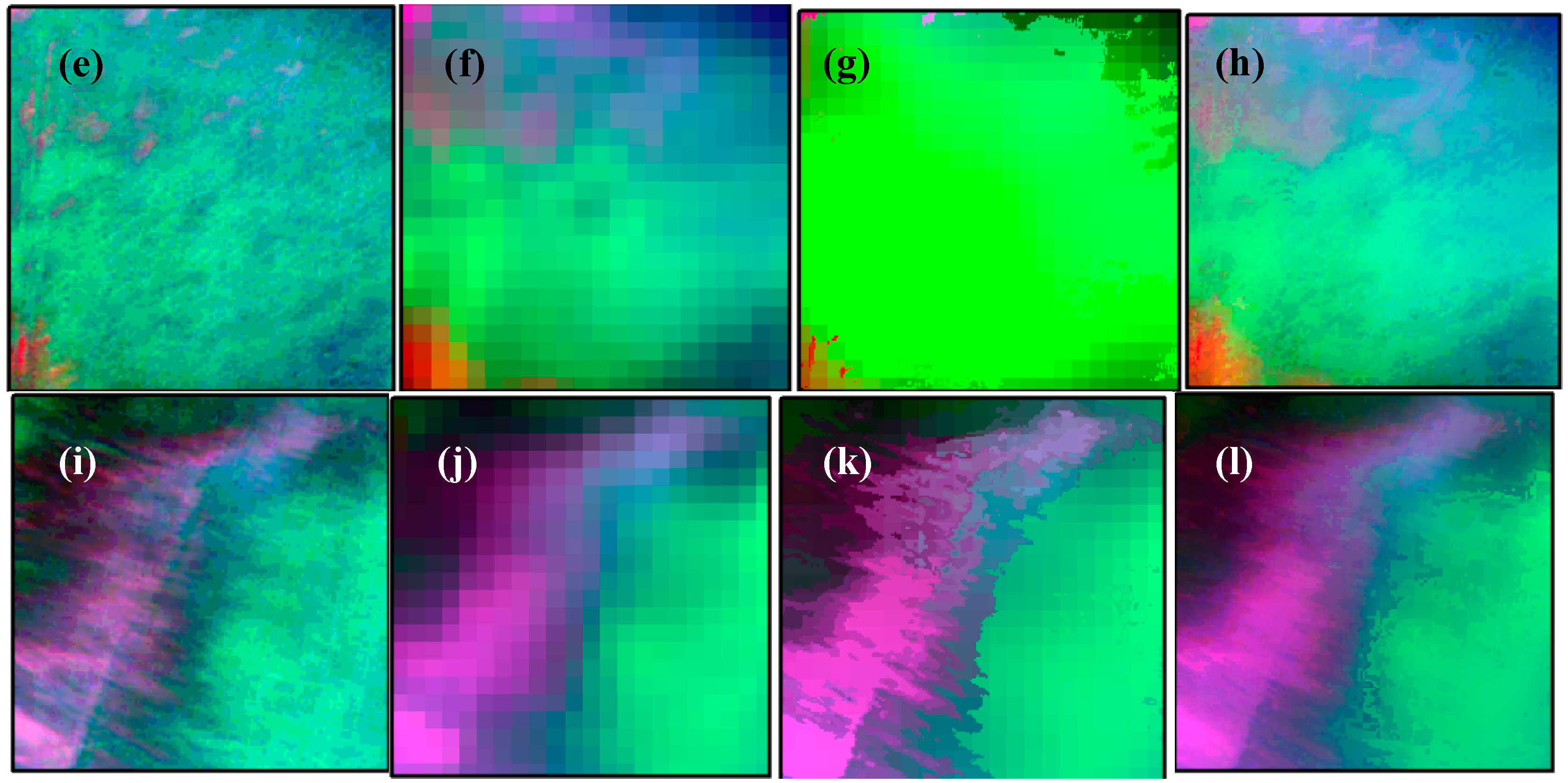
4.3. Evaluation of the Fusion Effect
4.3.1. Visual Effects

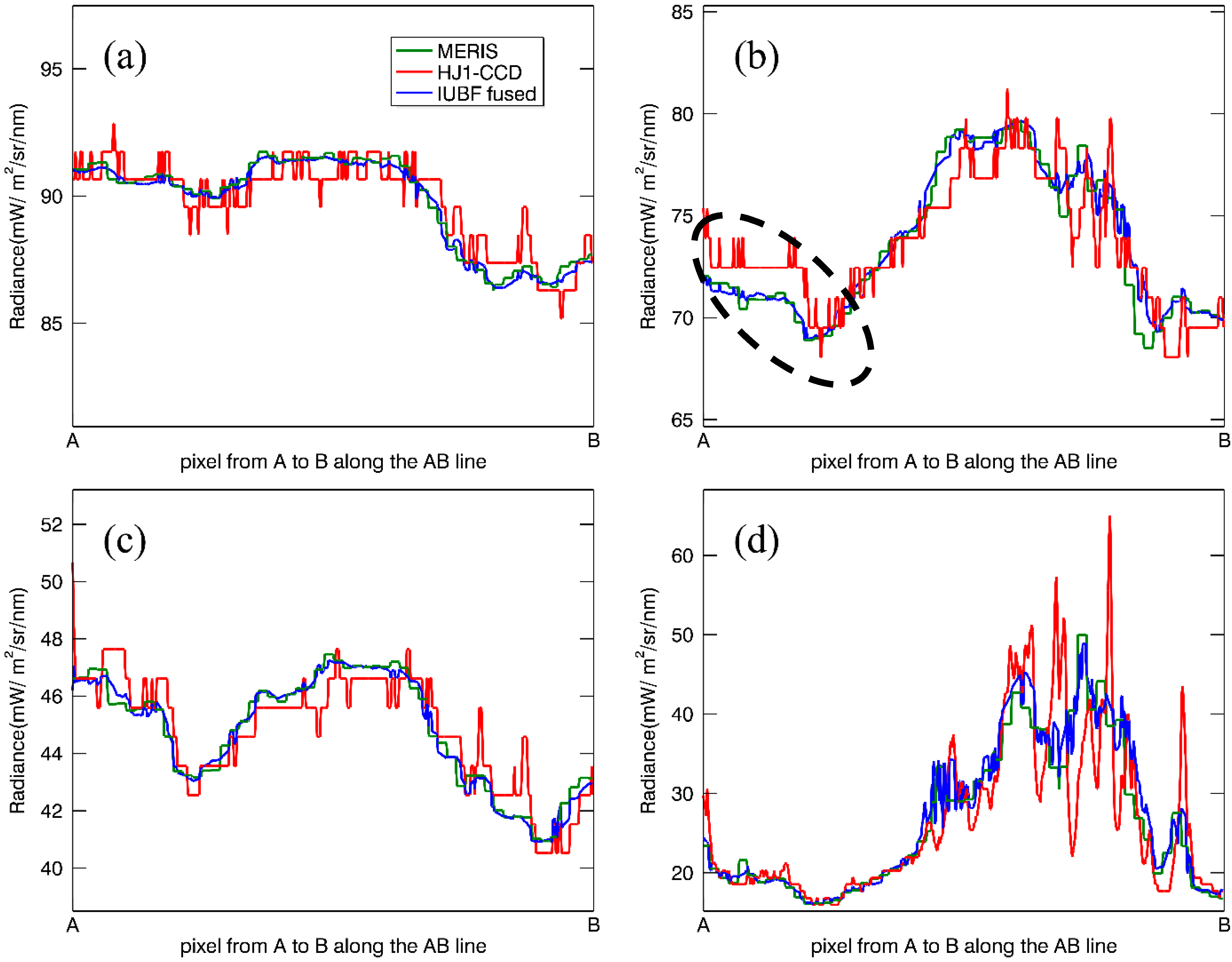
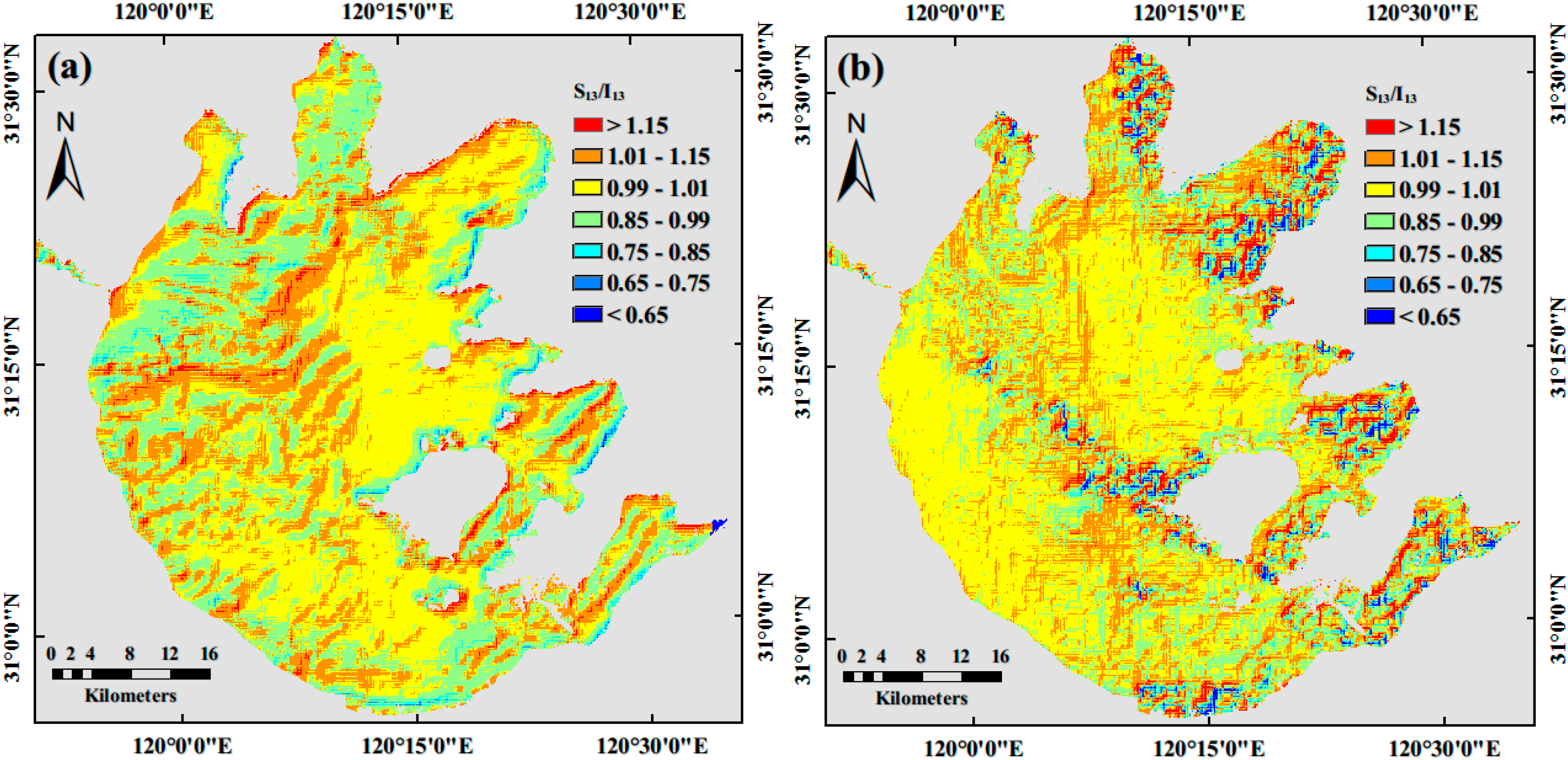
4.3.2. Radiance Changes

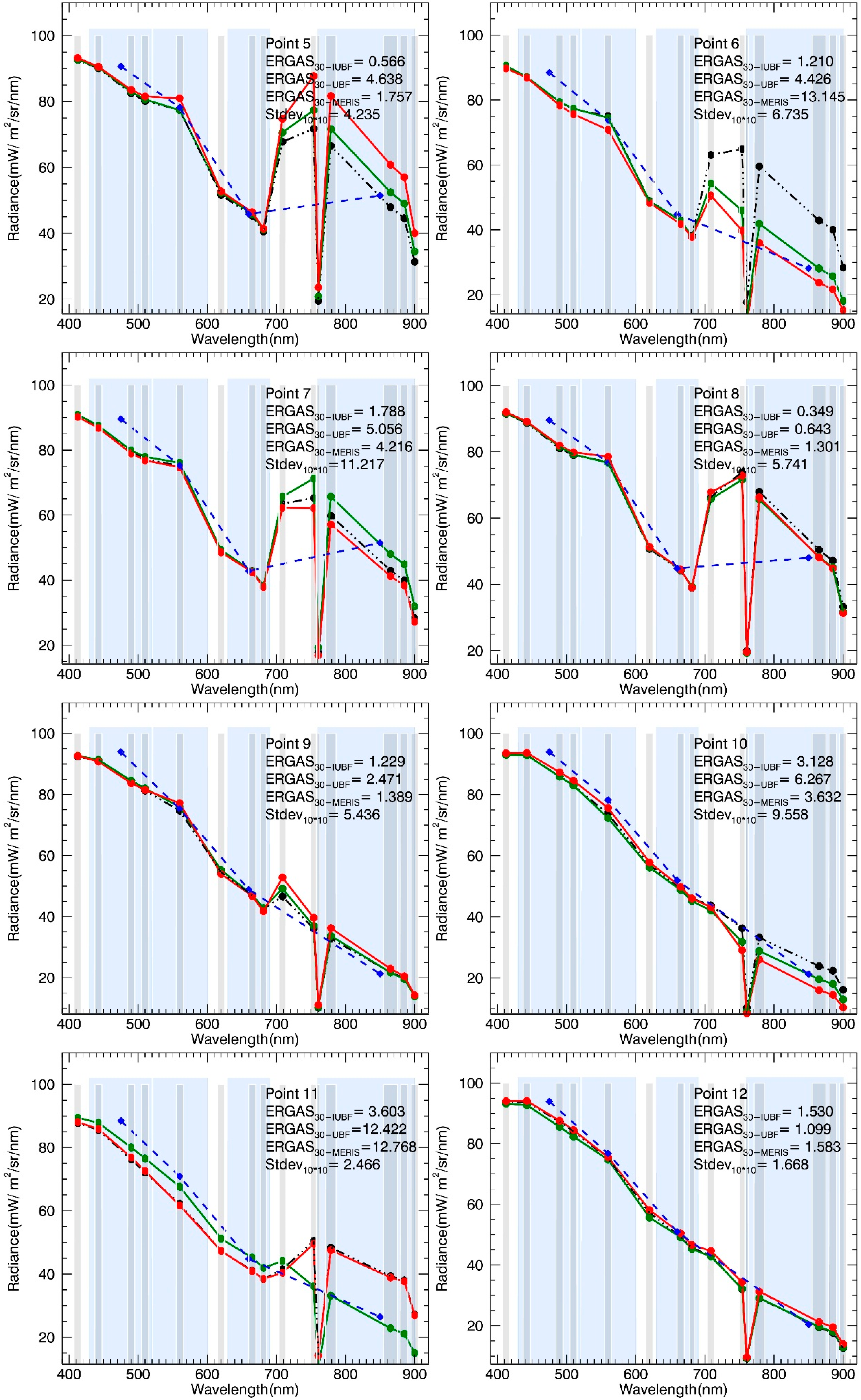
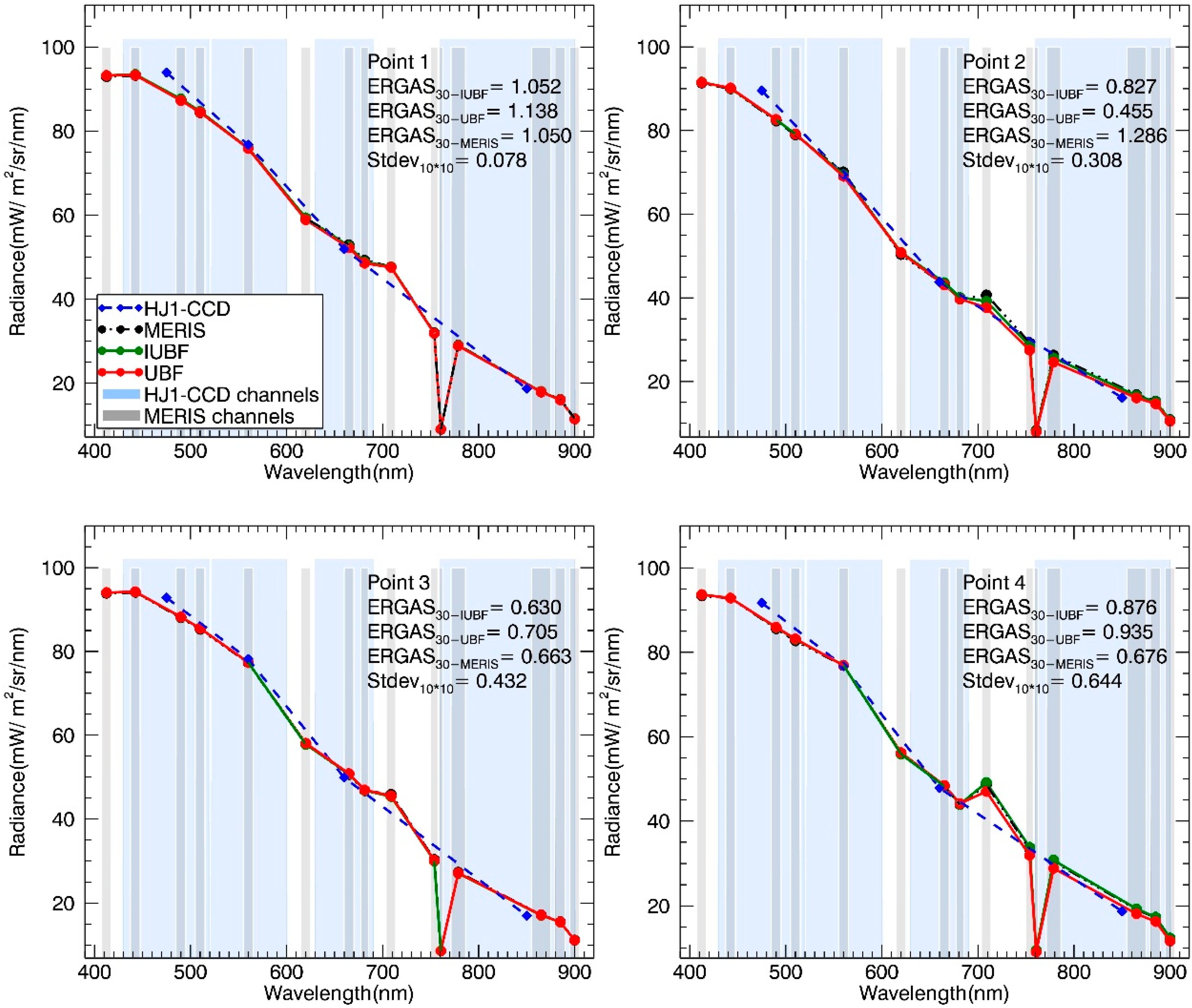
4.3.3. Spectrum Shape

5. Discussion
5.1. Robustness of the IUBF Algorithm
| w | α | K | ERGAS300 | ERGAS30 | |
|---|---|---|---|---|---|
| UBF | 7 | 0.1 | 40 | 0.447 | 1.301 |
| IUBF | 7 | 0.001 | - | 0.349 | 1.291 |


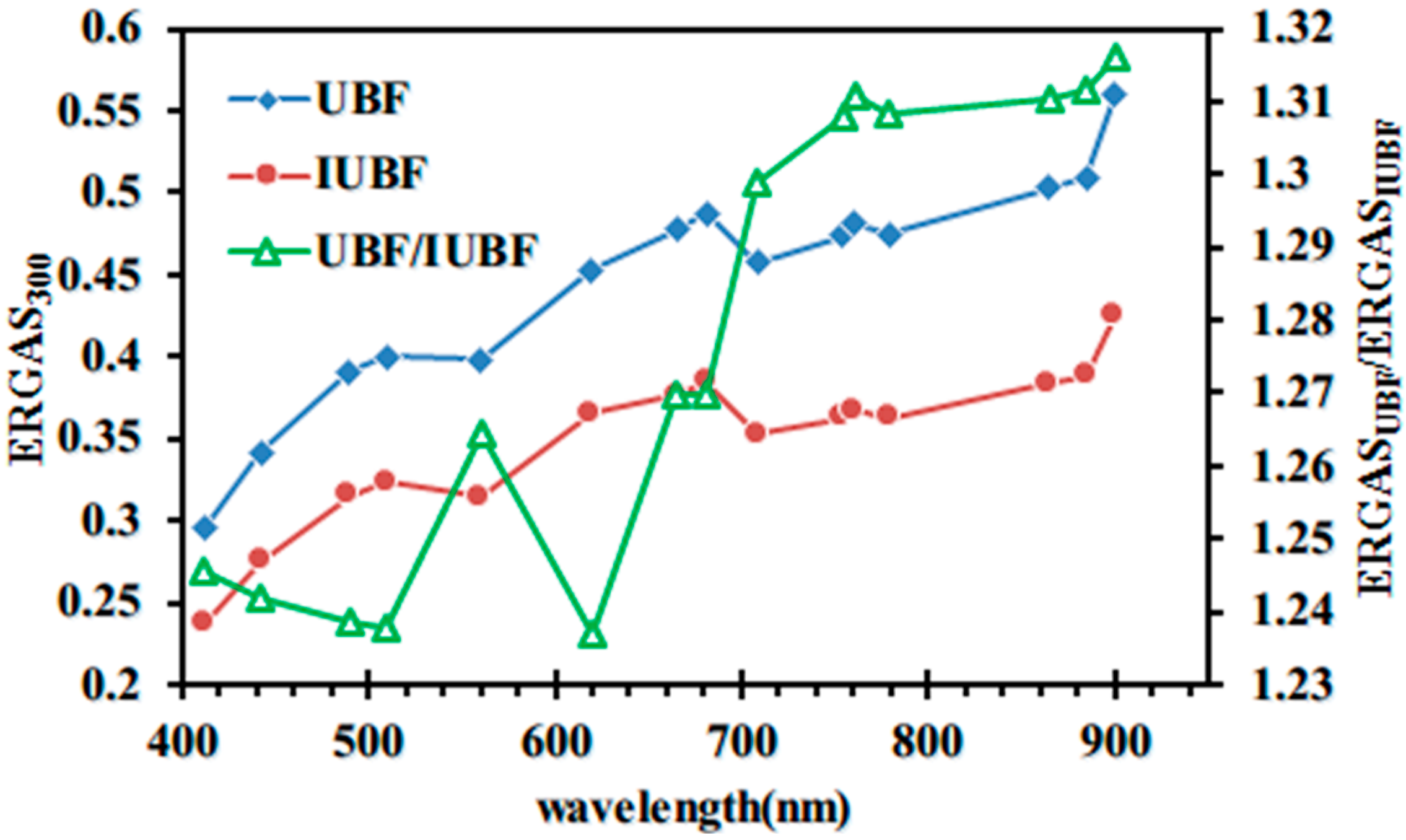
5.2. Interpolation Quality in the Spatial Scale

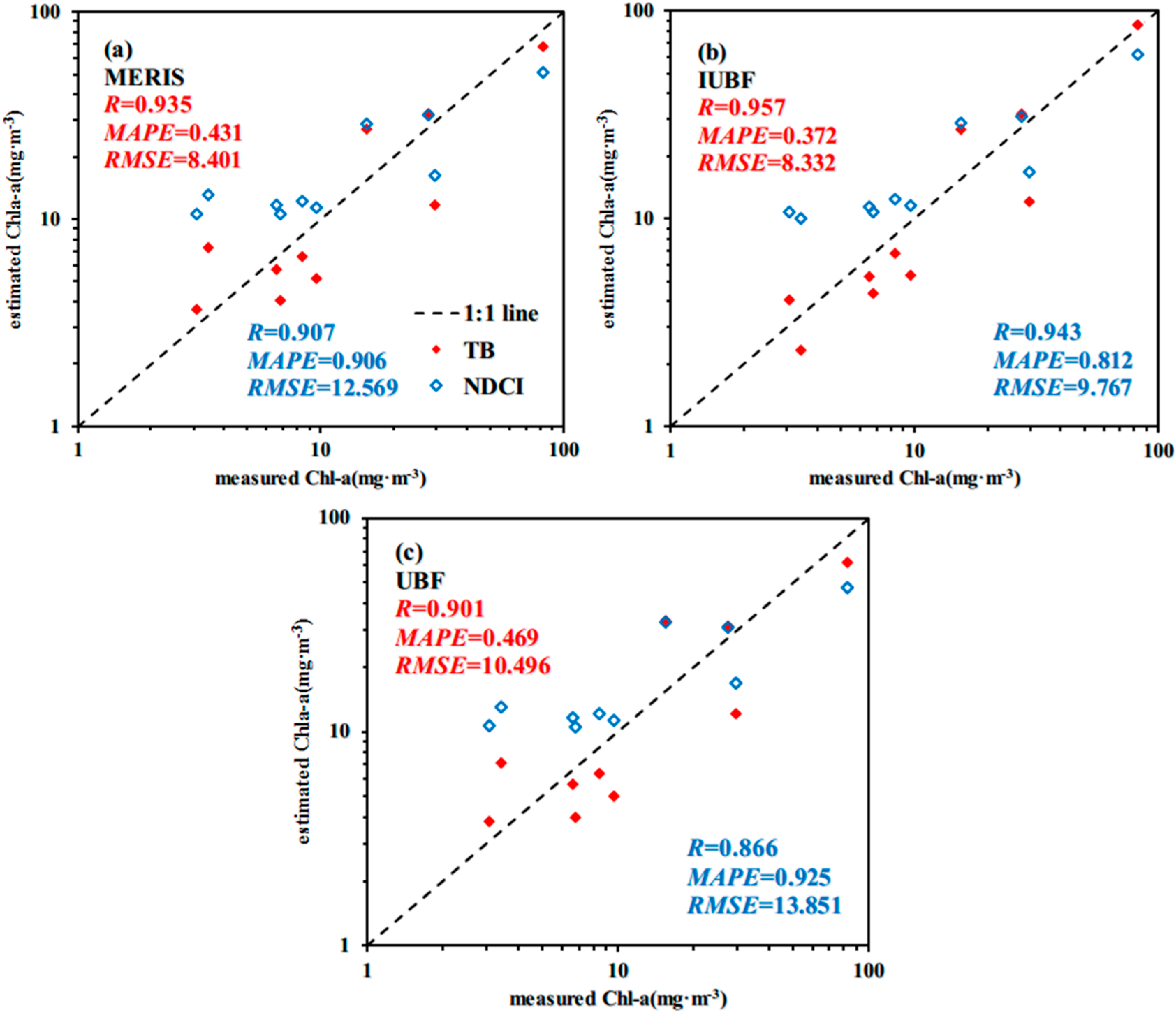
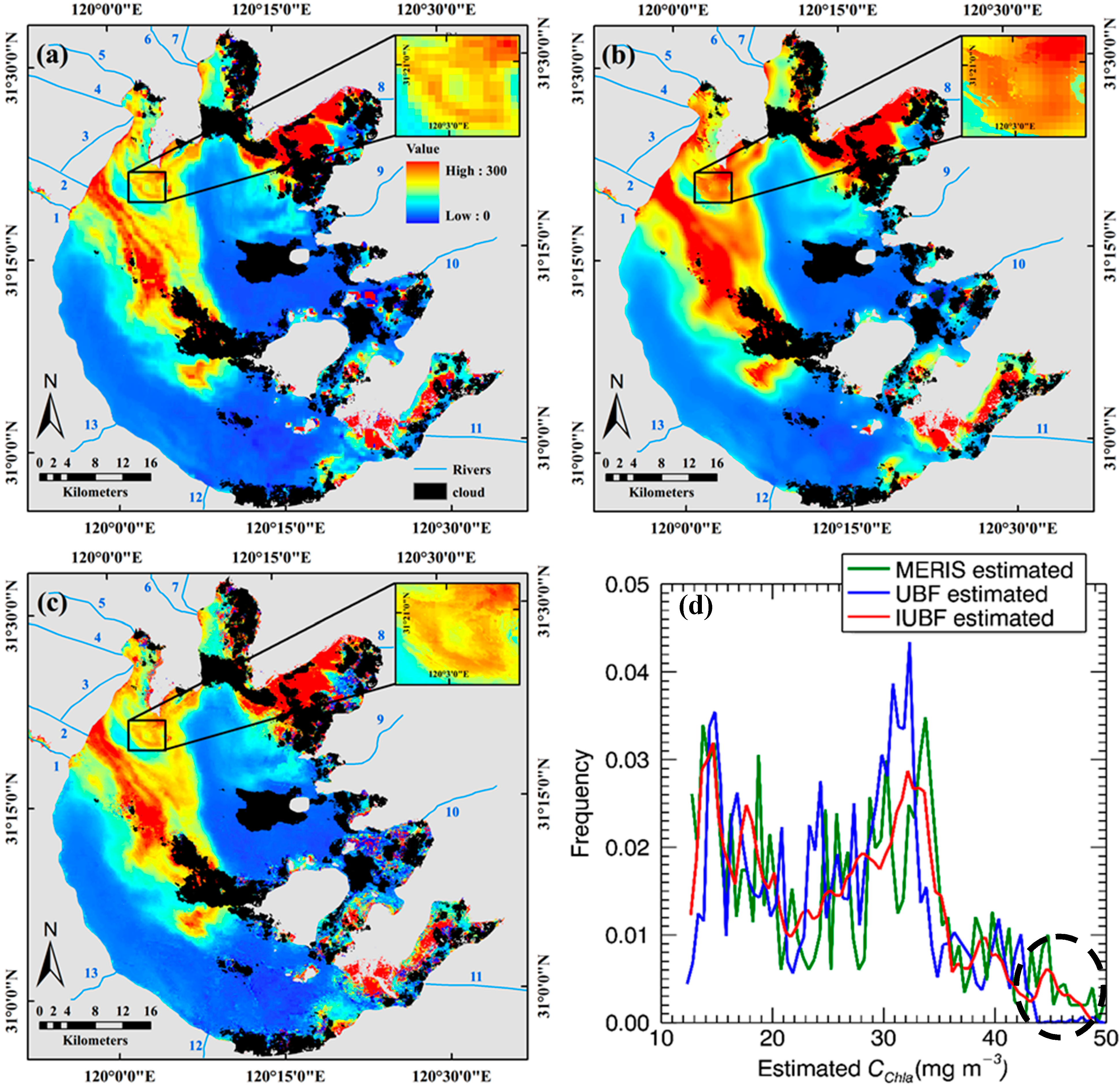
5.3. Potential Application of Remote Water Monitoring
6. Conclusions
Acknowledgments
Author Contributions
Conflicts of Interest
References
- Xiao, J.; Guo, Z. Detection of chlorophyll-a in urban water body by remote sensing. In Proceedings of the 2010 Second IITA International Conference on Geoscience and Remote Sensing (IITA-GRS), Qingdao, China, 28–31 August 2010; pp. 302–305.
- Li, Y.; Huang, J.; Lu, W.; Shi, J. Model-based remote sensing on the concentration of suspended sediments in Taihu Lake. Oceanol. Limnol. Sin. 2006, 37, 171–177, (in Chinese with English abstract). [Google Scholar]
- Li, Y.; Wang, Q.; Wu, C.; Zhao, S.; Xu, X.; Wang, Y.; Huang, C. Estimation of chlorophyll-a concentration using NIR/red bands of MERIS and classification procedure in inland turbid water. IEEE Trans. Geosci. Remote Sens. 2012, 50, 988–997. [Google Scholar] [CrossRef]
- Zhang, B.; Li, J.; Shen, Q.; Chen, D. A bio-optical model based method of estimating total suspended matter of Lake Taihu from near-infrared remote sensing reflectance. Environ. Monit. Assess. 2008, 145, 339–347. [Google Scholar] [CrossRef] [PubMed]
- Lee, Z.; Carder, K.L.; Steward, R.; Peacock, T.; Davis, C.; Patch, J. An empirical algorithm for light absorption by ocean water based on color. J. Geophys. Res.: Oceans 1998, 103, 27967–27978. [Google Scholar] [CrossRef]
- Lee, Z.; Carder, K.L.; Arnone, R.A. Deriving inherent optical properties from water color: A multiband quasi-analytical algorithm for optically deep waters. Appl. Opt. 2002, 41, 5755–5772. [Google Scholar] [CrossRef] [PubMed]
- Simis, S.G.; Ruiz-Verdú, A.; Domínguez-Gómez, J.A.; Peña-Martinez, R.; Peters, S.W.; Gons, H.J. Influence of phytoplankton pigment composition on remote sensing of cyanobacterial biomass. Remote Sens. Environ. 2007, 106, 414–427. [Google Scholar] [CrossRef]
- Gordon, H.R.; Morel, A.Y. Remotely assessment of ocean color for interpretation of satellite visible imagery: A review. Lect. Notes Coast. Estuar. Stud. 1983, 4, 114. [Google Scholar]
- Morel, A.Y. Optical modeling of the upper ocean in relatio to its biogeneous matter content (Case I waters). J. Geophys. Res. 1988, 93, 10749–10768. [Google Scholar] [CrossRef]
- Gitelson, A.A.; DallʼOlmo, G.; Moses, W.; Rundquist, D.C.; Barrow, T.; Fisher, T.R.; Gurlin, D.; Holz, J. A simple semi-analytical model for remote estimation of chlorophyll-a in turbid waters: Validation. Remote Sens. Environ. 2008, 112, 3582–3593. [Google Scholar] [CrossRef]
- Le, C.; Li, Y.; Zha, Y.; Sun, D.; Huang, C.; Lu, H. A four-band semi-analytical model for estimating chlorophyll a in highly turbid lakes: The case of Taihu Lake, china. Remote Sens. Environ. 2009, 113, 1175–1182. [Google Scholar] [CrossRef]
- Odermatt, D.; Gitelson, A.; Brando, V.E.; Schaepman, M. Review of constituent retrieval in optically deep and complex waters from satellite imagery. Remote Sens. Environ. 2012, 118, 116–126. [Google Scholar] [CrossRef]
- Dekker, A.G.; Malthus, T.J.; Seyhan, E. Quantitative modeling of inland water quality for high-resolution MSS systems. IEEE Trans. Geosci. Remote Sens. 1991, 29, 89–95. [Google Scholar] [CrossRef]
- Östlund, C.; Flink, P.; Strömbeck, N.; Pierson, D.; Lindell, T. Mapping of the water quality of lake erken, sweden, from imaging spectrometry and Landsat Thematic Mapper. Sci. Total Environ. 2001, 268, 139–154. [Google Scholar] [CrossRef]
- Miller, R.L.; McKee, B.A. Using MODIS Terra 250 m imagery to map concentrations of total suspended matter in coastal waters. Remote Sens. Environ. 2004, 93, 259–266. [Google Scholar] [CrossRef]
- Pan, D.; Ma, R. Several key problems of lake water quality remote sensing. J. Lake Sci. 2008, 20, 139–144. [Google Scholar]
- Kabbara, N.; Benkhelil, J.; Awad, M.; Barale, V. Monitoring water quality in the coastal area of Tripoli (Lebanon) using high-resolution satellite data. ISPRS J. Photogram. Remote Sens. 2008, 63, 488–495. [Google Scholar] [CrossRef]
- Tilstone, G.H.; Angel-Benavides, I.M.; Pradhan, Y.; Shutler, J.D.; Groom, S.; Sathyendranath, S. An assessment of chlorophyll-a algorithms available for seawifs in coastal and open areas of the Bay of Bengal and Arabian Sea. Remote Sens. Environ. 2011, 115, 2277–2291. [Google Scholar] [CrossRef]
- Mélin, F.; Vantrepotte, V.; Clerici, M.; D’Alimonte, D.; Zibordi, G.; Berthon, J.-F.; Canuti, E. Multi-sensor satellite time series of optical properties and chlorophyll-a concentration in the Adriatic Sea. Progr. Oceanogr. 2011, 91, 229–244. [Google Scholar] [CrossRef]
- Gower, J.; Borstad, G. On the potential of MODIS and MERIS for imaging chlorophyll fluorescence from space. Int. J. Remote Sens. 2004, 25, 1459–1464. [Google Scholar] [CrossRef]
- Liu, C.-C.; Miller, R.L. Spectrum matching method for estimating the chlorophyll-a concentration, CDOM ratio, and backscatter fraction from remote sensing of ocean color. Can. J. Remote Sens. 2008, 34, 343–355. [Google Scholar] [CrossRef]
- Shi, K.; Li, Y.; Li, L.; Lu, H.; Song, K.; Liu, Z.; Xu, Y.; Li, Z. Remote chlorophyll-a estimates for inland waters based on a cluster-based classification. Sci. Total Environ. 2013, 444, 1–15. [Google Scholar] [CrossRef] [PubMed]
- Shen, F.; Zhou, Y.-X.; Li, D.-J.; Zhu, W.-J.; Suhyb Salama, M. Medium resolution imaging spectrometer (MERIS) estimation of chlorophyll-a concentration in the turbid sediment-laden waters of the Changjiang (Yangtze) Estuary. Int. J. Remote Sens. 2010, 31, 4635–4650. [Google Scholar] [CrossRef]
- Lee, Z.; Hu, C.; Arnone, R.; Liu, Z. Impact of sub-pixel variations on ocean color remote sensing products. Opt. Expr. 2012, 20, 20844–20854. [Google Scholar] [CrossRef]
- Zhang, Y. Understanding image fusion. Photogram. Eng. Remote Sens. 2004, 70, 657–661. [Google Scholar]
- Tu, T.; Su, S.; Shyu, H.; Huang, P. A new look at HIS-like image fusion methods. Inf. Fusion 2001, 2, 177–186. [Google Scholar] [CrossRef]
- Maritorena, S.; Siegel, D.A. Consistent merging of satellite ocean color data sets using a bio-optical model. Remote Sens. Environ. 2005, 94, 429–440. [Google Scholar] [CrossRef]
- Mélin, F.; Zibordi, G. Optically based technique for producing merged spectra of water-leaving radiances from ocean color remote sensing. Appl. Opt. 2007, 46, 3856–3869. [Google Scholar] [CrossRef] [PubMed]
- Maritorena, S.; dʼAndon, O.H.F.; Mangin, A.; Siegel, D.A. Merged satellite ocean color data products using a bio-optical model: Characteristics, benefits and issues. Remote Sens. Environ. 2010, 114, 1791–1804. [Google Scholar] [CrossRef]
- Sun, D.; Li, Y.; Le, C.; Shi, K.; Huang, C.; Gong, S.; Yin, B. A semi-analytical approach for detecting suspended particulate composition in complex turbid inland waters (China). Remote Sens. Environ. 2013, 134, 92–99. [Google Scholar] [CrossRef]
- Duan, H.; Ma, R.; Xu, X.; Kong, F.; Zhang, S.; Kong, W.; Hao, J.; Shang, L. Two-decade reconstruction of algal blooms in China’s Lake Taihu. Environ. Sci. Technol. 2009, 43, 3522–3528. [Google Scholar] [CrossRef] [PubMed]
- Meng, S.; Chen, J.; Hu, G.; Qu, J.; Wu, W.; Fan, L.; Ma, X. Annual dynamics of phytoplankton community in Meiliang Bay, Lake Taihu, 2008. Rev. J. Lake Sci. 2010, 22, 577–584. [Google Scholar]
- Wang, Q.; Wu, C.-Q.; Li, Q. Environment Satellite 1 and its application in environmental monitoring. J. Remote Sens. 2010, 14, 104–121, (in Chinese with English abstract). [Google Scholar]
- European Space Agency (ESA). MERIS Product Handbook. 2006. Available online: http://envisat.esa.int/handbooks/meris/ (accessed on 11 June 2014).
- Guanter, L.; del Carmen González-Sanpedro, M.; Moreno, J. A method for the atmospheric correction of ENVISAT/MERIS data over land targets. Int. J. Remote Sens. 2007, 28, 709–728. [Google Scholar] [CrossRef]
- Zhukov, B.; Oertel, D.; Lanzl, F.; Reinhackel, G. Unmixing-based multisensor multiresolution image fusion. IEEE Trans. Geosci. Remote Sens. 1999, 37, 1212–1226. [Google Scholar] [CrossRef]
- Stathaki, T. Image Fusion: Algorithms and Applications; Academic Press: London, UK, 2011. [Google Scholar]
- Zurita-Milla, R.; Clevers, J.G.; Schaepman, M.E. Unmixing-based Landsat TM and MERIS FR data fusion. IEEE Geosci. Remote Sens. Lett. 2008, 5, 453–457. [Google Scholar] [CrossRef]
- Zurita-Milla, R.; Kaiser, G.; Clevers, J.; Schneider, W.; Schaepman, M. Downscaling time series of meris full resolution data to monitor vegetation seasonal dynamics. Remote Sens. Environ. 2009, 113, 1874–1885. [Google Scholar] [CrossRef]
- Amoros-Lopez, J.; Gomez-Chova, L.; Alonso, L.; Guanter, L.; Moreno, J.; Camps-Valls, G. Regularized multiresolution spatial unmixing for ENVISAT/MERIS and Landsat/TM image fusion. IEEE Geosci. Remote Sens. Lett. 2011, 8, 844–848. [Google Scholar] [CrossRef]
- Zurita-Milla, R.; Clevers, J.; van Gijsel, J.; Schaepman, M. Using MERIS fused images for land-cover mapping and vegetation status assessment in heterogeneous landscapes. Int. J. Remote Sens. 2011, 32, 973–991. [Google Scholar] [CrossRef]
- Minghelli-Roman, A.; Polidori, L.; Mathieu-Blanc, S.; Loubersac, L.; Cauneau, F. Fusion of MERIS and ETM Images for coastal water monitoring. In Proceedings of the IEEE International Geoscience and Remote Sensing Symposium (IGARSS’07), Barcelona, Spain, 23–27 July 2007; pp. 322–325.
- Chavez, P.S., Jr. An improved dark-object subtraction technique for atmospheric scattering correction of multispectral data. Remote Sens. Environ. 1988, 24, 459–479. [Google Scholar] [CrossRef]
- Amorós-López, J.; Gómez-Chova, L.; Alonso, L.; Guanter, L.; Zurita-Milla, R.; Moreno, J.; Camps-Valls, G. Multitemporal fusion of Landsat/TM and ENVISAT/MERIS for crop monitoring. Int. J. Appl. Earth Obs. Geoinf. 2013, 23, 132–141. [Google Scholar] [CrossRef]
- Li, Y.-M.; Huang, J.-Z.; Wei, Y.-C.; Lu, W.-N. Inversing chlorophyll concentration of Taihu Lake by analytic model. J. Remote Sens. 2006, 10, 169, (in Chinese with English abstract). [Google Scholar]
- Arif, F.; Akbar, M. Resampling air borne sensed data using bilinear interpolation algorithm. In Proceedings of the IEEE International Conference on Mechatronics (ICM’05), Taipei, Taiwan, 10–12 July 2005; pp. 62–65.
- Ranchin, T.; Aiazzi, B.; Alparone, L.; Baronti, S.; Wald, L. Image fusion—The arsis concept and some successful implementation schemes. ISPRS J. Photogram. Remote Sens. 2003, 58, 4–18. [Google Scholar] [CrossRef]
- Qi, L.; Hu, C.M.; Duan, H.T.; Cannizzaro, J.; Ma, R.H. A novel MERIS algorithm to derive cyanobacterial phycocyanin pigment concentrations in a eutrophic lake: Theoretical basis and practical considerations. Remote Sens. Environ. 2014, 154, 298–317. [Google Scholar] [CrossRef]
- Gower, J.; Hu, C.; Gary, B.; Stephanie, K. Ocean color satellites show extensive lines of floating sargassum in the Gulf of Mexico. IEEE Trans. Geosci. Remote Sens. 2006, 44, 3619–3625. [Google Scholar] [CrossRef]
- DallʼOlmo, G.; Gitelson, A.A. Effect of bio-optical parameter variability on the remote estimation of chlorophyll-a concentration in turbid productive waters: Experimental results. Appl. Opt. 2005, 44, 412–422. [Google Scholar] [CrossRef] [PubMed]
- DallʼOlmo, G.; Gitelson, A.A. Effect of bio-optical parameter variability and uncertainties in reflectance measurements on the remote estimation of chlorophyll-a concentration in turbid productive waters: Modeling results. Appl. Opt. 2006, 45, 3577–3592. [Google Scholar] [CrossRef] [PubMed]
- Mishra, S.; Mishra, D.R. Normalized difference chlorophyll index: A novel model for remote estimation of chlorophyll-a concentration in turbid productive waters. Remote Sens. Environ. 2012, 117, 394–406. [Google Scholar] [CrossRef]
- Zhang, Y.; Lin, S.; Qian, X.; Wang, Q.; Qian, Y.; Liu, J.; Ge, Y. Temporal and spatial variability of chlorophyll a concentration in Lake Taihu using MODIS time-series data. Hydrobiologia 2011, 661, 235–250. [Google Scholar] [CrossRef]
© 2015 by the authors; licensee MDPI, Basel, Switzerland. This article is an open access article distributed under the terms and conditions of the Creative Commons Attribution license (http://creativecommons.org/licenses/by/4.0/).
Share and Cite
Guo, Y.; Li, Y.; Zhu, L.; Liu, G.; Wang, S.; Du, C. An Improved Unmixing-Based Fusion Method: Potential Application to Remote Monitoring of Inland Waters. Remote Sens. 2015, 7, 1640-1666. https://doi.org/10.3390/rs70201640
Guo Y, Li Y, Zhu L, Liu G, Wang S, Du C. An Improved Unmixing-Based Fusion Method: Potential Application to Remote Monitoring of Inland Waters. Remote Sensing. 2015; 7(2):1640-1666. https://doi.org/10.3390/rs70201640
Chicago/Turabian StyleGuo, Yulong, Yunmei Li, Li Zhu, Ge Liu, Shuai Wang, and Chenggong Du. 2015. "An Improved Unmixing-Based Fusion Method: Potential Application to Remote Monitoring of Inland Waters" Remote Sensing 7, no. 2: 1640-1666. https://doi.org/10.3390/rs70201640
APA StyleGuo, Y., Li, Y., Zhu, L., Liu, G., Wang, S., & Du, C. (2015). An Improved Unmixing-Based Fusion Method: Potential Application to Remote Monitoring of Inland Waters. Remote Sensing, 7(2), 1640-1666. https://doi.org/10.3390/rs70201640