Toward High Altitude Airship Ground-Based Boresight Calibration of Hyperspectral Pushbroom Imaging Sensors

Abstract

The complexity of the single linear hyperspectral pushbroom imaging based on a high altitude airship (HAA) without a three-axis stabilized platform is much more than that based on the spaceborne and airborne. Due to the effects of air pressure, temperature and airflow, the large pitch and roll angles tend to appear frequently that create pushbroom images highly characterized with severe geometric distortions. Thus, the in-flight calibration procedure is not appropriate to apply to the single linear pushbroom sensors on HAA having no three-axis stabilized platform. In order to address this problem, a new ground-based boresight calibration method is proposed. Firstly, a coordinate’s transformation model is developed for direct georeferencing (DG) of the linear imaging sensor, and then the linear error equation is derived from it by using the Taylor expansion formula. Secondly, the boresight misalignments are worked out by using iterative least squares method with few ground control points (GCPs) and ground-based side-scanning experiments. The proposed method is demonstrated by three sets of experiments: (i) the stability and reliability of the method is verified through simulation-based experiments; (ii) the boresight calibration is performed using ground-based experiments; and (iii) the validation is done by applying on the orthorectification of the real hyperspectral pushbroom images from a HAA Earth observation payload system developed by our research team—“LanTianHao”. The test results show that the proposed boresight calibration approach significantly improves the quality of georeferencing by reducing the geometric distortions caused by boresight misalignments to the minimum level.

1. Introduction

Linear imaging sensors can acquire high-resolution images at lower cost and are widely used in the field of remote sensing [1]. Most of the spaceborn and airborne hyper- and multi-spectral imaging systems are generally developed using linear imaging sensors [2,3]. The hyperspectral pushbroom imaging systems mainly consist of single linear hyperspectral pushbroom imaging sensor (SLHPIS) and single POS (GPS/IMU), and are generally mounted on the body platform i.e., airplane, airship etc. The technology of the linear pushbroom imaging is significantly different from frame imaging in many aspects. For example, every image from linear imaging sensor is only a scan line, and it totally depends on the movement of the body platform. Thus, the changes in orientation and positioning of the body platform and all other kinds of errors involved in it affect the pushbroom images. Due to this, the pushbroom images are always highly characterized with severe geometric distortions [4]. Thus, there is a pressing need to orthorectify the distorted images. These orthorectified hyperspectral images are used in many fields [5]. Any error encountered in the process of a geometric correction will eventually be imparted to the final orthoimages. The alignment error between the linear hyperspectral imaging sensor and IMU including level arm offset and boresight misalignments can be reduced to minimum level by using a calibration process. The influence of the level-arm offset on the direct georeferencing (DG) of the pushbroom sensor can be mitigated while the body platform is rising up. The level-arm offsets are estimated and measured by the use of a ruler and more accurately by the use of a total station. Furthermore, the determined boresight misalignments must be highly accurate, because that even small boresight errors lead to significant displacement on the ground, depending on the flight height [6].

Nowadays, boresight calibration methods of the frame imaging sensors are quite established [6,7], but these methods are needed to do boresight calibration over selected flat area with crossing image strips before the actual acquisition flight. Additionally, a lot of ground control points (GCPs) are needed to be arranged on the selected flat area, and the boresight misalignments are calculated by the block adjustment method. Meanwhile, most of the boresight calibration methods using linear imaging sensors are for multi-line imaging [8], and are executed on in-flight mode with crossing image strips. Apart from this, there are many boresight calibration methods based on point scanning sensors—LiDAR [9,10,11], but they collect 3D points of objects and environments. Their boresight calibration methods are different from that of frame and linear imaging sensors.

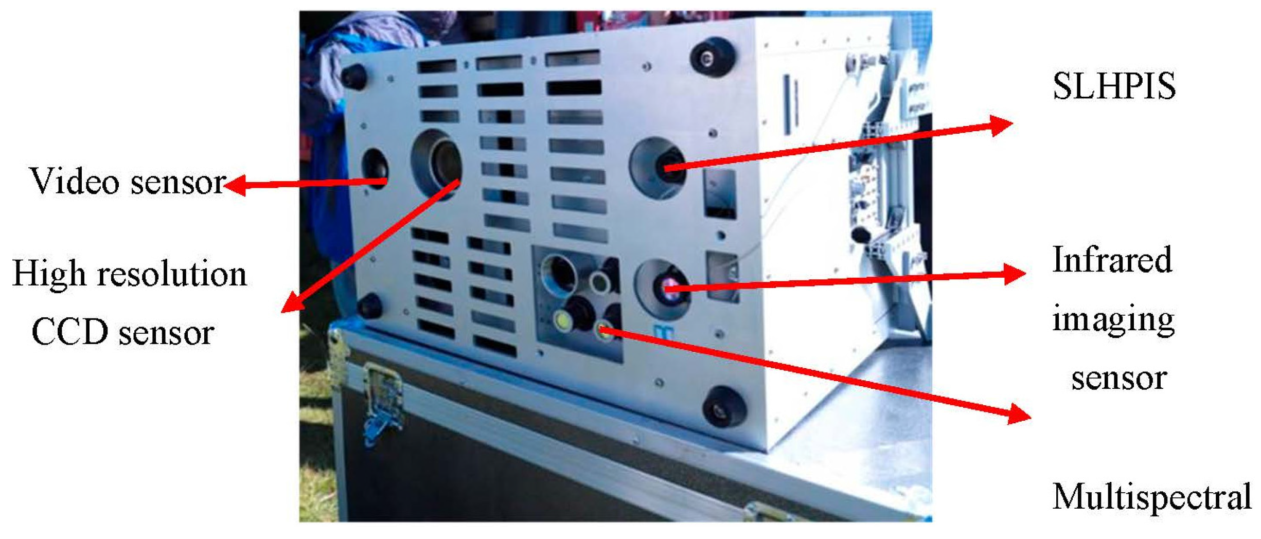
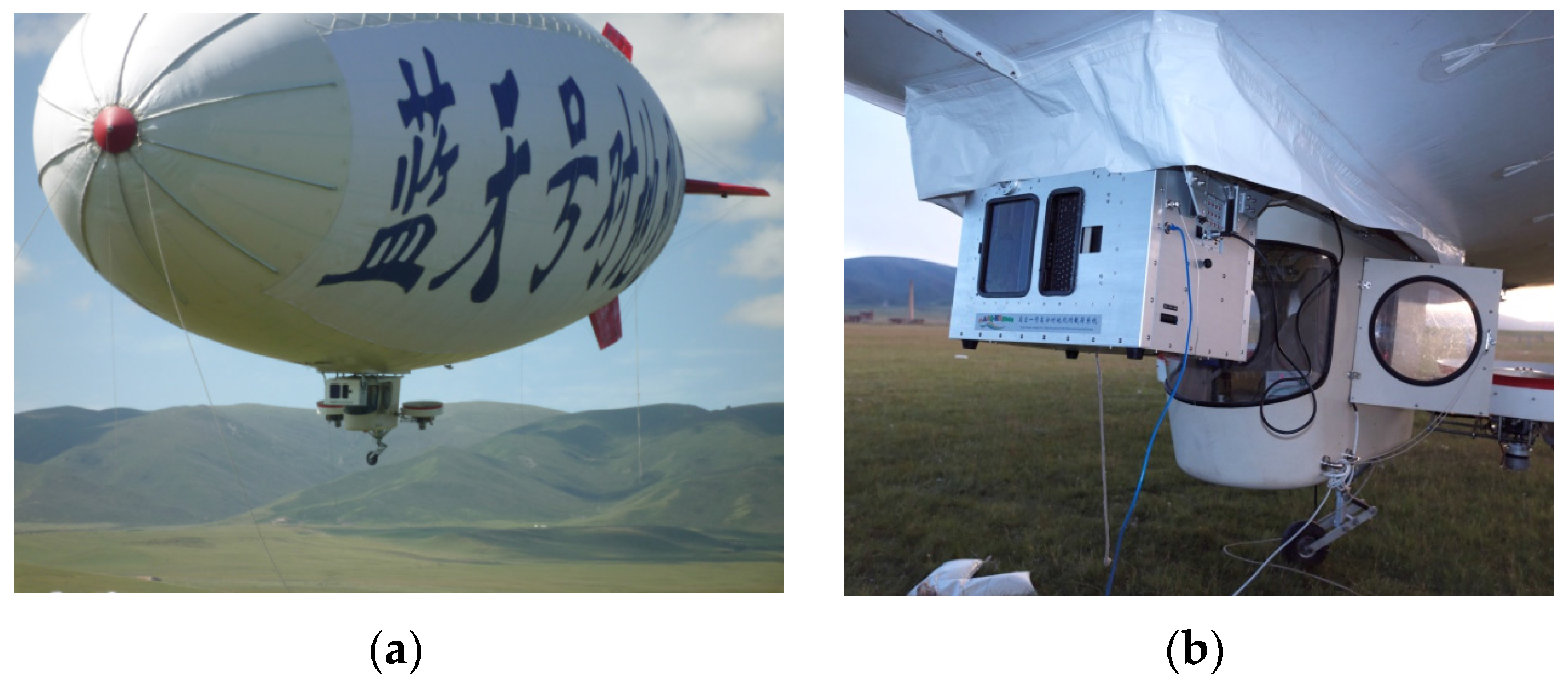
In this paper, a SLHPIS and other five sensors (including high-resolution CCD sensor, infrared sensor, video sensor, and multispectral imaging sensor, POS) are integrated into the HAA Earth observation payload system developed by our research team—“LanTianHao” (in Figure 1a,b). In order to save development costs, “LanTianHao” Earth observation payload system (“LanTianHao” EOPS, in Figure 2) is directly hung under the “LanTianHao” HAA without three-axis stabilized platform. “LanTianHao” HAA platform is 38 meters long and 12 meters high, and is a large soft aerostat. Due to the lack of a three-axis stabilized platform and the air pressure, temperature, and airflow influence at the plateau, the large pitch and roll angles frequently tends to appear. The single linear hyperspectral pushbroom imaging based on “LanTianHao” HAA is much more complex than that of based on spaceborne and airborne [12,13]. The original hyperspectral pushbroom images obtained based on “LanTianHao” HAA are always characterized by severe geometric distortions with the repeated and missing sampling, it is quite problematic to use conventional in-flight calibration methods directly. Furthermore, fewer corresponding points between the images from linear imaging sensor restrict the usage of block adjustment method to calculate the boresight misalignments. Thus, there is a dire need for a new ground-based boresight calibration method for SLHPIS.

Figure 1. (a) “LanTianHao” HAA navigated at an altitude above 4100 m with a payload greater than 200 kg; and (b) docking of “LanTianHao” HAA and “LanTianHao” EOPS.

Figure 1. (a) “LanTianHao” HAA navigated at an altitude above 4100 m with a payload greater than 200 kg; and (b) docking of “LanTianHao” HAA and “LanTianHao” EOPS.

Figure 2. “LanTianHao” EOPS.

Figure 2. “LanTianHao” EOPS.

A literature survey reveals that some studies on the in-flight boresight calibration of SLHPIS [6,14,15,16,17,18] do not comprehensively detail a model for the boresight calibration. As a result, the boresight calibration can hardly be done using these available methods. Yeh et al. [19] has proposed a new direct georeferencing (DG) self-calibration method for SLHPIS. This method requires the calculation of 19 parameters, including boresight misalignments. The pushbroom hyperspectral system employs high precision POS and is installed on a three-axis stabilized platform which results in little distortion to the original hyperspectral pushbroom images. However, this method requires many more ground control points (GCPs) and uses in-flight boresight calibration which is very expensive. The ground-based boresight calibration method [9,20] is a promising alternate approach. However, some of these methods [9] focus on ground mobile LiDAR mapping systems, and some methods [20] focus on frame imaging sensors. There are hardly any methods for the ground-based boresight calibration of SLHPIS.

“LanTianHao” EOPS requires a calibration method based on its own characteristic features. This paper proposes a new ground-based boresight calibration method (named as GBC) for orthorectifying single linear pushbroom hyperspectral images. In our proposed method, first, a detailed calculation procedure for the direct georeferencing (DG) of image point based on POS data is described. Secondly, a boresight calibration model for SLHPIS is put forwarded in accordance with the collinearity equation. Lastly, a group of experiments namely, simulation-based, ground-based, and flight-based experiments, are performed to verify the accuracy and stability of our proposed method for boresight calibration.

2. Direct Georeferencing Based on POS

2.1. Linear Imaging Sensor Exterior Orientation Elements

The linear pushbroom imaging depends on motion of the body platform because every image is only a scan line. First of all, we need to know the external orientation elements of each scan line for orthorectification. These exterior orientation elements of the linear imaging sensor include three orientation angular elements (ω, φ, and κ) and three positional elements (X_s, Y_s, and Zs). The original POS data record the position and orientation of the body platform. The positional data contains WGS84 coordinates (latitude B, longitude L, and ellipsoidal height H) and the orientation data includes all rotational angles between the navigation coordinate system and the body coordinate system (φ, θ, and ψ). After a series of coordinate transformations, these data are transformed from the linear imaging sensor coordinate system to the mapping coordinate system, until the six exterior orientation elements of the linear imaging sensor are obtained. This coordinate transformation is a complicated process and involves five coordinate systems: (i) the coordinate system of linear imaging sensor (B); (ii) the body coordinate system (b); (iii) the local navigation coordinate system (n); (iv) the Earth-center fixed coordinate system (e); and (v) the mapping coordinate system (m).

The transitional matrix obtained by the transformation of the linear imaging sensor coordinate system to the mapping coordinate system is as follows:

$$R_B^m=R_e^m{R}_{n_i}^e{R}_b^{n_i}{R}_B^b=\left[\begin{array}{ccc}{a}_1& a_2& a_3\\ b_1& b_2& b_3\\ c_1& c_2& c_3\end{array}\right]$$

(1)

where $R_B^b$ is the transition matrix from the linear imaging sensor coordinate system to the body coordinate system. $R_b^{n_i}$ is the transition matrix from IMU body coordinate system to the local navigation coordinate system. $R_{n_i}^e$ is the transition matrix from the local navigation coordinate system to the Earth center fixed coordinate system. $R_e^m$ is the transition matrix from the Earth-center fixed coordinate system to the mapping coordinate system.

The positional elements (X_s, Y_s, Z_s)^m can be calculated by considering the level arm matrix $T_B^b$ between the linear imaging sensor coordinate system and IMU body coordinate system. If the origin of the mapping coordinate system in WGS84 coordinate system is (X₀, Y₀, Z₀)^e, then the coordinates of the linear imaging sensor projection center in the mapping coordinate system can be obtained as follows:

$$\left[\begin{array}{c}{X}_S\\ Y_S\\ Z_S\end{array}\right]=R_e^m\left(R_{n_i}^e{R}_b^{n_i}{T}_B^b+{\left[\begin{array}{c}{X}_{POS}\\ Y_{POS}\\ Z_{POS}\end{array}\right]}^e-{\left[\begin{array}{c}{X}_0\\ Y_0\\ Z_0\end{array}\right]}^e\right)$$

(2)

2.2. Geographical Coordinates of Image Points

By using collinearity and matrix Equation (1), geographical coordinates (X, Y) of an image point in the mapping coordinate system can be calculated from Equation (3):

$$\{\begin{array}{c}X-X_s=(Z-Z_s)\frac{a_{1}x+a_{2}y-a_{3}f}{c_{1}x+c_{2}y-c_{3}f}\\ Y-Y_s=(Z-Z_s)\frac{b_{1}x+b_{2}y-b_{3}f}{c_{1}x+c_{2}y-c_{3}f}\end{array}$$

(3)

where Z denotes the elevation of ground control points.

3. Boresight Calibration Model

Ideally, there should be no gap between the assembly of the linear imaging sensor and IMU and the three axes of the IMU coordinate system and the linear imaging sensor coordinate system should be fully aligned in parallel, or at least to keep three known angles (α, β, γ). However, the practical scenario is different. Due to the assembly errors, there are level arms between the origin of the IMU body coordinate system and the linear imaging sensor coordinate system, and also the axes between the IMU body coordinate system and the linear imaging coordinate system were not fully aligned in parallel creating the boresight misalignments (e_x, e_y, e_z). Although the magnitude of the boresight misalignments is very small (generally <1°), these can induce the geographical coordinate errors which can become larger and larger which leads the body platform to rise up.

Taking into account the boresight misalignments, the transformation matrix described by Equation (1) can be revised to Equation (4):

$$R_B^{*m}=R_e^m{R}_{n_i}^e{R}_b^{n_i}{R}_B^b{R}_B^{*b}=R_B^m{R}_B^{*b}=\left[\begin{array}{ccc}{a}_1& a_2& a_3\\ b_1& b_2& b_3\\ c_1& c_2& c_3\end{array}\right]$$

(4)

where $R_B^{*b}$ is a compensated matrix by the boresight misalignments.

The values of the three orientation angles ω, φ, and κ are revised as follows:

$${\mathsf{\omega }}^{*}=\mathsf{\omega }+e_y,{\mathsf{\phi }}^{*}=\mathsf{\phi }+e_x,{\mathsf{\kappa }}^{*}=\mathsf{\kappa }+e_z$$

Some traditional boresight calibration methods for the frame imaging systems can compute the exterior orientation elements using many ground control points (GCPs) and the bundle adjustment. The computed exterior orientation elements are treated as “true” values, and the measured exterior orientation elements by the POS are treated as “observed” values, and then, based on these values, the error equation is formulated. In the next step, the boresight misalignments are calculated based on this formulated error equation. However, because of the imaging characteristics of the linear imaging sensor, these methods cannot be directly applied to calibrate the boresight misalignments for the linear imaging sensor.

There are several other bundle adjustment methods [8,12,21,22,23,24] available for the linear imaging sensor which are totally different from the frame imaging system. In these methods, it is considered that the true values of the exterior orientation elements are made up of the measured values by the POS and the errors which is a function of time e.g., the Polynomial Model.

Taking into account this consideration, the error equation is formulated as follows:

$$\{\begin{array}{l}{X}_s=X_{GPS}+X_0+X_{1}t+X_2{t}^2\hfill \\ Y_s=Y_{GPS}+Y_0+Y_{1}t+Y_2{t}^2\hfill \\ Z_s=Z_{GPS}+Z_0+Z_{1}t+Z_2{t}^2\hfill \\ \mathsf{\phi }={\mathsf{\phi }}_{IMU}+{\mathsf{\phi }}_0+{\mathsf{\phi }}_{1}t+{\mathsf{\phi }}_2{t}^2\hfill \\ \mathsf{\omega }={\mathsf{\omega }}_{IMU}+{\mathsf{\omega }}_0+{\mathsf{\omega }}_{1}t+{\mathsf{\omega }}_2{t}^2\hfill \\ \mathsf{\kappa }={\mathsf{\kappa }}_{IMU}+{\mathsf{\kappa }}_0+{\mathsf{\kappa }}_{1}t+{\mathsf{\kappa }}_2{t}^2\hfill \end{array}$$

(5)

Putting the error equation into the collinearity equation and after linearization, we can obtain exterior orientation elements for each image from linear imaging sensor at the time of exposure by bundle adjustment. However, this method is quite complicated and demands extensive use of many more ground control and checkpoints. Presently, these methods are widely used in orthorectification of multi-line pushbroom imaging system. Owing to the fact that in the single linear imaging sensor the stereo pairs on the same flight line and between the flight lines due to narrow views cannot be obtained, the traditional methods for multi-linear imaging cannot be employed in this scenario to calibrate the boresight misalignments for a single linear hyperspectral imaging sensor.

In a quick and simple boresight calibration for a single linear hyperspectral imaging sensor, some errors, like POS drifts, are ignored by supposing that the true values of the exterior orientation elements are made up of the measured values by the POS and the boresight misalignments. In the next step, the observation equation can be established. The observation and collinearity equations are combined together to formulate the error equation. The boresight misalignments are then calculated by the iterative least squares method and some ground control points (GCPs).

We suppose:

$$\{\begin{array}{l}A=a_{1}x-a_{3}f\\ B=b_{1}x-b_{3}f\\ C=c_{1}x-c_{3}f\end{array}$$

Now the Equation (4) is rewritten as follows:

$$\{\begin{array}{l}X=X_s+(Z-Z_s)\frac{a_{1}x-a_{3}f}{c_{1}x-c_{3}f}=X_s+(Z-Z_s)\frac{A}{C}\\ Y=Y_s+(Z-Z_s)\frac{b_{1}x-b_{3}f}{c_{1}x-c_{3}f}=Y_s+(Z-Z_s)\frac{B}{C}\end{array}$$

(6)

Equation (6) is non-linear in nature and is transformed into a linear form by employing the first-order Taylor expansion. The same is done by calculating the first-order derivatives of the measured values with respect to the observed values. Here, $A_w^{\prime }$ stands for the first-order derivative of A with respect to ω. The new calculated linear formula is described as follows:

$$\{\begin{array}{l}\frac{\partial X}{\partial \mathsf{\phi }}=\frac{\partial X_s}{\partial \mathsf{\phi }}+\frac{\partial (Z-Z_s)}{\partial \mathsf{\phi }}\frac{A}{C}+(Z-Z_s)\frac{A_{\mathsf{\phi }}^{\prime }C-C_{\mathsf{\phi }}^{\prime }A}{C^2}\\ \frac{\partial X}{\partial \mathsf{\omega }}=\frac{\partial X_s}{\partial \mathsf{\omega }}+\frac{\partial (Z-Z_s)}{\partial \mathsf{\omega }}\frac{A}{C}+(Z-Z_s)\frac{A_{\mathsf{\omega }}^{\prime }C-C_{\mathsf{\omega }}^{\prime }A}{C^2}\\ \frac{\partial X}{\partial \mathsf{\kappa }}=\frac{\partial X_s}{\partial \mathsf{\kappa }}+\frac{\partial (Z-Z_s)}{\partial \mathsf{\kappa }}\frac{A}{C}+(Z-Z_s)\frac{A_{\mathsf{\kappa }}^{\prime }C-C_{\mathsf{\kappa }}^{\prime }A}{C^2}\\ \frac{\partial Y}{\partial \mathsf{\phi }}=\frac{\partial Y_s}{\partial \mathsf{\phi }}+\frac{\partial (Z-Z_s)}{\partial \mathsf{\phi }}\frac{B}{C}+(Z-Z_s)\frac{B_{\mathsf{\phi }}^{\prime }C-C_{\mathsf{\phi }}^{\prime }B}{C^2}\\ \frac{\partial Y}{\partial \mathsf{\omega }}=\frac{\partial Y_s}{\partial \mathsf{\omega }}+\frac{\partial (Z-Z_s)}{\partial \mathsf{\omega }}\frac{B}{C}+(Z-Z_s)\frac{B_{\mathsf{\omega }}^{\prime }C-C_{\mathsf{\omega }}^{\prime }B}{C^2}\\ \frac{\partial Y}{\partial \mathsf{\kappa }}=\frac{\partial Y_s}{\partial \mathsf{\kappa }}+\frac{\partial (Z-Z_s)}{\partial \mathsf{\kappa }}\frac{B}{C}+(Z-Z_s)\frac{B_{\mathsf{\kappa }}^{\prime }C-C_{\mathsf{\kappa }}^{\prime }B}{C^2}\end{array}$$

(7)

After considering POS drifts with multiple scanning for the same ground control points, the error equation takes the following form:

$$\{\begin{array}{l}{V}_x={\displaystyle \sum _{i=1}^n(X_{GPS}-({X_0}_i+\frac{\partial X_i}{\partial \mathsf{\phi }}\mathsf{\Delta }\mathsf{\phi }+\frac{\partial X_i}{\partial \mathsf{\omega }}\mathsf{\Delta }\mathsf{\omega }+\frac{\partial X_i}{\partial \mathsf{\kappa }}\mathsf{\Delta }\mathsf{\kappa }))}\\ V_y={\displaystyle \sum _{i=1}^n(Y_{GPS}-({Y_0}_i+\frac{\partial Y_i}{\partial \mathsf{\phi }}\mathsf{\Delta }\mathsf{\phi }+\frac{\partial Y_i}{\partial \mathsf{\omega }}\mathsf{\Delta }\mathsf{\omega }+\frac{\partial Y_i}{\partial \mathsf{\kappa }}\mathsf{\Delta }\mathsf{\kappa }}))\end{array}$$

(8)

where V_x and V_y stand for observation errors, X_GPS and Y_GPS stand for the measured values of the ground control points by RTK-GPS, and n stands for the number of times the ground control points are observed.

Since linearization of the error equation is conducted using the first-order Taylor expansion formula, the iteration is needed for calculating unknown parameters. Let Δφ, Δω, Δκ be the accumulating misalignment angles in each iteration. Their initial values are set to (0, 0, 0) and final corrected values are represented by (e_x, e_y, e_z) which are obtained when the iteration is converged. The relationship established is as under:

$$\{\begin{array}{l}{e}_x^{j+1}=e_x^j+\mathsf{\Delta }\mathsf{\phi }\\ e_y^{j+1}=e_y^j+\mathsf{\Delta }\mathsf{\omega }\\ e_z^{j+1}=e_z^j+\mathsf{\Delta }k\end{array}$$

(9)

where $A_x^{j+1}$ indicates the accumulation value for j + 1 times, Δφ is the corrected factor of φ. The same notation is repeated for Δω and Δκ.

4. Experimentation and Analysis

The proposed GBC method is demonstrated by three sets of tests: simulation test, ground test, and the application on real images from “LanTianHao”. Simulation tests are designed to verify the stability and reliability of the proposed method, and to further investigate the measurement accuracy and effect of GCPs and the number of GCPs, respectively, on the boresight calibration. Ground-based testing is designed to address misalignment problems and checking the results of the boresight calibration. Lastly, the proposed method is validated on the orthorectification of the real hyperspectral pushbroom images from “LanTianHao”.

4.1. Simulation Experiment

In order to verify GBC, a set of simulation-based experiments is done. The simulation experiments were composed of three testing groups with each group containing seven points. By using the focal length of 23 mm for SLHPIS, relative flight altitude of 1000 m and the level arms of 1 m length each, the boresight misalignments based on the actual conditions were calculated out to be 0.7°, 0.6°, and 0.8°. Twenty-one GCPs were generated on the flight-line area.

The 21 GCPs were divided into three groups: seven GCPS in each group and 100 simulation experiments for each group. During the simulation experimentation, the random positional errors (<1 m) were added both to the coordinates of GCPs and the measured coordinates by POS, and the random angle errors (roll errors <0.01°, pitch errors <0.01°, yaw errors <0.05°) were added to the measured angles by POS. In order to test the robustness of the boresight calibration method proposed, large random location errors are introduced intentionally. The detailed experimental results are shown in Table 1. The results indicate that maximum, minimum, and RMSEs for all the three groups are in close match with each other (maximum error ≤ 2′). When the position error is less than 1 m, minimum RMSEs of e_x, e_y, e_z, are up to 0.1724’, 0.1447’, 0.6861’ respectively. The values of e_x, e_y, are very close, but they are lower than e_z. Due to the varying range of the three orientation angles (roll, pitch, and yaw) being different, the varying range of roll and pitch are quite close while they are different in the case of the yaw angle. The reduced errors are obtained from all the three groups. The close match of error results, minimum boresight misalignments, and match of varying range of roll and pitch angles altogether show the perfect viability of the proposed calibration model.

Table 1. Calibration Results.

	Max Error (′)			Min Error (′)			RMSE (′)
	ex	ey	ez	ex	ey	ez	ex	ey	ez
Group1	0.3632	0.6435	2.6056	0.0026	0.0029	0.0229	0.1724	0.1843	0.7620
Group2	0.6924	0.6346	2.8158	0.0090	0.0032	0.0055	0.2471	0.1592	0.8600
Group3	0.6622	0.5681	2.2952	0.0008	0.0011	0.0052	0.2035	0.1447	0.6861

Table 1. Calibration Results.

	Max Error (′)			Min Error (′)			RMSE (′)
	ex	ey	ez	ex	ey	ez	ex	ey	ez
Group1	0.3632	0.6435	2.6056	0.0026	0.0029	0.0229	0.1724	0.1843	0.7620
Group2	0.6924	0.6346	2.8158	0.0090	0.0032	0.0055	0.2471	0.1592	0.8600
Group3	0.6622	0.5681	2.2952	0.0008	0.0011	0.0052	0.2035	0.1447	0.6861

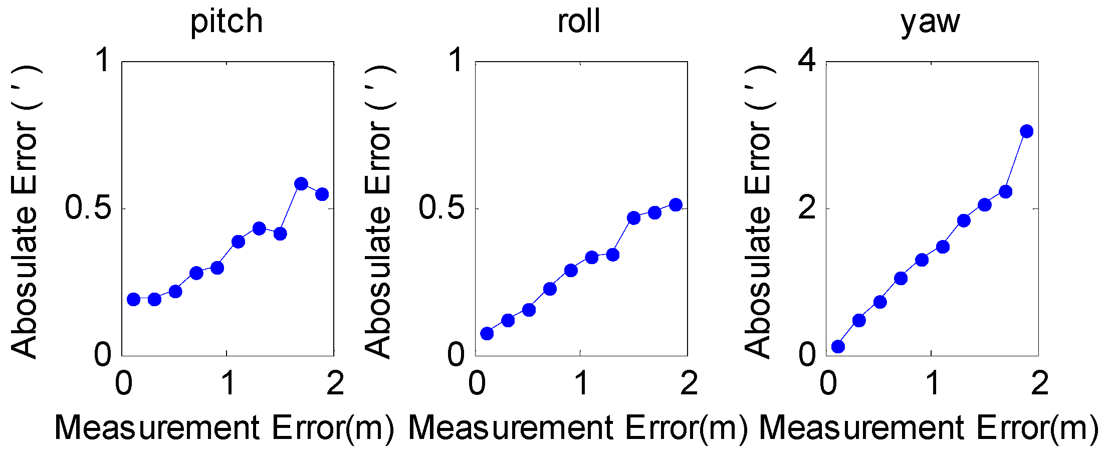
In order to test the effects of measurement error on the calibration results, 20 GCPs were randomly selected while the measurement errors were changed from 0.1 m to 2 m. The average boresight misalignments for 100 experiments were recorded. As shown in Figure 3, the misalignments increase with the increase in measurement error. It shows that the measurement error has a big impact on the boresight calibration. Therefore, to avoid the effect of measurement errors, the GCPs are measured by GPS Real-Time Kinematics.

Figure 3. The boresight misalignments vs. the measurement errors.

Figure 3. The boresight misalignments vs. the measurement errors.

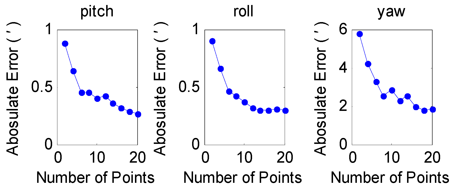
The effect of number of GCPs on the boresight calibration was investigated by assuming the measurement errors to be <1 m, and the number of GCPs ranges from two to 20 (at least two GCPs are needed). The average of the boresight misalignments for 100 experiments was recorded (the random measurement errors <1 m are added into each experiment). The boresight calibration results shown in Figure 4 indicate that the misalignments were enormous with two GCPs. If the GCPs were increased, then the misalignments were decreased drastically. If the control points are increased to a higher number, then the misalignment change is stabilized.

Figure 4. The boresight misalignments vs. the number of control points.

Figure 4. The boresight misalignments vs. the number of control points.

4.2. Ground Calibration Experiment

Bumker [20] had executed the boresight calibration of the frame imaging sensor in the lab and the scan distance from sensor to the ground was kept to about 7 m. Thus, in order to increase the scan distance between the sensor and measured area, the side-scan mode is selected in this paper. “LanTianHao” EOPS including linear hyperspectral imaging sensor was fixed on a tricycle to capture the raw pushbroom images. The raw pushbroom images include the playground of Capital Normal University and some the buildings. The buildings were about 450 m from “LanTianHao” EOPS, and the 12 ground control points (GCPs) were placed at different distance from “LanTianHao” EOPS. The coordinates of GCPs were measured by GPS Real-Time Kinematic (measurement error <1 mm). Differential GPS techniques were adopted to correct bias errors of POS at one location with the synchronized observation data of the GPS base station. The level arms between IMU and the linear hyperspectral imaging sensor were calculated by designed sizes as shown in the mounted schematic. In this paper, like in the flying mode, the tripod traveled at a constant speed back and forth. The technical parameters of the linear hyperspectral imaging sensor and POS in “LanTianHao” EOPS are shown in Table 2. The POS used in this system is SPAN-CPT which is associated to the low precision of POS.

Table 2. The technology parameters of linear hyperspectral imaging sensor and POS.

Linear Hyperspectral Imaging Sensor		POS
Frame Rate	33 fps	Yaw Accuracy	0.05°
Band Number	840	Pitch Accuracy	0.015°
Space Resolution (pixel)	1600	Roll Accuracy	0.015°
Field View Angle	27°	DGPS	1 mm + 1 ppm
		Sample Rate	100 Hz

Table 2. The technology parameters of linear hyperspectral imaging sensor and POS.

Linear Hyperspectral Imaging Sensor		POS
Frame Rate	33 fps	Yaw Accuracy	0.05°
Band Number	840	Pitch Accuracy	0.015°
Space Resolution (pixel)	1600	Roll Accuracy	0.015°
Field View Angle	27°	DGPS	1 mm + 1 ppm
		Sample Rate	100 Hz

There were three methods to calculate the boresight misalignments. The first method is based on using GBC with side-scan mode by 7 GCPs (called SS-7), second method is based on using GBC with side-scan mode by 12 GCPs (called SS-12), and the third method is based on using GBC with the toward-ground scanning mode (called TGS). To examine the calculated boresight misalignments, the 12 GCPs were looked as the checkpoints. We inputted the original POS data and the boresight misalignments calculated using the three methods into Equation (4) to compute the geographical coordinates of the checkpoints, respectively. They were compared with the coordinates of 12 GCPs from the GPS Real-Time Kinematics separately. The comparison of the results is shown in Table 3. The non-calibration indicates that the calculated boresight misalignments were not inputted into the Equation (4).

Table 3. Quality of boresight calibration.

Method	RMSEx (m)	RMSEz (m)	RMSEx-z (m)
Un-calibration	0.6475	1.2497	0.9952
GBC (SS-7)	0.1239	0.0997	0.1124
GBC (SS-12)	0.1093	0.0987	0.1041
TGS	0.3391	0.7570	0.5865

Table 3. Quality of boresight calibration.

Method	RMSEx (m)	RMSEz (m)	RMSEx-z (m)
Un-calibration	0.6475	1.2497	0.9952
GBC (SS-7)	0.1239	0.0997	0.1124
GBC (SS-12)	0.1093	0.0987	0.1041
TGS	0.3391	0.7570	0.5865

The positional errors (RMSEx–z) of SS-7 is reduced from 0.9952 to 0.1124 m. The positional errors (RMSEx–z) of SS-12 is reduced from 0.9952 to 0.1041 m. The positional error (RMSEx–z) of TGS is 0.5865 m. As a result, the solutions of our ground-based boresight calibration with the side-scanning mode are reliable for rectifying pushbroom images, including the distant objects, and the positional errors from SS-7 and SS-12 are very close. However, the ground-based boresight calibration with the toward-ground scanning mode is not reliable for rectifying pushbroom images including the distant objects, since the scanning distance between the sensor and the measured area is short while calibrating the boresight misalignments.

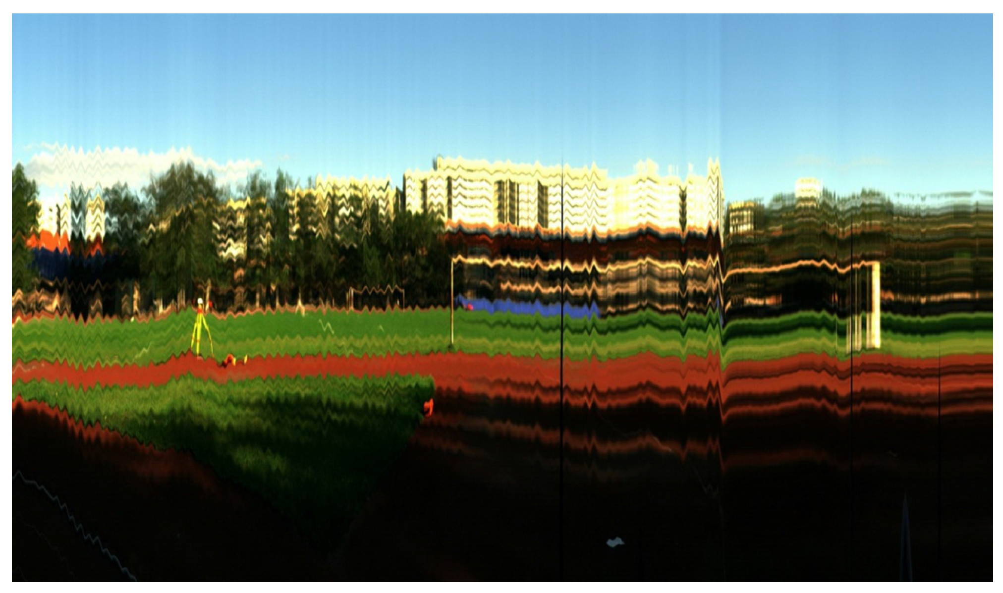
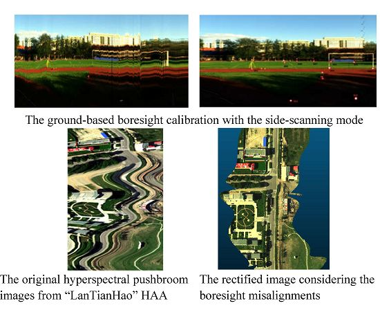
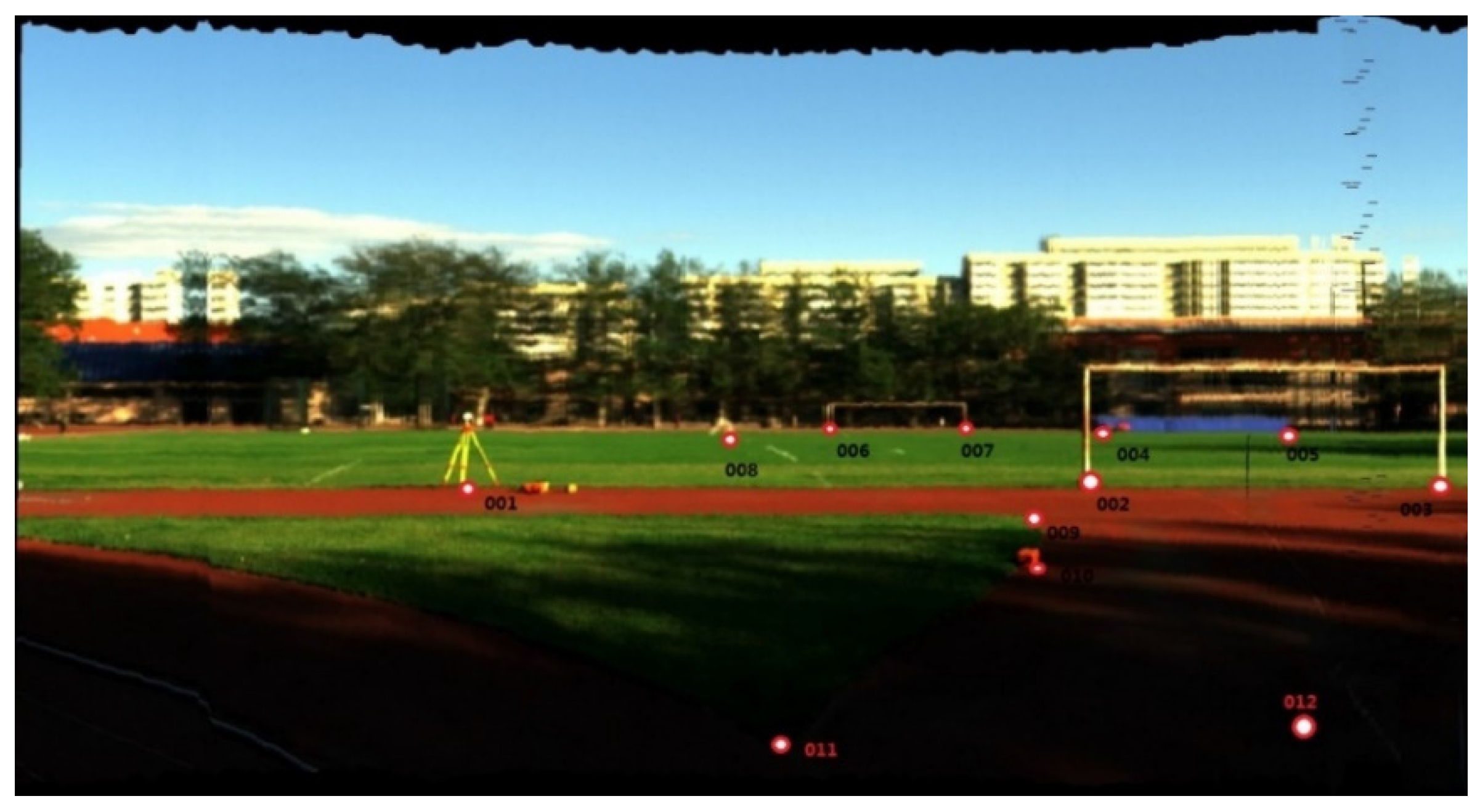
Figure 5 is the raw image acquired by GBC with the side-scanning mode, the raw image includes geometric distortions. Figure 6 shows the rectified image by the GBC (SS-12) approach, and the 12 CGPs are marked on it. The positional errors of 12 CGPs on the rectified image are different because of different scan distance. Table 4 shows the analysis of the change of the positional errors with respect to the scan distance. The 12 CGPs are placed at different distances. The positional errors of the CGPs become bigger as the scan distance increases. At the scan distance of about 30 m, the positional error (Dx–z) of SS-12 is 0.0337 m; At the scan distance of about 200 m, the positional error (Dx–z) of SS-12 is 0.1322 m. While calibrating the boresight misalignments, the CGPs were placed on the ground. So the correlation among the CGPs, the level arm offsets and boresight misalignments cannot be computed together. In the future, the CGPs can be fixed uniformly on the facades of the buildings and the scanning distance is best to equalize the relative flight height while calibrating the boresight misalignment angles.

Figure 5. The raw image acquired by GBC with the side-scanning mode. (it includes geometric distortions).

Figure 5. The raw image acquired by GBC with the side-scanning mode. (it includes geometric distortions).

Figure 6. The rectified result with boresight calibration (the 12 CGPs are marked on it).

Figure 6. The rectified result with boresight calibration (the 12 CGPs are marked on it).

Table 4. The change of the positional errors with scan distance.

Scanning Distance	Before Calibration	After Calibration
	Dx-z/m	Dx-z/m
About 30 m	0.2840	0.0337
About 100 m	1.7394	0.0918
About 200 m	2.2492	0.1322

Table 4. The change of the positional errors with scan distance.

Scanning Distance	Before Calibration	After Calibration
	Dx-z/m	Dx-z/m
About 30 m	0.2840	0.0337
About 100 m	1.7394	0.0918
About 200 m	2.2492	0.1322

4.3. In-Flight Experimentation

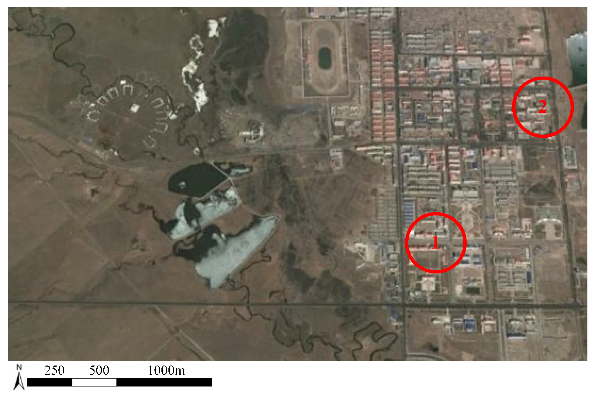
In August 2014, we did in-flight experiments using “LanTianHao” in Jinyintan grassland with an average altitude above 3700 m, Qinghai province, as shown in Figure 7. “LanTianHao” HAA navigated at an altitude of more than 4100 m with a payload of more than 200 kg (Figure 1a). In order to save the development cost, “LanTianHao” EOPS was directly installed under the “LanTianHao” HAA without the three-axis stabilized platform (Figure 1b). 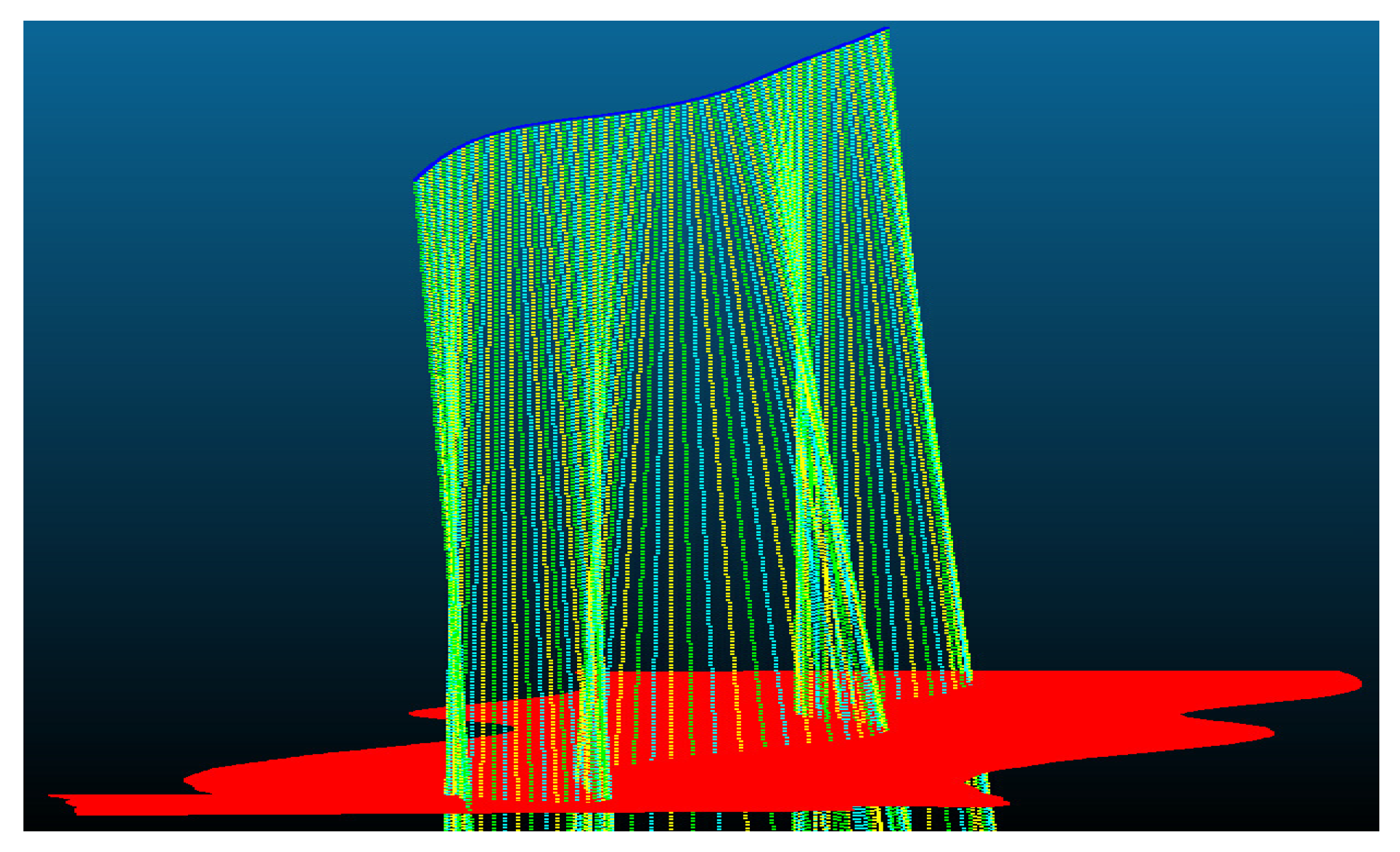The payload of “LanTianHao” EOPS is shown in Figure 2. The altitude change of the airship directly affects the original hyperspectral pushbroom images. 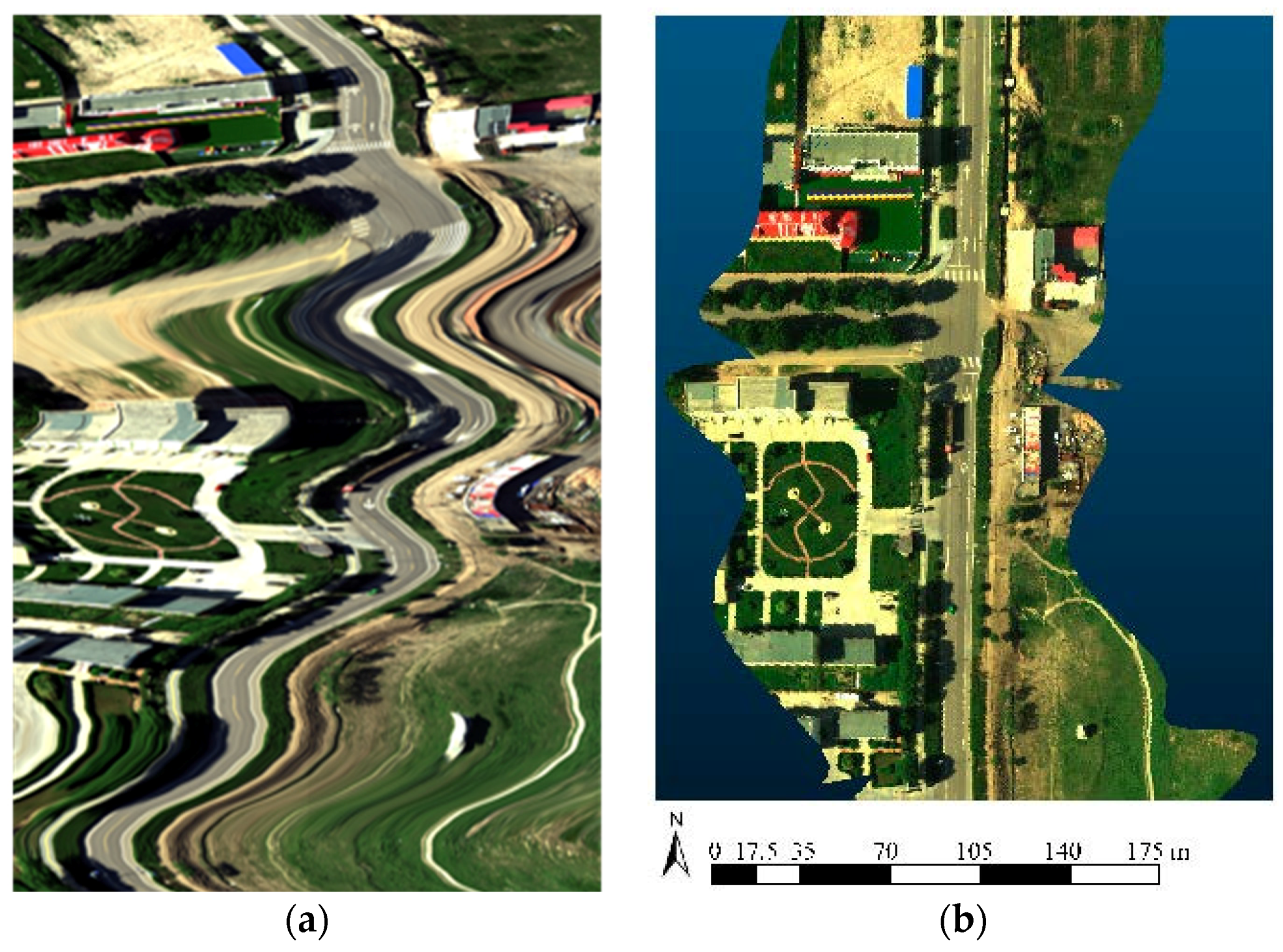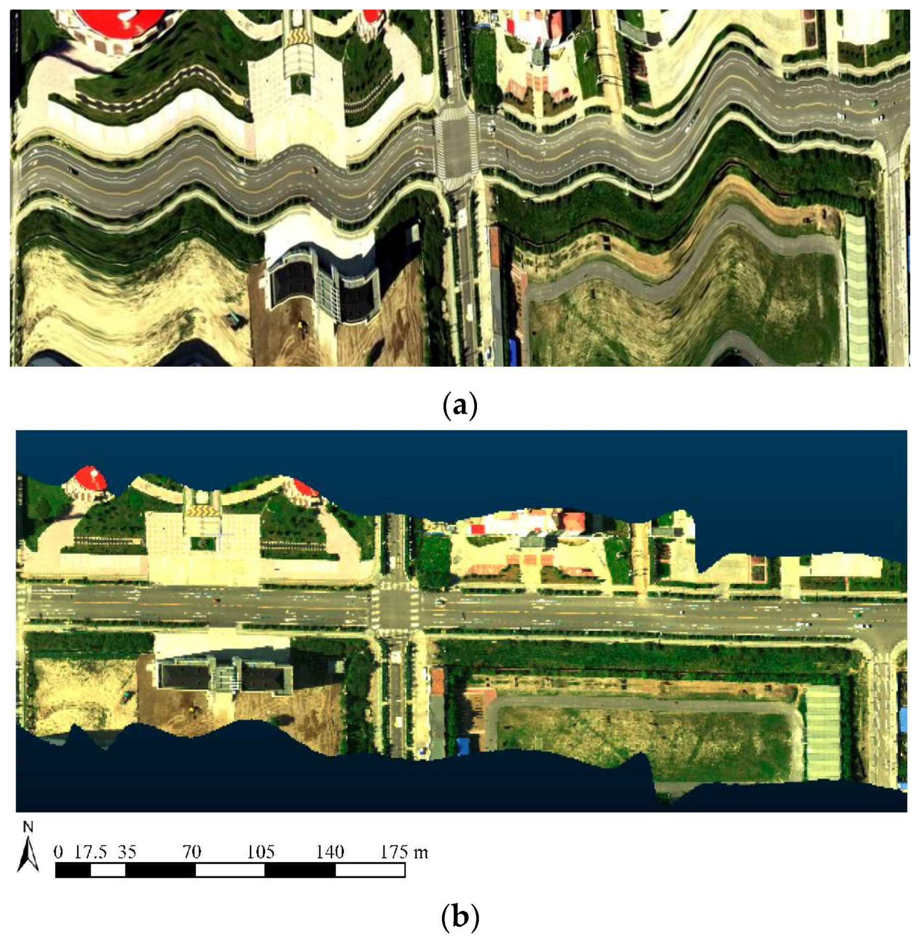Due to the large pitch angles, some scan lines are crossing as shown in Figure 8 owing to the repeated and missed sampling, alternatively. Due to the large roll angles, the original pushbroom hyperspectral images are seriously distorted as depicted in Figure 9a and Figure 10a. In such a case, it is necessary to perform boresight calibration on the ground level. The results (SS-7 and SS-12) of boresight calibration on the ground shown in Section 4.2 were inputted into the linear pushbroom imaging correction Equation (4), respectively. Figure 9b and Figure 10b show the rectified results by SS-7 in 0.096 m ground sample distance (GSD) of hyperspectral pushbroom imaging after boresight misalignments compensation step. Figure 9 corresponds Circle 1 in Figure 7; Figure 10 corresponds Circle 2 in Figure 7.

Figure 7. Study Area: the Jinyintan grassland, Qinghai, China. The imagery is from Google Earth.

Figure 7. Study Area: the Jinyintan grassland, Qinghai, China. The imagery is from Google Earth.

Figure 8. The repeated and missed sampling, alternatively, due to the large pitch and roll angles frequently appearing.

Figure 8. The repeated and missed sampling, alternatively, due to the large pitch and roll angles frequently appearing.

Figure 9. (a) The original hyperspectral pushbroom images from “LanTianHao” HAA; and (b) the rectified image by SS-7.

Figure 9. (a) The original hyperspectral pushbroom images from “LanTianHao” HAA; and (b) the rectified image by SS-7.

Figure 10. (a) The original hyperspectral pushbroom images from “LanTianHao” HAA; and (b) the rectified image by SS-7.

Figure 10. (a) The original hyperspectral pushbroom images from “LanTianHao” HAA; and (b) the rectified image by SS-7.

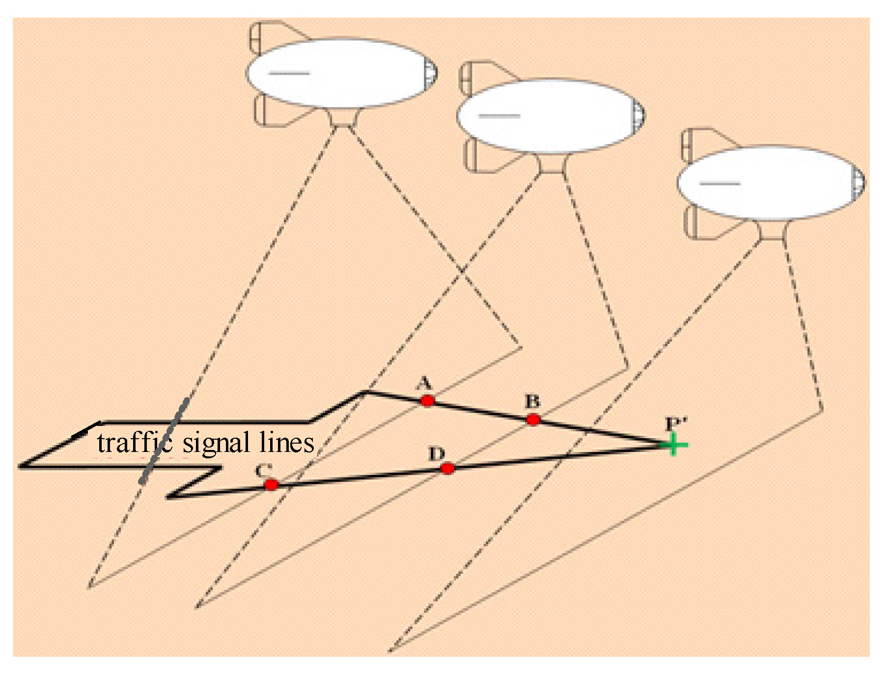
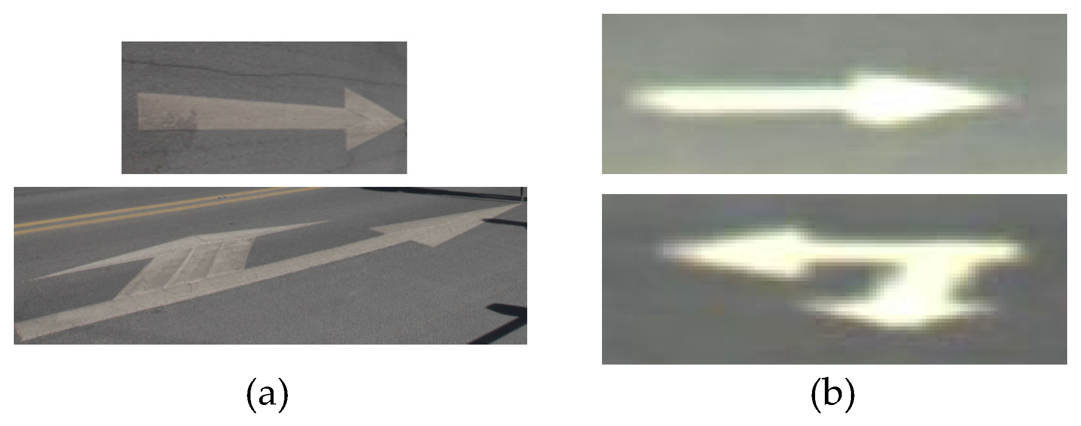
In order to test the ground location accuracy of the image points, the cross points of the ground traffic signal lines were regarded as the checkpoints needed to test the hyperspectral pushbroom orthorectification after boresight calibration. While during the data processing, we first computed the geographical coordinates of A, B, C, and D, and then calculated the geographical coordinates of cross point “P” in order to reduce the errors caused by sampling, as shown in Figure 11. The calculated coordinates of point “P” were compared with the measured coordinates of point “P” by GPS-RTK.

The coordinates of checkpoints were measured by GPS-RTK (like Figure 12a). The coordinates of checkpoints were calculated on the rectified images (like Figure 12b). Twenty checkpoints of traffic signs were selected in test area to calculate the positional error (RMSE_X–Y). The positional error (RMSE_X–Y) is nearly close to 0.2 m while GSD of our hyperspectral imaging sensor is 0.096 m and the relative flight height is around 300 m, so an error of 0.2 m is treated equal to two pixels. The positional error can meet most applications.

Figure 11. Computing coordinates of checkpoints using ground traffic signs.

Figure 11. Computing coordinates of checkpoints using ground traffic signs.

Figure 12. The selected traffic signs ((a) measuring the checkpoints of traffic signs; (b) the enlarged traffic signs on the retcified images).

Figure 12. The selected traffic signs ((a) measuring the checkpoints of traffic signs; (b) the enlarged traffic signs on the retcified images).

According to the results of the linear hyperspectral imaging orthorectification in Figure 9b and Figure 10b, the ground traffic signal lines and the edges of houses are in a straight line which shows the viability of the proposed method.

5. Discussions

Some experiments based on simulation, ground and flight were used in solving and validating our ground-based boresight calibration approach. In the simulation experiments, we validated the effects of measurement error and quantity of GCPs on the calibration results. The measurement error of GCPs has a significant impact on the boresight calibration, so the GCPs should be measured by GPS Real-Time Kinematics. The number of GCPs is not the more the better; there is an upper limit. In the ground-based experiments, we did some comparisons of different scanning distance. The positional errors can become larger as the scanning distance increases, so the relative flight height is best between 300 m and 500 m in the field fight experiments if our ground-based boresight calibration method is applied. In the flight-based on experiments, the positional error (RMSE_X–Y) is nearly close to two pixels in 0.096 m GSD by applying our SS-7 approach. Moreover, the SPAN-CPT POS with low accuracy is used in our system without a three-axis stabilized platform, and so the raw pushbroom images are seriously distorted. On the contrary, Yeh et al. [19] employed a high accuracy Applanix POS AV510 and three-axis stabilized platform. The large pitch and large roll angles hardly appear, and the positional RMSE_X–Y was close to 2.583 m (2.5 pixels) in 1 m GSD.

Although our ground-based boresight calibration method is for the single linear hyperspectral pushbroom imaging system based on high altitude airship (HAA), it can also be applied to some other pushbroom imaging system including based on ground pushbroom imaging system and based on airborne pushbroom imaging system. Furthermore, compared with the in-flight calibration method, the cost of flight experiments can be saved by using our ground-based boresight calibration method.

6. Conclusions

In-flight calibration has been a standard boresight calibration, but in-flight calibration increases the flight cost and field work. Moreover, “LanTianHao” HAA is a large soft aerocraft, the large pitch and roll angles frequently appear because of the influence of the wind and airflow, so in-flight calibration is not suitable for this special case.

In this paper, a new ground-based boresight calibration method for the single linear imaging sensor on the high altitude airship platform was proposed. Our ground-based boresight calibration method is realized by the iterative least squares method using fewer ground control points (GCPs) and ground-based side-scanning experiments.

The simulation experiments show that the ground-based boresight calibration approach is roust. The ground-based experiments show that the side scanning mode is a better scanning mode for the ground-based boresight calibration. The flight-based on experiments show that the positional error is nearly close to two pixels by applying our SS-7 approach. The aforementioned experiments validate that our proposed ground-based boresight calibration approach improves the quality of the georeferencing results in reducing the geometric distortions caused by the boresight misalignments.