
Estimation of Alpine Forest Structural Variables from Imaging Spectrometer Data


Abstract
:
1. Introduction
2. Method
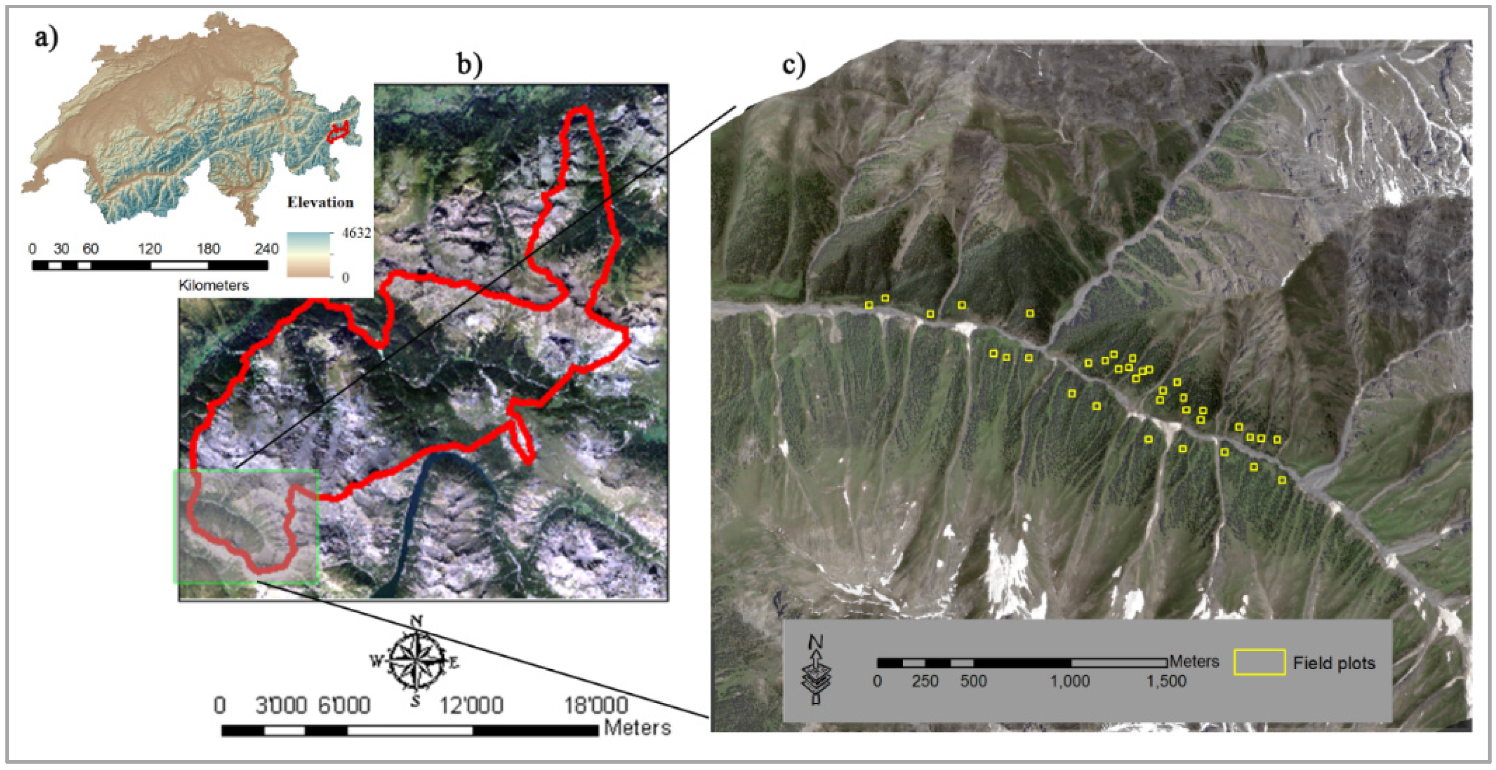
2.1. Study Area

2.2. Field Data
2.3. APEX Imaging Spectrometer Data
2.4. Vegetation Indices
2.4.1. Narrow-Band Vegetation Indices
2.4.2. Band Depth Indices

| Spectral Domain | Location of the Selected Wavelength | ||
|---|---|---|---|
| Start of Spectral Region Analysis (nm) | Center of Spectral Region Analysis (nm) | End of Spectral Region Analysis (nm) | |
| VIS | 653 | 678 | 724 |
| NIR | 1113 | 1179 | 1286 |
| SWIR1 | 1600 | 1707 | 1784 |
| SWIR2 | 2090 | 2211 | 2252 |
2.5. Correlograms
2.6. Regression Analysis
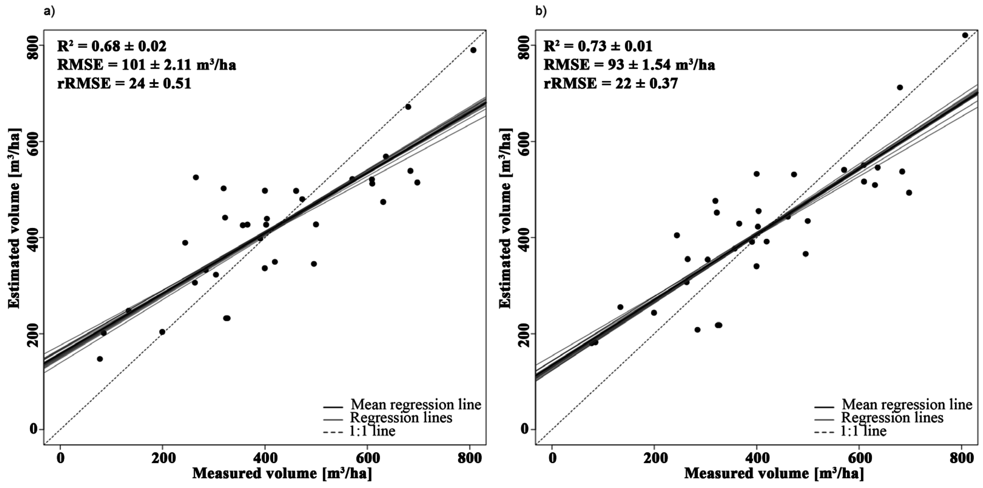
2.7. Validation
3. Results
3.1. In-Situ Forest Structural Measurements
| Parameter | Mean | Minimum | Maximum | SD | CV (%) |
|---|---|---|---|---|---|
| Mean DBH (cm) | 31.9 | 18.62 | 53.5 | 9 | 28 |
| Mean height (m) | 16 | 10.8 | 22.7 | 2.9 | 18 |
| Basal area (m2/ha) | 42.5 | 8.8 | 74 | 16 | 37 |
| Volume (m3/ha) | 421.7 | 77.6 | 807 | 181.7 | 43 |
| Canopy closure (%) | 61 | 22 | 85 | 15.3 | 25 |
3.2. Empirical Models to Estimate Structural Variables
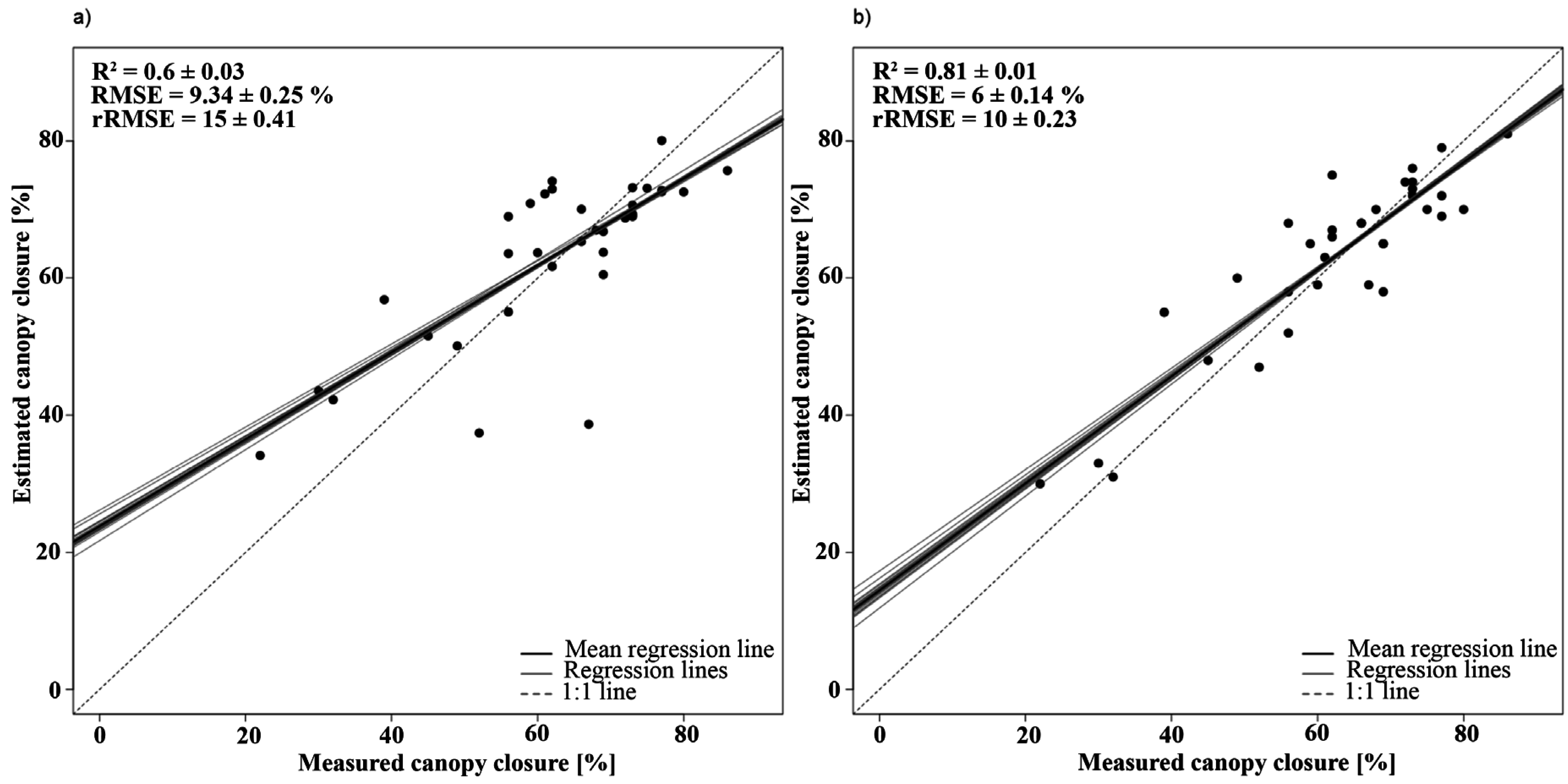
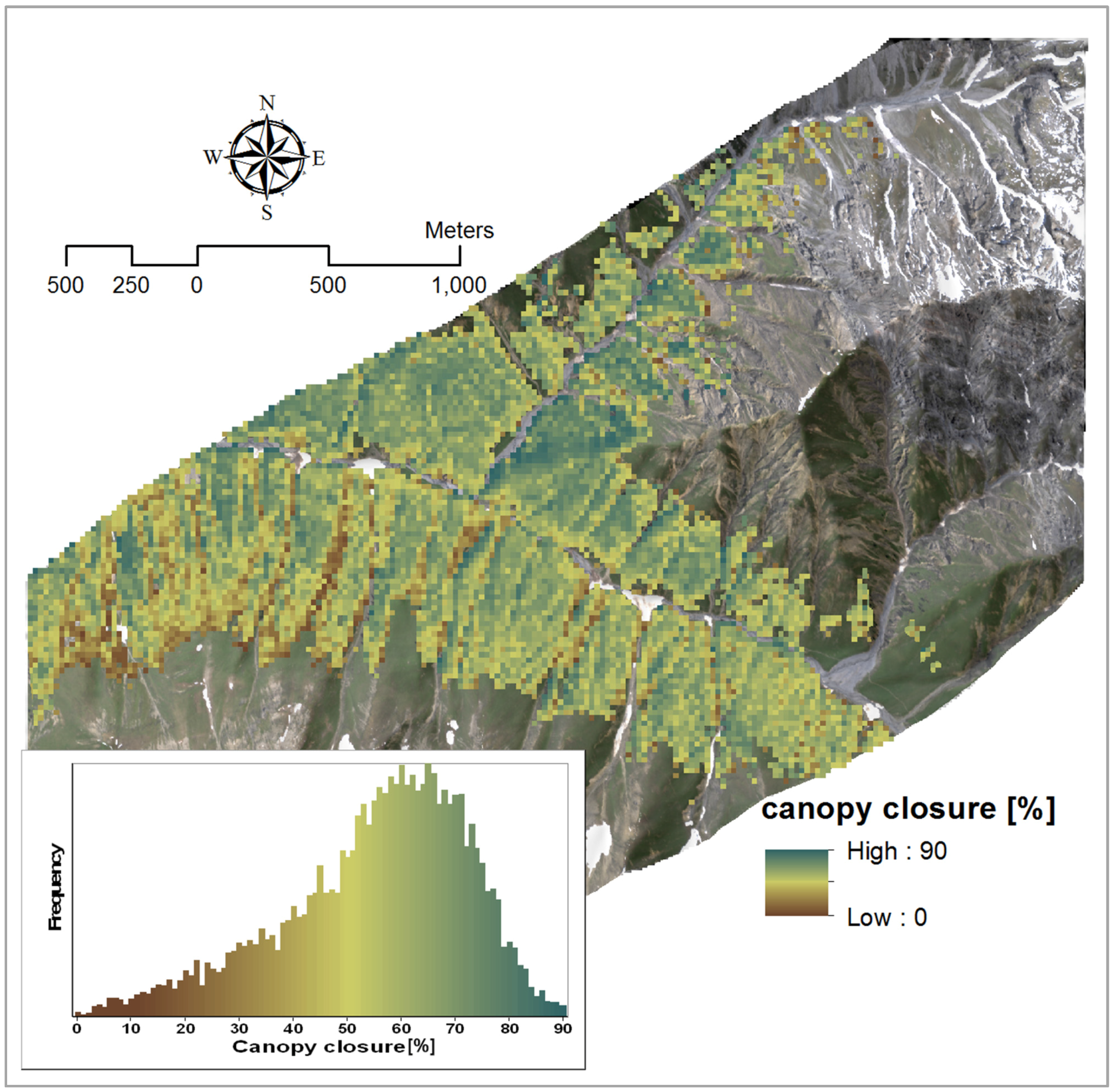
3.2.1. Canopy Closure
| Variable | Model | Wavelength (nm) | R2 | VIF |
|---|---|---|---|---|
| Canopy closure | Y = −0.305 × PVI + 124.57 | 888, 763 | 0.76 | 1 |
| Y = −1372.12 × BDR_NIR − 214.91 × BDR_SWIR2 + 5.33 × AUC_NIR-317.35 × SR + 469.79 | BDR_NIR: 1257 | 0.90 | 1.42 | |
| BDR_SWIR2: 2176 | 1.01 | |||
| AUC: 1113-1286 | 2.95 | |||
| SR: 2253, 2204 | 3.40 |

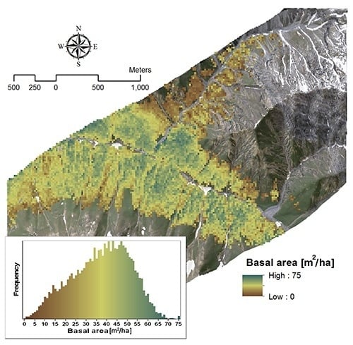
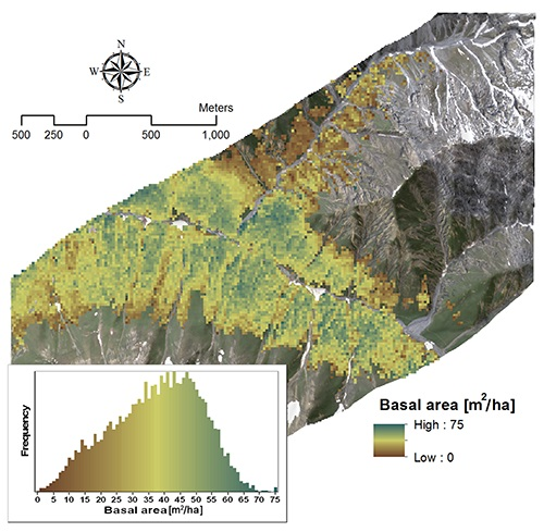
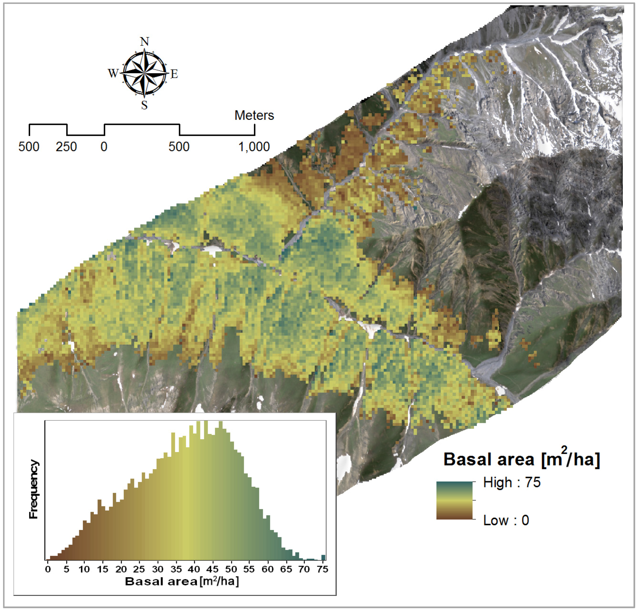
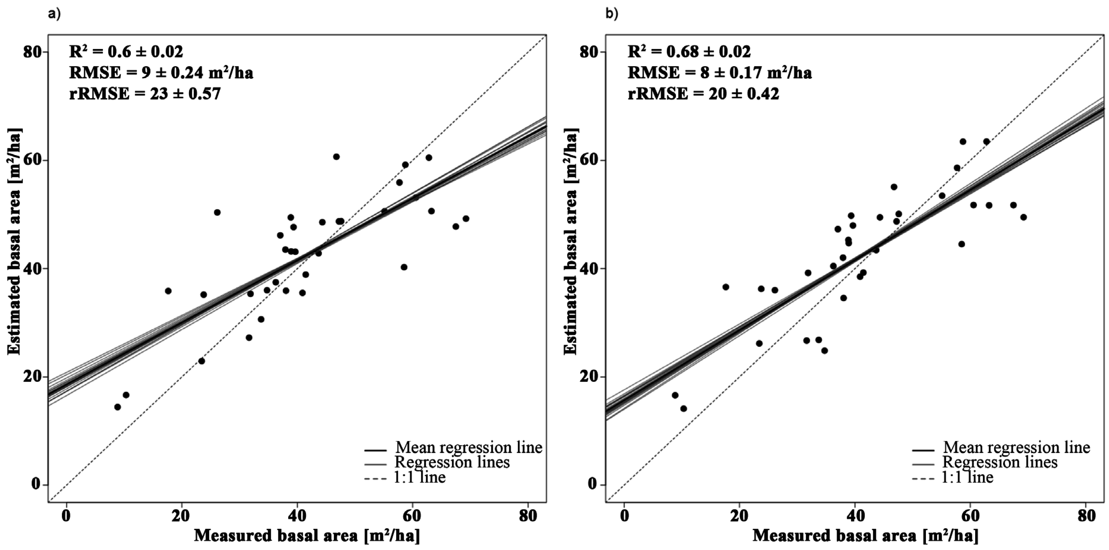
3.2.2. Basal Area
| Variable | Model | Wavelength (nm) | R2 | VIF |
|---|---|---|---|---|
| Basal area | Y = −252.01 × SR + 220.32 | 2385, 1993 | 0.63 | 1 |
| Y = −265.2 × SR − 115.99 × NBDI_SWIR1 + 241.26 | NBDI_SWIR1: 1698 | 0.72 | 1.02 | |
| SR: 2385, 1993 | 1.02 |
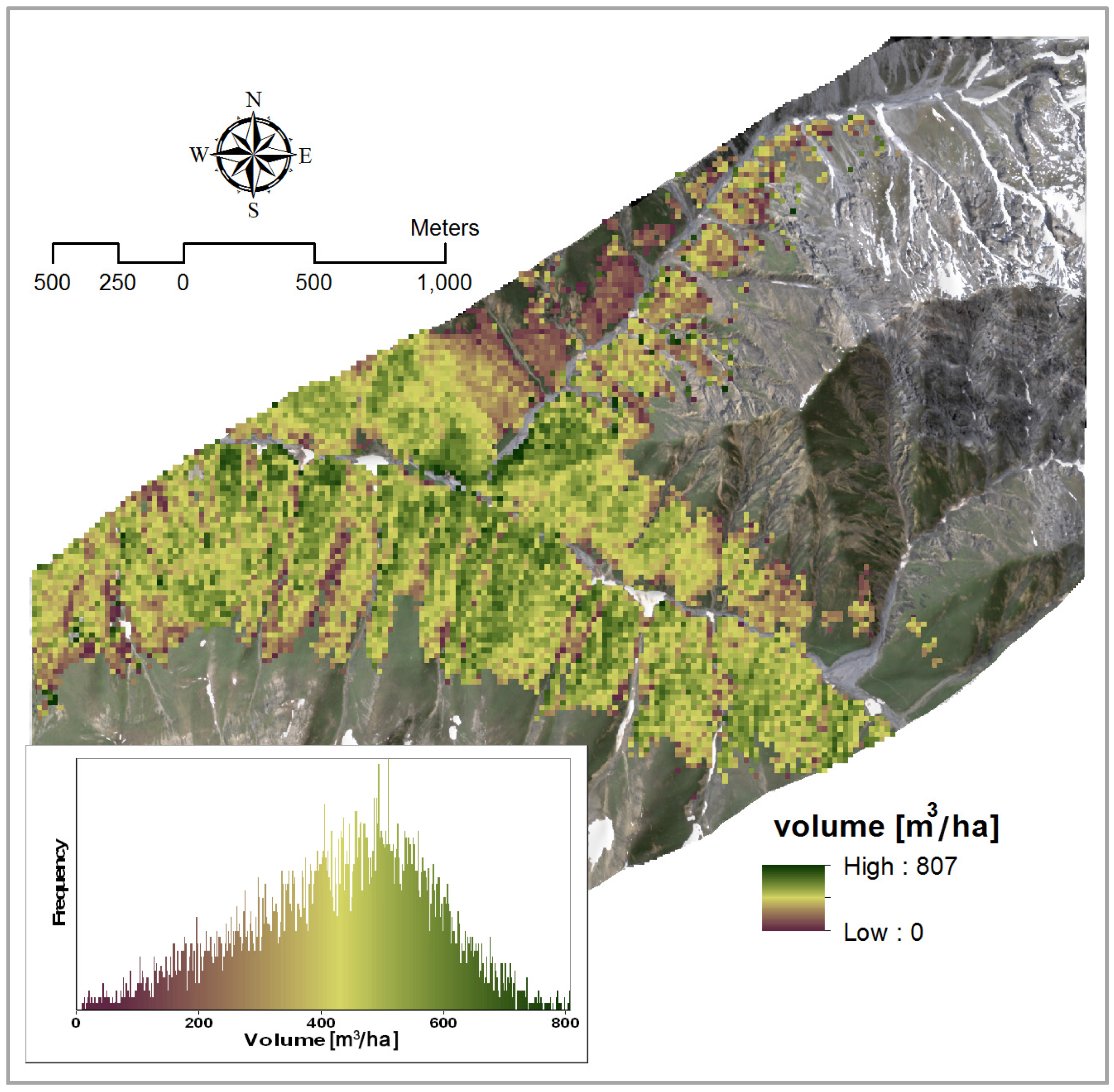
3.2.3. Volume
| Variable | Model | Wavelength (nm) | R2 | VIF |
|---|---|---|---|---|
| Volume | Y = 3.27 × PVI + 59.79 | 1993, 2091 | 0.64 | - |
| Y = −2052.02 × NBDI_SWIR1 + 3.33 × PVI + 185.91 | NBDI_SWIR1: 1698 | 0.72 | 1.03 | |
| PVI: 1993, 2091 | 1.03 |


4. Discussion
4.1. Reliability of Structural Parameter Retrieval from APEX Data
4.1.1. Canopy Closure
4.1.2. Basal Area
4.1.3. Volume
4.2. Reliability of Structural Parameter Retrieval from APEX Data
4.3. Strategies for Improved Simultaneous Retrieval of Biochemical and Structural Plant Traits
5. Conclusions
Supplementary Files
Supplementary File 1Supplementary File 2Supplementary File 3Acknowledgments
Author Contributions
Conflicts of Interest
References
- Kangas, A.; Maltamo, M. Forest Inventory Methodology and Applications; Springer: Amsterdam, The Netherland, 2006. [Google Scholar]
- Hudak, A.T.; Crookston, N.L.; Evans, J.S.; Falkowski, M.J.; Smith, A.M.; Gessler, P.E.; Morgan, P. Regression modeling and mapping of coniferous forest basal area and tree density from discrete-return LiDAR and multispectral satellite data. Can. J. Remote Sens. 2006, 32, 126–138. [Google Scholar] [CrossRef]
- Soenen, S.A.; Peddle, D.R.; Coburn, C.A.; Hall, R.J.; Hall, F.G. Canopy reflectance model inversion inmultiple forward model: Forest structural information retrieval from solution set distributions. Photogramm. Eng. Remote Sens. 2009, 75, 361–374. [Google Scholar] [CrossRef]
- Penman, J.; Michael, G.; Taka, H.; Thelma, K.; Dina, K.; Riitta, P.; Leandro, B. Good Practice Guidance for Land Use, Land-Use Change and Forestry; Institute for Global Environmental Strategies: Hayama, Japan, 2003. [Google Scholar]
- Luther, J.E.; Fournier, R.A.; Piercey, D.E.; Guindon, L.; Hall, R.J. Biomass mapping using forest type and structure derived from Landsat TM imagery. Int. J. Appl. Earth Obs. Geoinf. 2006, 8, 173–187. [Google Scholar] [CrossRef]
- Gil, M.V.; Blanco, D.; Carballo, M.T.; Calvo, L.F. Carbon stock estimates for forests in the Castilla y León region, Spain. A GIS based method for evaluating spatial distribution of residual biomass for bio-energy. Biomass Bioenerg. 2011, 35, 243–252. [Google Scholar] [CrossRef]
- Hall, R.J.; Skakun, R.S.; Arsenault, E.J.; Case, B.S. Modeling forest stand structure attributes using Landsat ETM+ data: Application to mapping of aboveground biomass and stand volume. For. Ecol. Manage. 2006, 225, 378–390. [Google Scholar] [CrossRef]
- Cermák, J.; Nadezhdina, N.; Trcala, M.; Simon, J. Open field-applicable instrumental methods for structural and functional assessment of whole trees and stands. iForest-Biogeo. For. 2014, 40, 1–53. [Google Scholar] [CrossRef]
- Treitz, P.M.; Howarth, P.J. Hyperspectral remote sensing for estimating biophysical parameters of forest ecosystems. Prog. Phys. Geogr. 1999, 23, 359–390. [Google Scholar] [CrossRef]
- Wolter, P.T.; Townsend, P.A.; Sturtevant, B.R.; Kingdon, C.C. Remote sensing of the distribution and abundance of host species for spruce budworm in Northern Minnesota and Ontario. Remote Sens. Environ. 2008, 112, 3971–3982. [Google Scholar] [CrossRef]
- Jakubauskas, M.E.; Price, K.P. Empirical relationships between structural and spectral factors of Yellowstone Lodgepole Pine Forests. Photogramm. Eng. Remote Sens. 1997, 63, 1375–1381. [Google Scholar]
- Hyde, P.; Dubayah, R.; Walker, W.; Blair, J.B.; Hofton, M.; Hunsaker, C. Mapping forest structure for wildlife habitat analysis using multi-sensor (LiDAR, SAR/InSAR, ETM+, Quickbird) synergy. Remote Sens. Environ. 2006, 102, 63–73. [Google Scholar] [CrossRef]
- Schumacher, J.; Christiansen, J.R. Forest canopy water fluxes can be estimated using canopy structure metrics derived from airborne light detection and ranging (LiDAR). Agric. For. Meteorol. 2015, 203, 131–141. [Google Scholar] [CrossRef]
- Ota, T.; Ahmed, O.; Franklin, S.; Wulder, M.A.; Kajisa, T.; Mizoue, N.; Yoshida, S.; Takao, G.; Hirata, Y.; Furuya, N.; et al. Estimation of airborne LiDAR-Derived tropical forest canopy Height using landsat time series in Cambodia. Remote Sens. 2014, 6, 10750–10772. [Google Scholar] [CrossRef]
- Hyyppä, J.; Hyyppä, H.; Inkinen, M.; Engdahl, M.; Linko, S.; Zhu, Y.-H. Accuracy comparison of various remote sensing data sources in the retrieval of forest stand attributes. For. Ecol. Manage. 2000, 128, 109–120. [Google Scholar] [CrossRef]
- Lu, D. The potential and challenge of remote sensing-based biomass estimation. Int. J. Remote Sens. 2006, 27, 1297–1328. [Google Scholar] [CrossRef]
- Gebreslasie, M.T.; Ahmed, F.B.; van Aardt, J.A.N. Predicting forest structural attributes using ancillary data and ASTER satellite data. Int. J. Appl. Earth Obs. Geoinf. 2010, 12, S23–S26. [Google Scholar] [CrossRef]
- Vashum, K.T.; Jayakumar, S. Methods to estimate above-ground biomass and carbon stock in natural forests: A Review. J. Ecosyst. Ecography 2012, 2, 1–7. [Google Scholar] [CrossRef]
- Sivanpillai, R.; Smith, C.T.; Srinivasan, R.; Messina, M.G.; Wu, X.B. Estimation of managed loblolly pine stand age and density with Landsat ETM+ data. For. Ecol. Manage. 2006, 223, 247–254. [Google Scholar] [CrossRef]
- Defibaughy Chávez, J.; Tullis, J.A. Deciduous forest structure estimated with LiDAR-optimized spectral remote sensing. Remote Sens. 2013, 5, 155–182. [Google Scholar] [CrossRef]
- Stojanova, D.; Panov, P.; Gjorgjioski, V.; Kobler, A.; Džeroski, S. Estimating vegetation height and canopy cover from remotely sensed data with machine learning. Ecol. Inform. 2010, 5, 256–266. [Google Scholar] [CrossRef]
- Pu, R.; Gong, P. Wavelet transform applied to EO-1 hyperspectral data for forest LAI and crown closure mapping. Remote Sens. Environ. 2004, 91, 212–224. [Google Scholar] [CrossRef]
- Clevers, J.; Van der Heijden, G.; Verzakov, S.; Schaepman, M.E. Estimating grassland biomass using SVM band shaving of hyperspectral data. Photogramm. Eng. Remote Sens. 2007, 73, 1141–1148. [Google Scholar] [CrossRef]
- Lu, D.; Mausel, P.; Brondı́zio, E.; Moran, E. Relationships between forest stand parameters and Landsat TM spectral responses in the Brazilian Amazon Basin. For. Ecol. Manage. 2004, 198, 149–167. [Google Scholar] [CrossRef]
- Lefsky, M.A.; Cohen, W.B.; Spies, T.A. An evaluation of alternate remote sensing products for forest inventory, monitoring, and mapping of Douglas-fir forests in western Oregon. Can. J. For. Res. 2001, 31, 78–87. [Google Scholar] [CrossRef]
- Lim, K.; Treitz, P.; Wulder, M.A.; St-Onge, B.; Flood, M. LiDAR remote sensing of forest structure. Prog. Phys. Geogr. 2003, 27, 88–106. [Google Scholar] [CrossRef]
- Næsset, E.; Gobakken, T.; Holmgren, J.; Hyyppä, H.; Hyyppä, J.; Maltamo, M.; Nilsson, M.; Olsson, H.; Persson, Å.; Söderman, U. Laser scanning of forest resources: The nordic experience. Scand. J. For. Res. 2004, 19, 482–499. [Google Scholar] [CrossRef]
- Hyyppä, J.; Yu, X.; Hyyppä, H.; Vastaranta, M.; Holopainen, M.; Kukko, A.; Kaartinen, H.; Jaakkola, A.; Vaaja, M.; Koskinen, J.; et al. Advances in forest inventory using airborne laser scanning. Remote Sens. 2012, 4, 1190–1207. [Google Scholar] [CrossRef]
- Latifi, H.; Nothdurft, A.; Koch, B. Non-parametric prediction and mapping of standing timber volume and biomass in a temperate forest: Application of multiple optical/LiDAR-derived predictors. Forestry 2010, 83, 395–407. [Google Scholar] [CrossRef]
- Riaño, D.; Meier, E.; Allgower, B.; Chuvieco, E.; Ustin, S.L. Modeling airborne laser scanning data for the spatial generation of critical forest parameters in fire behavior modeling. Remote Sens. Environ. 2003, 86, 177–186. [Google Scholar] [CrossRef]
- Swatantran, A.; Dubayah, R.; Roberts, D.; Hofton, M.; Blair, J.B. Mapping biomass and stress in the Sierra Nevada using LiDAR and hyperspectral data fusion. Remote Sens. Environ. 2011, 115, 2917–2930. [Google Scholar] [CrossRef]
- Suárez, J.C.; Ontiveros, C.; Smith, S.; Snape, S. Use of airborne LiDAR and aerial photography in the estimation of individual tree heights in forestry. Comput. Geosci. 2005, 31, 253–262. [Google Scholar] [CrossRef]
- Gibbs, H.K.; Brown, S.; Niles, J.O.; Foley, J.A. Monitoring and estimating tropical forest carbon stocks: Making REDD a reality. Environ. Res. Lett. 2007, 2, 045023. [Google Scholar] [CrossRef]
- Park, T.; Kennedy, R.; Choi, S.; Wu, J.; Lefsky, M.A.; Bi, J.; Mantooth, J.; Myneni, R.; Knyazikhin, Y. Application of physically-based slope correction for maximum forest canopy height estimation using waveform lidar across different footprint sizes and locations: Tests on LVIS and GLAS. Remote Sens. 2014, 6, 6566–6586. [Google Scholar] [CrossRef]
- Lim, K.; Treitz, P.; Baldwin, K.; Morrison, I.; Green, J. LiDAR remote sensing of biophysical properties of tolerant northern hardwood forests. Can. J. Remote Sens. 2003, 29, 658–678. [Google Scholar] [CrossRef]
- Lefsky, M.A.; Cohen, W.B.; Parker, G.G.; Harding, D.J. LiDAR remote sensing for ecosystem studies. Bioscience 2002, 52, 19. [Google Scholar] [CrossRef]
- Gatziolis, D.; Fried, J.S.; Monleon, V.S. Challenges to estimating tree height via LiDAR in closed-canopy forests: A parable from Western Oregon. For. Sci. 2010, 56, 139–155. [Google Scholar]
- Tonolli, S.; Dalponte, M.; Neteler, M.; Rodeghiero, M.; Vescovo, L.; Gianelle, D. Fusion of airborne LiDAR and satellite multispectral data for the estimation of timber volume in the Southern Alps. Remote Sens. Environ. 2011, 115, 2486–2498. [Google Scholar] [CrossRef]
- Cho, M.A.; Skidmore, A.K.; Sobhan, I. Mapping beech (Fagus sylvatica L.) forest structure with airborne hyperspectral imagery. Int. J. Appl. Earth Obs. Geoinf. 2009, 11, 201–211. [Google Scholar] [CrossRef]
- Fatehi, P.; Damm, A.; Schweiger, A.; Schaepman, M.E.; Kneubühler, M. Mapping alpine aboveground biomass from imaging spectrometer data : A Comparison of two approaches. IEEE J. Sel. Top. Appl. Earth Obs. Remote Sens. 2015, 8, 3123–3139. [Google Scholar] [CrossRef]
- Schweiger, A.; Risch, A.C.; Damm, A.; Kneubühler, M.; Haller, R.; Schaepman, M.E.; Schütz, M. Using imaging spectroscopy to predict aboveground plant biomass in alpine grasslands grazed by large ungulates. J. Veg. Sci. 2015, 26, 175–190. [Google Scholar] [CrossRef]
- Damm, A.; Guanter, L.; Paul-Limoges, E.; van der Tol, C.; Hueni, A.; Buchmann, N.; Eugster, W.; Ammann, C.; Schaepman, M.E. Far-red sun-induced chlorophyll fluorescence shows ecosystem-specific relationships to gross primary production: An assessment based on observational and modeling approaches. Remote Sens. Environ. 2015, 166, 91–105. [Google Scholar] [CrossRef]
- Schaepman, M.E.; Jehle, M.; Hueni, A.; D’Odorico, P.; Damm, A.; Weyermann, J.; Schneider, F.D.; Laurent, V.; Popp, C.; Seidel, F.C.; et al. Advanced radiometry measurements and Earth science applications with the Airborne Prism Experiment (APEX). Remote Sens. Environ. 2015, 158, 207–219. [Google Scholar] [CrossRef]
- Laurent, V.C.E.; Verhoef, W.; Damm, A.; Schaepman, M.E.; Clevers, J.G.P.W. A Bayesian object-based approach for estimating vegetation biophysical and biochemical variables from APEX at-sensor radiance data. Remote Sens. Environ. 2013, 139, 6–17. [Google Scholar] [CrossRef]
- Laurent, V.C.E.; Schaepman, M.E.; Verhoef, W.; Weyermann, J.; Chávez, R.O. Bayesian object-based estimation of LAI and chlorophyll from a simulated Sentinel-2 top-of-atmosphere radiance image. Remote Sens. Environ. 2014, 140, 318–329. [Google Scholar] [CrossRef]
- Thenkabail, P.S.; Enclona, E.A.; Ashton, M.S.; Van Der Meer, B. Accuracy assessments of hyperspectral waveband performance for vegetation analysis applications. Remote Sens. Environ. 2004, 91, 354–376. [Google Scholar] [CrossRef]
- Thenkabail, P.S.; Enclona, E.A.; Ashton, M.S.; Legg, C.; De Dieu, M.J. Hyperion, IKONOS, ALI, and ETM+ sensors in the study of African rainforests. Remote Sens. Environ. 2004, 90, 23–43. [Google Scholar] [CrossRef]
- Zolkos, S.G.; Goetz, S.J.; Dubayah, R. A meta-analysis of terrestrial aboveground biomass estimation using LiDAR remote sensing. Remote Sens. Environ. 2013, 128, 289–298. [Google Scholar] [CrossRef]
- Ji, L.; Wylie, B.K.; Nossov, D.R.; Peterson, B.; Waldrop, M.P.; McFarland, J.W.; Rover, J.; Hollingsworth, T.N. Estimating aboveground biomass in interior Alaska with Landsat data and field measurements. Int. J. Appl. Earth Obs. Geoinf. 2012, 18, 451–461. [Google Scholar] [CrossRef]
- Verrelst, J.; Schaepman, M.E.; Koetz, B.; Kneubühler, M. Angular sensitivity analysis of vegetation indices derived from CHRIS/PROBA data. Remote Sens. Environ. 2008, 112, 2341–2353. [Google Scholar] [CrossRef]
- Weyermann, J.; Damm, A.; Kneubühler, M.; Schaepman, M.E. Correction of reflectance anisotropy effects of vegetation on airborne spectroscopy data and derived products. IEEE Trans. Geosci. Remote Sens. 2014, 52, 616–627. [Google Scholar] [CrossRef]
- Schlerf, M.; Atzberger, C.; Hill, J.; Buddenbaum, H.; Werner, W.; Schüler, G. Retrieval of chlorophyll and nitrogen in Norway spruce (Picea abies L. Karst.) using imaging spectroscopy. Int. J. Appl. Earth Obs. Geoinf. 2010, 12, 17–26. [Google Scholar] [CrossRef]
- Schneider, F.D.; Leiterer, R.; Morsdorf, F.; Gastellu-etchegorry, J.; Lauret, N.; Pfeifer, N.; Schaepman, M.E. Simulating imaging spectrometer data: 3D forest modeling based on LiDAR and in situ data. Remote Sens. Environ. 2014, 152, 235–250. [Google Scholar] [CrossRef]
- Viña, A.; Gitelson, A.A.; Nguy-robertson, A.L.; Peng, Y. Comparison of different vegetation indices for the remote assessment of green leaf area index of crops. Remote Sens. Environ. 2011, 115, 3468–3478. [Google Scholar] [CrossRef]
- Darvishzadeh, R.; Atzberger, C.; Skidmore, A.; Schlerf, M. Mapping grassland leaf area index with airborne hyperspectral imagery: A comparison study of statistical approaches and inversion of radiative transfer models. ISPRS J. Photogramm. Remote Sens. 2011, 66, 894–906. [Google Scholar] [CrossRef]
- Soenen, S.A.; Peddle, D.R.; Hall, R.J.; Coburn, C.A.; Hall, F.G. Estimating aboveground forest biomass from canopy reflectance model inversion in mountainous terrain. Remote Sens. Environ. 2010, 114, 1325–1337. [Google Scholar] [CrossRef]
- Holmgren, P.; Thuresson, T. Satellite remote sensing for forestry planning—A review. Scand. J. For. Res. 1998, 13, 90–110. [Google Scholar] [CrossRef]
- Psomas, A.; Kneubühler, M.; Huber, S.; Itten, K. Hyperspectral remote sensing for estimating aboveground biomass. Int. J. Remote Sens. 2011, 32, 9007–9031. [Google Scholar] [CrossRef]
- Lemaire, G.; Francois, C.; Soudani, K.; Berveiller, D.; Pontailler, J.; Breda, N.; Genet, H.; Davi, H.; Dufrene, E. Calibration and validation of hyperspectral indices for the estimation of broadleaved forest leaf chlorophyll content, leaf mass per area, leaf area index and leaf canopy biomass. Remote Sens. Environ. 2008, 112, 3846–3864. [Google Scholar] [CrossRef]
- Cho, M.A.; Skidmore, A.K. Hyperspectral predictors for monitoring biomass production in Mediterranean mountain grasslands: Majella National Park, Italy. Int. J. Remote Sens. 2009, 30, 499–515. [Google Scholar] [CrossRef]
- Schlerf, M.; Atzberger, C.; Hill, J. Remote sensing of forest biophysical variables using HyMap imaging spectrometer data. Remote Sens. Environ. 2005, 95, 177–194. [Google Scholar] [CrossRef]
- Mutanga, O.; Skidmore, A.K. Hyperspectral band depth analysis for a better estimation of grass biomass (Cenchrus ciliaris) measured under controlled laboratory conditions. Int. J. Appl. Earth Obs. Geoinf. 2004, 5, 87–96. [Google Scholar] [CrossRef]
- Franco-Lopez, H.; Ek, A.R.; Bauer, M.E. Estimation and mapping of forest stand density, volume, and cover type using the k-nearest neighbors method. Remote Sens. Environ. 2001, 77, 251–274. [Google Scholar] [CrossRef]
- Ghahramany, L.; Fatehi, P.; Ghazanfari, H. Estimation of basal area in west Oak Forests of Iran using remote sensing imagery. Int. J. Geosci. 2012, 3, 398–403. [Google Scholar] [CrossRef]
- Freitas, S.R.; Mello, M.C.S.; Cruz, C.B.M. Relationships between forest structure and vegetation indices in Atlantic Rainforest. For. Ecol. Manage. 2005, 218, 353–362. [Google Scholar] [CrossRef]
- Latifi, H.; Fassnacht, F.; Koch, B. Forest structure modeling with combined airborne hyperspectral and LiDAR data. Remote Sens. Environ. 2012, 121, 10–25. [Google Scholar] [CrossRef]
- Mutanga, O.; Skidmore, A.K. Narrow band vegetation indices overcome the saturation problem in biomass estimation. Int. J. Remote Sens. 2004, 25, 3999–4014. [Google Scholar] [CrossRef]
- Kokaly, R.F.; Clark, R.N. Spectroscopic determination of leaf biochemistry using band-depth analysis of absorption features and stepwise multiple linear regression. Remote Sens. Environ. 1999, 67, 267–287. [Google Scholar] [CrossRef]
- Cho, M.A.; Skidmore, A.K.; Corsi, F.; van Wieren, S.E.; Sobhan, I. Estimation of green grass/herb biomass from airborne hyperspectral imagery using spectral indices and partial least squares regression. Int. J. Appl. Earth Obs. Geoinf. 2007, 9, 414–424. [Google Scholar] [CrossRef]
- Ullah, S.; Si, Y.; Schlerf, M.; Skidmore, A.K.; Shafique, M.; Iqbal, I.A. Estimation of grassland biomass and nitrogen using MERIS data. Int. J. Appl. Earth Obs. Geoinf. 2012, 19, 196–204. [Google Scholar] [CrossRef]
- Chen, J.; Gu, S.; Shen, M.; Tang, Y.; Matsushita, B. Estimating aboveground biomass of grassland having a high canopy cover: An exploratory analysis of in situ hyperspectral data. Int. J. Remote Sens. 2009, 30, 6497–6517. [Google Scholar] [CrossRef]
- Schweiger, A.K.; Schütz, M.; Anderwald, P.; Schaepman, M.E.; Kneubühler, M.; Haller, R.; Risch, A.C. Foraging ecology of three sympatric ungulate species: Behavioural and resource maps indicate differences between chamois, ibex and red deer. Mov. Ecol. 2015, 3, 1–12. [Google Scholar] [CrossRef]
- MeteoSwiss IDAweb. The data portal of MeteoSwiss for research and teaching. Available online: http://www.meteoschweiz.admin.ch/web/de/services/datenportal/idaweb.html (accessed on 3 November 2013).
- Risch, A.C.; Nagel, L.M.; Martin, S.; KrÜsi, B.O.; Kienast, F.; Bugmman, H. Structure and long-term development of subalpine Pinus Montana Miller and Pinus cembra L. Forests in the Central European Alps. Forstwissenschaftliches Cent. 2003, 122, 219–230. [Google Scholar] [CrossRef]
- Leboeuf, A.; Beaudoin, A.; Fournier, R.A.; Guindon, L.; Luther, J.; Lambert, M. A shadow fraction method for mapping biomass of northern boreal black spruce forests using QuickBird imagery. Remote Sens. Environ. 2007, 110, 488–500. [Google Scholar] [CrossRef]
- Moisen, G.G.; Freeman, E.A.; Blackard, J.A.; Frescino, T.S.; Zimmermann, N.E.; Edwards, T.C. Predicting tree species presence and basal area in Utah: A comparison of stochastic gradient boosting, generalized additive models, and tree-based methods. Ecol. Modell. 2006, 199, 176–187. [Google Scholar] [CrossRef]
- Huang, S.; Titus, S.J.; Wiens, D.P. Comparison of nonlinear height-diameter functions for major Alberta tree species. Can. J. For. Res. 1992, 22, 1297–1304. [Google Scholar] [CrossRef]
- Rötheli, E.; Heiri, C.; Bigler, C. Effects of growth rates, tree morphology and site conditions on longevity of Norway spruce in the northern Swiss Alps. Eur. J. For. Res. 2012, 131, 1117–1125. [Google Scholar] [CrossRef]
- Schläpfer, D.; Richter, R. Geo-atmospheric processing of airborne imaging spectrometry data. Part 1: Parametric orthorectification. Int. J. Remote Sens. 2002, 23, 2609–2630. [Google Scholar] [CrossRef]
- Richter, R.; Schläpfer, D. Geo-atmospheric processing of airborne imaging spectrometry data. Part 2: Atmospheric/topographic correction. Int. J. Remote Sens. 2002, 23, 2631–2649. [Google Scholar] [CrossRef]
- Berk, A.; Anderson, G.P.; Acharya, P.K.; Bernstein, L.S.; Muratov, L.; Lee, J.; Fox, M.J.; Alder-Golden, S.M.; Chetwynd, J.H.; Hoke, M.L.; et al. MODTRAN5: A reformulated atmospheric band model with auxiliary species and practical multiple scattering options. In Proceedings of the Society of Photo-Optical Instrumentation Engineer; International Society for Optics and Photonics, Bellingham, WA, USA, 20 January 2005; pp. 662–667.
- Schaepman-Strub, G.; Schaepman, M.E.; Painter, T.H.; Dangel, S.; Martonchik, J.V. Reflectance quantities in optical remote sensing—Definitions and case studies. Remote Sens. Environ. 2006, 103, 27–42. [Google Scholar] [CrossRef]
- Devagiri, G.M.; Money, S.; Singh, S.; Dadhawal, V.K.; Patil, P.; Khaple, A.; Devakumar, A.S.; Hubballi, S. Assessment of above ground biomass and carbon pool in different vegetation types of south western part of Karnataka, India using spectral modeling. Trop. Ecol. 2013, 54, 149–165. [Google Scholar]
- Torontow, V.; King, D. Forest complexity modelling and mapping with remote sensing and topographic data: A comparison of three methods. Can. J. Remote Sens. 2011, 37, 387–402. [Google Scholar] [CrossRef]
- Poulain, M.; Peña, M.; Schmidt, A.; Schmidt, H.; Schulte, A. Relationships between forest variables and remote sensing data in a Nothofagus pumilio forest. Geocarto Int. 2010, 25, 25–43. [Google Scholar] [CrossRef]
- Pearson, R.L.; Miller, L.D. Remote mapping of standing crop biomass for estimation of the productivity of the shortgrass prairie. Remote Sens. Environ. 1972, 1, 1357–1381. [Google Scholar]
- Rouse, J.W.; Hass, R.H.; Schell, J.A.; Deering, D.W.; Harlan, J.C. Monitoring the vernal advancements and retrogradation of natural vegetation; Final Report; NASA/GSFC: Greenbelt, MD, USA, 1974.
- Richardson, A.J.; Wiegand, C.L. Distinguishing vegetation from soil background information. Photogramm. Eng. Remote Sens. 1977, 43, 1541–1552. [Google Scholar]
- Major, D.J.; Baret, F.; Guyot, G. A ratio vegetation index adjusted for soil brightness. Int. J. Remote Sens. 1990, 11, 727–740. [Google Scholar] [CrossRef]
- Malenovský, Z.; Homolová, L.; Zurita-Milla, R.; Lukeš, P.; Kaplan, V.; Hanuš, J.; Gastellu-Etchegorry, J.-P.; Schaepman, M.E. Retrieval of spruce leaf chlorophyll content from airborne image data using continuum removal and radiative transfer. Remote Sens. Environ. 2013, 131, 85–102. [Google Scholar] [CrossRef]
- Fassnacht, F.E.; Hartig, F.; Latifi, H.; Berger, C.; Hernández, J.; Corvalán, P.; Koch, B. Importance of sample size, data type and prediction method for remote sensing-based estimations of aboveground forest biomass. Remote Sens. Environ. 2014, 154, 102–114. [Google Scholar] [CrossRef]
- Xie, Y.; Sha, Z.; Yu, M.; Bai, Y.; Zhang, L. A comparison of two models with Landsat data for estimating above ground grassland biomass in Inner Mongolia, China. Ecol. Modell. 2009, 220, 1810–1818. [Google Scholar] [CrossRef]
- Eckert, S. Improved forest biomass and carbon estimations using texture measures from WorldView-2 Satellite data. Remote Sens. 2012, 4, 810–829. [Google Scholar] [CrossRef]
- Latifi, H. Characterizing forest structure by means of remote sensing: A review. In Remote Sensing-Advanced Techniques and Platforms; INTECH Open Access Publisher: Rijeka, Croatia, 2012; pp. 3–28. [Google Scholar]
- Main, R.; Cho, M.A.; Mathieu, R.; O’Kennedy, M.M.; Ramoelo, A.; Koch, S. An investigation into robust spectral indices for leaf chlorophyll estimation. ISPRS J. Photogramm. Remote Sens. 2011, 66, 751–761. [Google Scholar] [CrossRef]
- Hill, A.; Breschan, J.; Mandallaz, D. Accuracy assessment of timber volume maps using forest inventory data and LiDAR canopy height models. Forests 2014, 5, 2253–2275. [Google Scholar] [CrossRef]
- Swiss National Forest Inventory: Methods and Models of the Second Assessment. Available online: http://library.wur.nl/WebQuery/clc/1664565 (accessed on 27 November 2015).
- Risch, A.C.; Jurgensen, M.F.; Page-Dumroese, D.S.; Wildi, O.; Schütz, M. Long-term development of above-and below-ground carbon stocks following land-use change in subalpine ecosystems of the Swiss National Park. J. For. 2008, 1602, 1590–1602. [Google Scholar] [CrossRef]
- Viña, A.; Gitelson, A.A. Sensitivity to foliar anthocyanin content of vegetation indices using green reflectance. Geosci. Remote Sens. Lett. 2011, 8, 463–467. [Google Scholar]
- Ingram, J.C.; Dawson, T.P.; Whittaker, R.J. Mapping tropical forest structure in southeastern Madagascar using remote sensing and artificial neural networks. Remote Sens. Environ. 2005, 94, 491–507. [Google Scholar] [CrossRef]
- Kokaly, R.F.; Asner, G.P.; Ollinger, S.V.; Martin, M.E.; Wessman, C.A. Characterizing canopy biochemistry from imaging spectroscopy and its application to ecosystem studies. Remote Sens. Environ. 2009, 113, S78–S91. [Google Scholar] [CrossRef]
- Roy, P.; Ravan, S.A. Biomass estimation using satellite remote sensing data: An investigation on possible approaches for natural forest. J. Biosci. 1996, 21, 535–561. [Google Scholar] [CrossRef]
- Mutanga, O.; Skidmore, A.K.; Prins, H.H.T. Discriminating sodium concentration in a mixed grass species environment of the Kruger National Park using field spectrometry. Int. J. Remote Sens. 2004, 25, 4191–4201. [Google Scholar] [CrossRef]
- Ren, H.; Zhou, G. Estimating senesced biomass of desert steppe in Inner Mongolia using field spectrometric data. Agric. For. Meteorol. 2012, 161, 66–71. [Google Scholar] [CrossRef]
- Jackson, R.D.; Huete, A.R. Interpreting vegetation indices. Prev. Vet. Med. 1991, 11, 185–200. [Google Scholar] [CrossRef]
- Hansen, P.M.; Schjoerring, J.K. Reflectance measurement of canopy biomass and nitrogen status in wheat crops using normalized difference vegetation indices and partial least squares regression. Remote Sens. Environ. 2003, 86, 542–553. [Google Scholar] [CrossRef]
- Geerken, R.; Batikha, N.; Celis, D.; DePauw, E. Differentiation of rangeland vegetation and assessment of its status: Field investigations and MODIS and SPOT VEGETATION data analyses. Int. J. Remote Sens. 2005, 26, 4499–4526. [Google Scholar] [CrossRef]
- Heiskanen, J. Estimating aboveground tree biomass and leaf area index in a mountain birch forest using ASTER satellite data. Int. J. Remote Sens. 2006, 27, 1135–1158. [Google Scholar] [CrossRef]
- Trotter, C.M.; Dymond, J.R.; Goulding, C.J. Estimation of timber volume in a coniferous plantation forest using Landsat TM. Int. J. Remote Sens. 1997, 18, 2209–2223. [Google Scholar] [CrossRef]
- Wolter, P.T.; Townsend, P.A.; Sturtevant, B.R. Estimation of forest structural parameters using 5 and 10 meter SPOT-5 satellite data. Remote Sens. Environ. 2009, 113, 2019–2036. [Google Scholar] [CrossRef]
- Calvão, T.; Palmeirim, J.M. A comparative evaluation of spectral vegetation indices for the estimation of biophysical characteristics of Mediterranean semi-deciduous shrub communities. Int. J. Remote Sens. 2011, 32, 2275–2296. [Google Scholar] [CrossRef]
- Cohen, W.B.; Maiersperger, T.K.; Gower, S.T.; Turner, D.P. An improved strategy for regression of biophysical variables and Landsat ETM+ data. Remote Sens. Environ. 2003, 84, 561–571. [Google Scholar] [CrossRef]
- Waggoner, P.E. Forest Inventories: Discrepancies and Uncertainties. Available online: https://ideas.repec.org/p/rff/dpaper/dp-09-29.pdf.html (accessed on 27 November 2015).
- Anderson, J.; Plourde, L.; Martin, M.; Braswell, B.; Smith, M.; Dubayah, R.; Hofton, M.; Blair, J. Integrating waveform LiDAR with hyperspectral imagery for inventory of a northern temperate forest. Remote Sens. Environ. 2008, 112, 1856–1870. [Google Scholar] [CrossRef]
- Hyyppä, H.J.; Hyyppä, J.M. Effects of stand size on the accuracy of remote sensing-based forest inventory. IEEE Trans. Geosci. Remote Sens. 2001, 39, 2613–2621. [Google Scholar] [CrossRef]
- Mäkelä, H.; Pekkarinen, A. Estimation of forest stand volumes by Landsat TM imagery and stand-level field-inventory data. For. Ecol. Manage. 2004, 196, 245–255. [Google Scholar] [CrossRef]
- Gitelson, A.A. Wide Dynamic Range Vegetation Index for remote quantification of biophysical characteristics of vegetation. J. Plant Physiol. 2004, 161, 165–173. [Google Scholar] [CrossRef] [PubMed]
- Maltamo, M.; Eerikäinen, K.; Pitkänen, J.; Hyyppä, J.; Vehmas, M. Estimation of timber volume and stem density based on scanning laser altimetry and expected tree size distribution functions. Remote Sens. Environ. 2004, 90, 319–330. [Google Scholar] [CrossRef]
- Damm, A.; Guanter, L.; Verhoef, W.; Schläpfer, D.; Garbari, S.; Schaepman, M.E. Impact of varying irradiance on vegetation indices and chlorophyll fluorescence derived from spectroscopy data. Remote Sens. Environ. 2015, 156, 202–215. [Google Scholar] [CrossRef]
- Suganuma, H.; Abe, Y.; Taniguchi, M.; Tanouchi, H.; Utsugi, H.; Kojima, T.; Yamada, K. Stand biomass estimation method by canopy coverage for application to remote sensing in an arid area of Western Australia. For. Ecol. Manage. 2006, 222, 75–87. [Google Scholar] [CrossRef]
- Torabzadeh, H.; Morsdorf, F.; Schaepman, M.E. Fusion of imaging spectroscopy and airborne laser scanning data for characterization of forest ecosystems: A review. ISPRS J. Photogramm. Remote Sens. 2014, 97, 25–35. [Google Scholar] [CrossRef]
- Leckie, D.; Gougeon, F.; Hill, D.; Quinn, R.; Armstrong, L.; Shreenan, R. Combined high-density LiDAR and multispectral imagery for individual tree crown analysis. Can. J. Remote Sens. 2003, 29, 633–649. [Google Scholar] [CrossRef]
- Dalponte, M.; Bruzzone, L.; Gianelle, D. A system for the estimation of single-tree stem diameter and volume using multireturn LiDAR data. IEEE Trans. Geosci. Remote Sens. 2011, 49, 2479–2490. [Google Scholar] [CrossRef]
- Higgins, M.A.; Asner, G.P.; Martin, R.E.; Knapp, D.E.; Anderson, C.; Kennedy-Bowdoin, T.; Saenz, R.; Aguilar, A.; Joseph Wright, S. Linking imaging spectroscopy and LiDAR with floristic composition and forest structure in Panama. Remote Sens. Environ. 2014, 154, 358–367. [Google Scholar] [CrossRef]
- Thomas, V.; Treitz, P.; Mccaughey, J.H.; Noland, T.; Rich, L. Canopy chlorophyll concentration estimation using hyperspectral and LiDAR data for a boreal mixedwood forest in northern Ontario, Canada. Int. J. Remote Sens. 2008, 29, 1029–1052. [Google Scholar] [CrossRef]
© 2015 by the authors; licensee MDPI, Basel, Switzerland. This article is an open access article distributed under the terms and conditions of the Creative Commons by Attribution (CC-BY) license (http://creativecommons.org/licenses/by/4.0/).
Share and Cite
Fatehi, P.; Damm, A.; Schaepman, M.E.; Kneubühler, M. Estimation of Alpine Forest Structural Variables from Imaging Spectrometer Data. Remote Sens. 2015, 7, 16315-16338. https://doi.org/10.3390/rs71215830
Fatehi P, Damm A, Schaepman ME, Kneubühler M. Estimation of Alpine Forest Structural Variables from Imaging Spectrometer Data. Remote Sensing. 2015; 7(12):16315-16338. https://doi.org/10.3390/rs71215830
Chicago/Turabian StyleFatehi, Parviz, Alexander Damm, Michael E. Schaepman, and Mathias Kneubühler. 2015. "Estimation of Alpine Forest Structural Variables from Imaging Spectrometer Data" Remote Sensing 7, no. 12: 16315-16338. https://doi.org/10.3390/rs71215830
APA StyleFatehi, P., Damm, A., Schaepman, M. E., & Kneubühler, M. (2015). Estimation of Alpine Forest Structural Variables from Imaging Spectrometer Data. Remote Sensing, 7(12), 16315-16338. https://doi.org/10.3390/rs71215830