Abstract
With the recent launch of new satellites and the developments of spatiotemporal data fusion methods, we are entering an era of high spatiotemporal resolution remote-sensing analysis. This study proposed a method to reconstruct daily 30 m remote-sensing data for monitoring crop types and phenology in two study areas located in Xinjiang Province, China. First, the Spatial and Temporal Data Fusion Approach (STDFA) was used to reconstruct the time series high spatiotemporal resolution data from the Huanjing satellite charge coupled device (HJ CCD), Gaofen satellite no. 1 wide field-of-view camera (GF-1 WFV), Landsat, and Moderate Resolution Imaging Spectroradiometer (MODIS) data. Then, the reconstructed time series were applied to extract crop phenology using a Hybrid Piecewise Logistic Model (HPLM). In addition, the onset date of greenness increase (OGI) and greenness decrease (OGD) were also calculated using the simulated phenology. Finally, crop types were mapped using the phenology information. The results show that the reconstructed high spatiotemporal data had a high quality with a proportion of good observations (PGQ) higher than 0.95 and the HPLM approach can simulate time series Normalized Different Vegetation Index (NDVI) very well with R2 ranging from 0.635 to 0.952 in Luntai and 0.719 to 0.991 in Bole, respectively. The reconstructed high spatiotemporal data were able to extract crop phenology in single crop fields, which provided a very detailed pattern relative to that from time series MODIS data. Moreover, the crop types can be classified using the reconstructed time series high spatiotemporal data with overall accuracy equal to 0.91 in Luntai and 0.95 in Bole, which is 0.028 and 0.046 higher than those obtained by using multi-temporal Landsat NDVI data.
1. Introduction
As remote sensing satellites can image Earth periodically, time series remote-sensing data analysis has become a main technique for many remote-sensing applications. Remote-sensing data with coarse spatial resolution [,,,] are the main data sources for time series analysis. The temporal resolution of coarse spatial resolution data is one or two days. The high temporal resolution made them very suitable for time series analysis. Those data were widely used in many fields, like marine environment monitoring [], crop area mapping and production estimation [,], land cover and land change [,,], vegetation phenology monitoring [,], climate change [], urban dynamic monitoring [], and ecological dynamics monitoring [], using time series monitoring analysis approaches. However, the spatial resolution of those data is coarser than 250 m, so that the recorded signals generally represent a mixture of land cover types, which are not suitable for fine time series analysis. Landsat data is another kind of data widely used in time series analysis. The spatial resolution of Landsat data is 30 m. The high spatial resolution made it very suitable in time series analysis in regional scale. Landsat data was also successfully used in many fields, such as land cover and land change [,,,], urban dynamics monitoring [], water environment monitoring [], and interannual changes monitoring of lake area [], using time series monitoring analysis technology. However, the returning cycles of Landsat data are 16 days and the probability of acquiring cloud-free images for a given time can be very low []. Thus, there are a lack of sufficient valid observations to build up high spatiotemporal resolution time series.
With the recent launch of new satellites and the development of data fusion approaches, we are entering a new era of high spatiotemporal resolution remote sensing. In recent years, China has launched two moderate-resolution satellites, the Huanjing satellite constellation (HJ) and Gaofen satellite no. 1 (GF-1). These satellites belong to a new wide field-of-view class of satellites that can scan the surface with a width larger than 700 km. The observations cover the entire earth with an interval of two or four days and a spatial resolution of higher than 30 m. Thus, the HJ and GF-1 satellites enable the establishment of high temporal and spatial resolution time series.
The data-fusion approach is to enhance the high spatial and temporal remote-sensing data. Recently, several data fusion approaches have been proposed to combine moderate-resolution data with high temporal and coarse spatial resolution data to generate daily moderate-resolution data. These approaches have been widely used in monitoring land surface and environmental processes. The Spatial and Temporal Adaptive Reflectance Fusion Model (STARFM) proposed by Gao et al. [] is the most widely used model for blending Moderate Resolution Imaging Spectroradiometer (MODIS) and Landsat imagery. It was applied successfully in the production of daily land surface temperature data, forest disturbance mapping, and studies of environment monitoring [,,,,]. However the STARFM method showed a low accuracy in complex heterogeneous areas. To address this problem, Zhu et al. [] proposed an enhanced STARFM (ESTARFM). The accuracy of STARFM and ESTARFM were assessed by Emelyanova et al. []. Data fusion was also built up on linear mixed models [,,]. The Spatial and Temporal Data Fusion Approach (STDFA) proposed by Wu et al. [,] is a widely used spatial and temporal data fusion model based on unmixing methods. It was applied successfully for generating daily 30 m leaf area index [] and land surface temperature data []. A comparison shows that STARFM and ESTARFM are more suitable for complex heterogeneous regions while unmixing methods are more suitable for cases that downscale the spectral characteristics of medium-resolution input imagery [].
Although the data-fusion approaches can be used to generate high spatial and temporal data, the accuracy of synthetic data is reduced with the increase of days from the date of a base image. Since the data-acquisition frequency of wide field-of-view satellites like HJ and GF-1 is higher than that of Landsat, the gaps in the temporal observations of wide field-of-view satellites are limited. Such small gaps could be effectively filled using the synthetic data by fusing HJ and GF-1 data with MODIS data. Indeed, Wu et al. [] demonstrated both ESTARFM and STDFA methods can be applied to combine HJ charge coupled device (CCD) and GF-1 wide field-of-view camera (WFV) with MODIS reflectance. As a result, combining data acquired by wide field-of-view satellites and synthetic data, we can obtain high spatial and temporal resolution remote sensing data. However, the application of STDFA mainly focus on the generation and use of multi-temporal synthetic medium-resolution data [,,], while daily synthetic medium-resolution data are needed in the time series analysis for phenology monitoring and crop mapping. To reach this goal, the objectives of this study are (1) to propose a method for the reconstruction of daily 30 m remote-sensing data from HJ CCD, GF-1 WFV, Landsat, and MODIS data; (2) to extract phenology using the reconstructed daily 30 m data; and (3) to test the ability of those data in crop mapping.
2. Study Area
Two counties located at Xinjiang Province, China, were selected as the study areas (Figure 1). One county is Bole located at the northwestern part of Xinjiang (44°36’–44°58′N and 82°05′–82°40′E). It is in a continental arid semi-desert and desert climate. The main land cover types are agriculture (cotton and corn) and deserts. Another county is Luntai (41°39′–41°56′N and 84°00′–84°21′E), located at Bayinguoleng Mongolian Autonomous Prefecture, between Southern Tianshan and north of the Tarim Basin. It has a warm temperate continental arid climate. Luntai also consists of plains covered by agricultural lands, cities, and deserts. The main crops of Luntai are cotton, corn, and winter wheat.
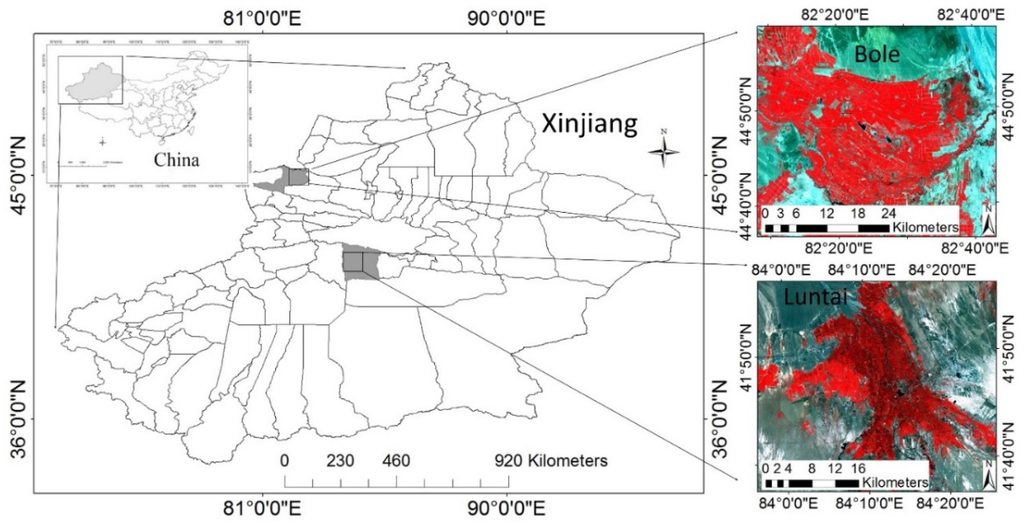
Figure 1.
Locations of the study areas.
3. Method
Time series high spatial resolution remote sensing is the study of the technology for constructing high spatial and temporal resolution remote-sensing data and applications of those data. Usually, the spatial resolution and temporal resolution of the time series high spatial resolution remote-sensing data are higher than 30 m and eight days, respectively. In this study, we combined the HJ CCD, GF-1 WFV, Landsat, and MODIS data to establish a time series of high spatial and temporal resolutions for phenology monitoring and crops mapping. Although the GF-1 WFV data covers the Earth surface every four days and HJ CCD data observe the entire Earth at two-day intervals, there are still gaps greater than eight days in the time series data because of cloud contamination. Zhang et al. [] demonstrated that satellite can monitor the seasonal growth of vegetation successfully if the temporal resolution of satellite data is higher than eight days. To fill the gaps in the time series Normalized Different Vegetation Index (NDVI) data from Landsat, HJ, and GF-1 observations, daily 30 m NDVI data were generated by fusion of MODIS with Landsat, HJ, and GF-1 NDVI data using STDFA.
3.1. Satellite Data
This study collected HJ CCD data sets, GF-1 WFV datasets, and Landsat surface reflectance datasets acquired during clear sky conditions for Bole in 2011 and Luntai in 2013. MODIS surface reflectance data sets were also acquired during clear sky conditions in these two study areas. The number of images from the four kinds of satellite data are shown in Table 1. The Landsat data used in the Bole study area were surface reflectance products, while the other data were Level L1T products.

Table 1.
The number of the four kinds of satellite data used in Bole and Luntai.
| Sensor | Images for Bole | Images for Luntai |
|---|---|---|
| Huanjing satellite charge coupled device (HJ CCD) | 41 | 55 |
| Gaofen satellite no. 1 wide field-of-view camera (GF-1 WFV) | 0 | 18 |
| Landsat Thematic Mapper (TM)/ Operational Land Imager (OLI) | 6 | 10 |
| Moderate Resolution Imaging Spectroradiometer (MODIS) | 154 | 122 |
3.1.1. HJ-1 CCD Data
The HJ satellite constellation consists of two satellites (HJ-1-A and HJ-1-B) launched on 6 September 2008. Both the HJ-1-A and the HJ-1-B satellites are equipped with two CCD cameras. With the four CCD cameras (Table 2), the HJ satellite constellation can image the entire Earth at two-day intervals, with a spatial resolution of 30 m.
Table 2.
Parameters for HJ satellite constellation CCD sensor and GF-1 satellite WFV sensors.
| Sensor | Band | Bandwidth (nm) | Resolution (m) | Width (km) | Return Cycle (Days) |
|---|---|---|---|---|---|
| HJ CCD | 1 | 430–520 | 30 | 700 | 2 |
| 2 | 520–600 | ||||
| 3 | 630–690 | ||||
| 4 | 760–900 | ||||
| GF-1 WFV | 1 | 430–520 | 16 | 800 | 4 |
| 2 | 520–600 | ||||
| 3 | 630–690 | ||||
| 4 | 760–900 |
3.1.2. GF-1 WFV Data
The GF-1 satellite is the first satellite for the Chinese high-resolution earth observation system of national science and technology major projects. It was launched on 26 April 2013. Two WFV sensors were onboard the GF-1 satellite. It can acquire multispectral images at a resolution of 16 m with four-day intervals (Table 2).
3.2. Data Process for the Reconstruction of Time Series High Spatial Resolution Data
A time series of high spatial resolution datasets were generated by combining HJ CCD, GF-1 WFV, Landsat, and MODIS data. The data process includes seven steps: (1) good data selection; (2) atmospheric correction; (3) vegetation index calculation; (4) geometric correction; (5) sensor calibration; (6) spatial and temporal data fusion; and (7) data smoothing.
The data acquired during clear sky conditions were selected. Since there are no cloud products for Landsat, HJ, and GF-1 satellites, a time series of the good quality data were identified from these high spatial resolution data using the visual-interpretation method. Moreover, images with snow cover were also visually removed. The 500 m daily MODIS surface reflectance products (MOD09GA) acquired during clear sky conditions were selected using the data quality of reflectances.
Then, the selected Landsat, HJ, and GF-1 satellites data were atmospherically corrected using the Fast Line-of-Sight Atmospheric Analysis of Spectral Hypercubes (FLAASH) Atmospheric Correction Model. MOD09GA is a level 2G MODIS products that has been atmospherically corrected, so no additional atmospheric correction was needed for those data. These MODIS images were reprojected from the native sinusoidal projection to a UTM-WGS84 reference system, and were resized to the selected study area. The NDVI was then calculated from the time series of Landsat, HJ, GF-1, and MODIS data.
The geometric corrections of Landsat, HJ, and GF-1 data were conducted in two steps. First, one set of Landsat NDVI data was georeferenced using a second-order polynomial warping approach based on the selection of 53 ground control points (GCPs) from a 1:10,000 topographic map using the nearest neighbor resampling method, with a position error of within 0.51 Landsat pixels. Next, the warped Landsat NDVI data was used as a reference image in the geometric corrections of other data. The geometric corrections of other data were conducted using the automatic registration module. This module can select GCPs automatically. Then, these automatically-selected GCPs were checked manually to determine whether they were real GCPs. Wrong GCPs were replaced using GCPs selected manually. The 16 m GF-1 data were resized to 30 m with the pixel aggregate resampling method before the geometric corrections. The MODIS data were georeferenced by a second-order polynomial warping approach based on the selection of 43 GCPs on 500 m Landsat images, with a nearest neighbor resampling method in which the position error was within 0.69 500 m Landsat pixels. The 500 m Landsat images were resized from georeferenced Landsat images using the pixel aggregate resampling method.
Systematic biases were corrected in the NDVI time series from MODIS, Landsat, HJ, and GF-1 observations because these sensor systems have differences in orbit parameters, bandwidth, acquisition time, and spectral response function. Several studies had addressed the problem of sensor difference using linear sensor-adjustment method [,]. However, because the difference between the reflectance of vegetation and non-vegetation in HJ data is much smaller than that of Landsat satellites, a large error occurs in using linear sensor-adjustment methods. In this case, we calibrated the sensor differences one-by-one according to land cover types. The sensor calibration process includes three steps. First, vegetation and non-vegetation were classified using a threshold method for NDVI data. Pixels with NDVI greater than a dynamic threshold were classified as vegetation, while other pixels were classified as non-vegetation. The dynamic threshold value was calculated using regions of interest (ROIs) selected by the visual-interpretation method. Second, linear sensor-adjustment model of vegetation and non-vegetation land cover types were built using the images acquired at the same date, respectively. Landsat-HJ NDVI image pairs acquired on 22 April 2011 in Bole and 19 August 2013 in Luntai were used to build those models for the calibration of Landsat data, respectively. The GF-HJ NDVI image pair acquired on 7 October 2013 in Luntai was used to build the sensor-adjustment model for the calibration of GF-1 data. Finally, these models were used to calibrate all the Landsat and GF-1 data, due to the number of HJ data is higher than the number of Landsat and GF-1 data.
To fill the temporal gaps, the STDFA was used to fuse MODIS with Landsat, HJ, and GF-1 NDVI data using the following formula []:
where and are the fine-resolution reflectances or NDVI of pixels at location (x,y) from time t0 to tk; and are the mean reflectances or NDVI of land cover class c from time t0 to tk which can be calculated using the Ordinary Least Squares technique according linear mixing model []:
where is the residual error term; is the fractional cover of class c in coarse pixel at location (x,y); is the coarse spatial reflectance at time t; and M is the number of land cover types. By inputting two medium-resolution data and time-series MODIS data, time series synthetic medium-resolution data can be generated by STDFA. One medium-resolution data is used for the base image. The other medium-resolution data is used for land cover mapping. To generate synthetic medium-resolution data from time t1 to tn, one actual medium-resolution data with the shortest date interval to this period were used as the base image. The medium-resolution data with the second shortest date interval to this period was selected as another set of medium-resolution data. MODIS data acquired from time t1 to tn were used as the time series MODIS data. Due to this, data fusion is more suitable to generate time series of NDVI data than reflectances [,], daily 30 m NDVI data were generated by fusion MODIS with Landsat, HJ, and GF-1 NDVI data using STDFA. Finally, the time series of high spatial resolution NDVI data sets at each pixel were smoothed using a Savitzky–Golay filter.
3.3. Phenology Detection
Land surface phenology (LPS) [] is defined according to vegetation seasonal growing cycles recorded in time series satellite data. A seasonal cycle of vegetation growth includes a greenup phase, a maturity phase, a senescent phase, and a dormant phase []. Those four phases can be characterized using their start dates. The onset date of greenness increase (OGI) was called greenup onset. The onset date of greenness maximum was called maturity onset. The onset date of greenness decrease was called senescence onset (OGD). The onset date of greenness minimum was called dormancy onset.
To identify the phenology, a Hybrid Piecewise Logistic Model (HPLM) algorithm was used to describe the temporal NDVI data using the following formula []:
where t is time in the day of the year (DOY), a is related to the vegetation growth time, b is associated with the rate of plant leaf development, c is the amplitude of NDVI variation, d is a vegetation stress factor, and NDVIb is the background NDVI value. This model can be applied to detect seasonal vegetation growth successfully, using AVHRR data [,] and MODIS data [,,,].
The vegetation greenup phase and senescence phase were separated using the first derivative value of time series NDVI curve. The first derivative curve shifted from positive to negative was considered the peak of a vegetation seasonal growing cycle. The day before the peak date was considered the greenup phase while the day after the peak date was considered the greenness decrease phase. Then, HPLM algorithm was applied for these two stages, respectively. Since the clouds were masked and snow-covered data were not used, the minimum value in these two stages was used as the background NDVI value. The data earlier than the date of NDVIb were set to the NDVIb value in the greenup phase. The data later than the date of NDVIb were set to the NDVIb value in the greenness decrease phase. The OGI and OGD of the land cover types in Bole and Luntai were calculated using the rate of change in the simulated curves. The date with the maximum first derivative curve in each greenup phase is set to OGI. The date with the minimum first derivative curve in each senescence phase is set to OGD.
Table 3.
The crop calendars of the main crops in Bole and Luntai.
| (a) Cop Calendars in Luntai | ||||||||||||
| Crop | January | February | March | April | May | June | July | August | September | October | November | December |
| Winter wheat | Seeding | Elongating | Earing | Mature | Sowing | Seeding | ||||||
| Cotton | Sowing | Seeding | Bud | Blooming | Mature | |||||||
| Summer corn | Sowing | Seeding | Tasseling | Mature | ||||||||
| (b) Cop Calendars in Bole | ||||||||||||
| Crop | January | February | March | April | May | June | July | August | September | October | November | December |
| Cotton | Sowing | Seeding | Bud | Blooming | Mature | |||||||
| Spring wheat | Sowing | Seeding | Earing | Mature | ||||||||
| Corn | Sowing | Seeding | Seeding | Tasseling | Mature | |||||||
3.4. Crop Mapping
Due to the spectral characteristics of different vegetation are very similar, distinguishing different types of vegetation using multispectral images is quite difficult. However, the crop calendars of the main crops in Bole and Luntai are different (Table 3), allowing us to take advantage of crop phenology information to map crops. Crops in Bole and Luntai were mapped using the phenology information by three steps. First, the vegetation area was extracted using the threshold method. In time series NDVI data, pixels with NDVI greater than 0.2 for a month were classified as vegetation. Other pixels were classified as non-vegetation. Then, the planting patterns for all pixels were extracted according to the number of peaks in the time series NDVI data. According to the ecosystem rules, span between peaks for forest, shrubland or grassland and crops should be longer than four months, two months, and 1.5 months, respectively [], and the land cover types in Luntai and Bole are crops and forest. Thus, pixels with two successive peaks (the time between two peaks being longer than one and a half months) were classified as wheat-corn while the planting patterns of other pixels were set to one crop. Finally, pixels with one-crop planting patterns were classified as tree, cotton, and summer corn, using the maximum likelihood method with two thirds of the field survey data as ROIs for OGI and OGD data.
3.5. Validation
3.5.1. Evaluation of Gap Filling Results
Synthetic NDVI data generated using STDFA methods were evaluated using either HJ NDVI or GF NDVI on the same day. The Synthetic NDVI data in Luntai were evaluated using HJ NDVI on 26 April and GF NDVI on 14 July 2013. Synthetic NDVI data on 26 April 2013 were generated by inputting HJ NDVI data acquired on 22 April 2013 and 7 May 2013 and MODIS NDVI data acquired on 22 and 26 April 2013. Synthetic NDVI data on 14 July 2013 were generated by inputting GF NDVI data acquired on 10 and 18 July 2013 and MODIS NDVI data acquired on 10 and 14 July 2013. The evaluation was performed using parameters of correlation coefficient (r), variance (Var), mean absolute difference (MAD), bias, and root mean square error (RMSE).
3.5.2. Quality Evaluation of Time Series NDVI Data
The quality of time series NDVI data has an important influence on the extraction of phenology and crop mapping. According to the method proposed by Zhang [] and Zema [], the data quality was evaluated using both the proportion of good observations (PGQ) and the model performance index in the time series NDVI data. These two parameters were analyzed for various land cover types and sensors. The land cover types were mapped using the method described in the Section 3.4.
The number of good quality observations in time series NDVI data reflects to a great extent the reliability of detecting the vegetable phenology and mapping crops. As the dormant phase provided no information about vegetation seasonal dynamics, only NDVI data during the vegetation growing season were used in the calculation of PGQ. Since the temporal NDVI trajectory could be well reconstructed with a good NDVI observation within an eight-day period [], a good NDVI observation was counted if there was one good observation within the eight-day windows centered on the date of a scene image. PGQ during a vegetable growing season was calculated as follows:
where Pgq is the proportion of good observations, T is the total number of images during a vegetable growing season, and Ngq is the total number of good quality observations.
Model performance was evaluated using the satellite recorded values with good quality during a vegetation growing season. Several indexes, such as coefficient of determination (R2), coefficient of efficiency (E), modified E (E1), Root Mean Square Error (RMSE), and Coefficient of Residual Mass (CRM), were calculated to quantitatively evaluate the performance of HLPS. Those indexes were defined as follows:
where n is the number of NDVI with good quality, pi is the HPLM simulated NDVI values, oi is the NDVI value with good quality, and is the mean value of oi. This method was widely used to evaluate the performance of different models [,]. According to the work of van Liew and Garbrecht [], E values greater than or equal to 0.75 indicates the observed value can be modeled very well, E values between 0.75 and 0.36 indicates the observed value can be satisfactorily modeled, and E values lower than 0.36 means the modeled value is not reliable.
3.5.3. Verification of Extracted Phenology with Crop Calendars
Since there are no field-measured phenology data, it is impossible to verify the extracted phenology exactly. However, the crop calendars can provide some information about the crop phenology, although it is not accurate to the day. Thus, the crop calendars in Bole and Luntai were used to evaluate the results of phenology extracted by HPLM. If the extracted phenology is consistent with the crop calendars, then the HPLM-simulated phenology is credible.
3.5.4. Verification of Crop Mapping Result with Field Data
There were 525 and 862 plots of field survey data of Bole in 2011 and Luntai in 2013. Two thirds of the field survey data were used as ROIs in the mapping of crops, while other data were used to verify the accuracy of crop mapping. These field-survey data were randomly selected and covered the main land-cover types of each study area. Then, the borders were surveyed using a global position system (GPS). The land-use properties of all plots were obtained through field investigation.
4. Results
4.1. Calibrations of NDVI from Different Sensors
Sixteen Landsat NDVI and 18 GF-1 NDVI data sets were calibrated to HJ NDVI data. After sensor calibration, the sensor differences among these three sensor data were significantly reduced. Table 4 shows the NDVI statistics of vegetation from HJ and GF-1 data acquired on 19 August 2013 in Luntai, and Landsat and HJ data acquired on 7 October 2013 in Luntai. The mean and standard deviation (Stdev) value of vegetation NDVI of HJ, Landsat, and GF-1 WFV sensor showed a large difference before sensor adjustment. After calibration, the mean and Stdev value of those sensors were very close. Figure 2a shows the scatter plots between HJ NDVI and Landsat NDVI and between HJ NDVI and GF-1 WFV NDVI data before sensor calibrations. A large difference in their NDVI data is evident, where the samples were deviated from the 1:1 line. The difference between GF-1 WFV NDVI data and HJ NDVI data is much smaller than the difference between Landsat and HJ NDVI data. After sensor calibration (Figure 2b), the difference was significantly reduced, where most of the samples were distributed along the 1:1 lines.
Table 4.
Normalized Different Vegetation Index (NDVI) statistics of vegetation of each sensors in Luntai.
| Image Date | Sensor | NDVI of Vegetation | |
|---|---|---|---|
| Mean | Standard Deviation (Stdev) | ||
| 7 October 2013 | HJ | 0.3589 | 0.0923 |
| GF | 0.4163 | 0.1083 | |
| Adjusted GF | 0.3587 | 0.0973 | |
| 19 August 2013 | HJ | 0.5477 | 0.1646 |
| Landsat | 0.6072 | 0.2732 | |
| Adjusted Landsat | 0.5525 | 0.1657 | |
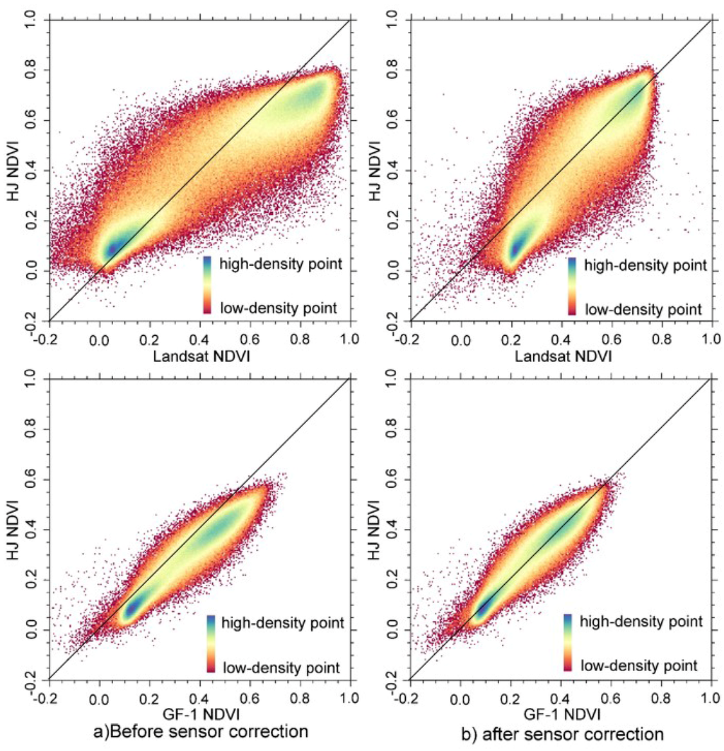
Figure 2.
The scatter plot comparisons of Landsat Normalized Different Vegetation Index (NDVI) data, Gaofen satellite no. 1 wide field-of-view camera (GF-1 WFV) NDVI, and Huanjing satellite (HJ) NDVI data (a) before and (b) after sensor calibration.
4.2. Gap Filling NDVI Time Series and Evaluation
By fusing daily MODIS data with HJ CCD, Landsat and GF-1 WFV data using STDFA, daily 30 m synthetic NDVI data were generated. There were 54 synthetic DNVI data in Luntai and 69 synthetic DNVI data in Bole. Figure 3 shows a synthetic HJ NDVI for 26 April 2013 and a synthetic GF NDVI for 14 July 2013. Through visual-interpretation method, we can find that the synthetic NDVI are very similar with the actual NDVI. Both the synthetic and actual NDVI have a higher spatial resolution that the MODIS NDVI. The evaluation of these two synthetic NDVI data using HJ NDVI and GF NDVI shows that the r value is greater than 0.97 and RMSE error is less than 0.04 (Table 5). It shows that the synthetic NDVI using the STDFA method is very similar to actual NDVI data. Consistent with the results of Wu et al. [], the STDFA method showed a better performance in homogeneous land cover types (desert and large area farmland) than in heterogeneity plots (small area woodland). Consistent with the results of Wu et al. [], the STDFA method showed a better performance in the GF-MODIS fusion than in the HJ-MODIS fusion, because the GF-1 data have a higher quality than the HJ CCD data. The geometric registration error also showed an important influence in the performance of STDFA. Due to the geometric registration error of the lower right part of GF-1 WFV data being larger than in the upper left part, a smaller difference between the synthetic and actual GF-1 WFV data (14 July 2013) was obtained by the STDFA in the upper left part.
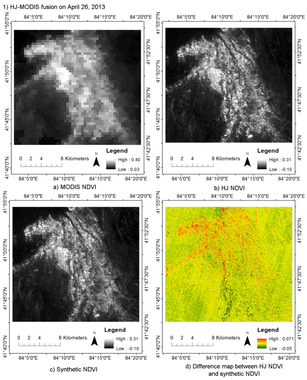
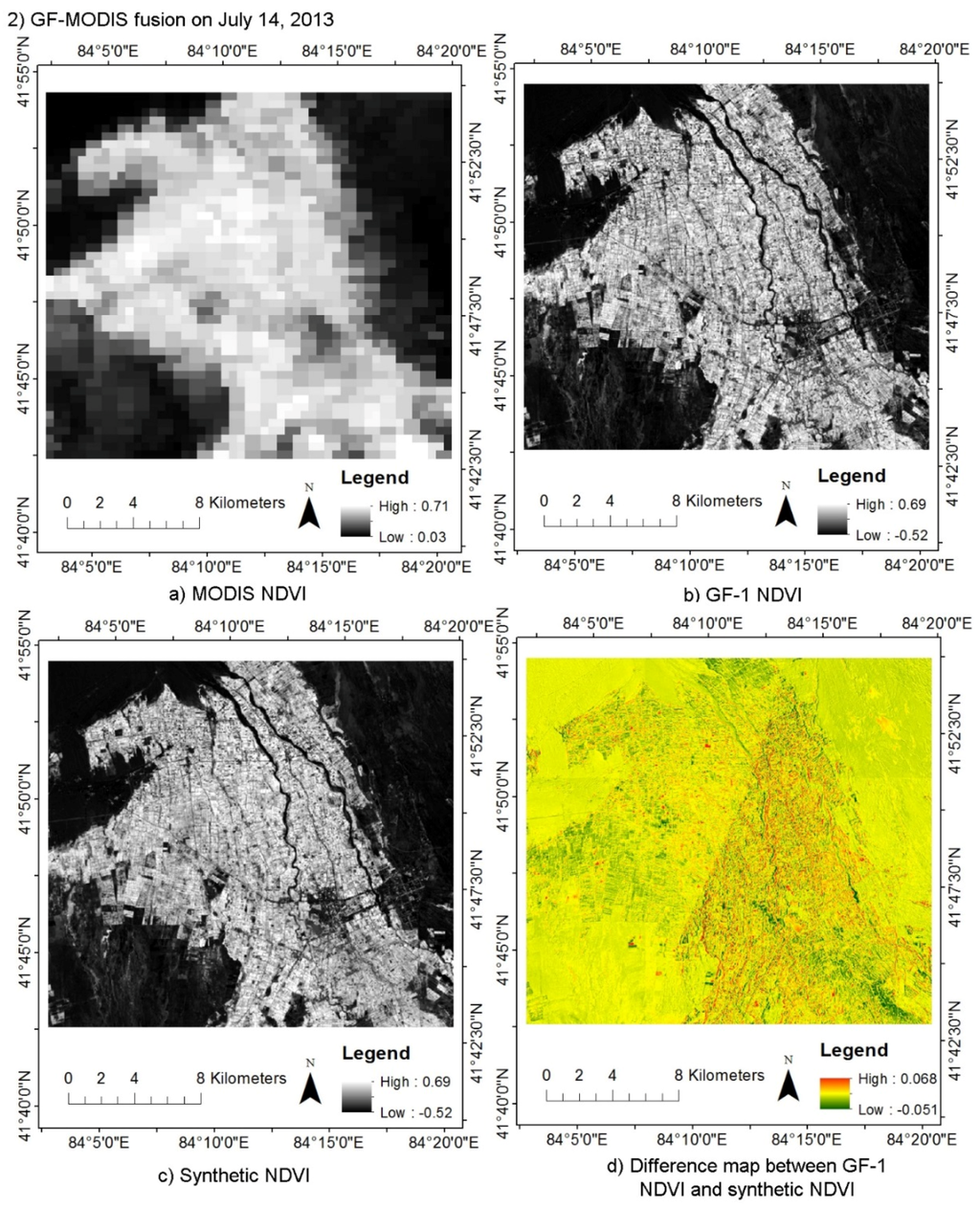
Figure 3.
Comparison of Moderate Resolution Imaging Spectroradiometer (MODIS) NDVI, HJ NDVI, GF-1 NDVI, and synthetic NDVI generated by the Spatial and Temporal Data Fusion Approach (STDFA): (a) MODIS NDVI; (b) HJ NDVI; (c) Synthetic NDVI; and (d) difference map between HJ NDVI and synthetic NDVI in (1) HJ-MODIS fusion result comparison on April 26, 2013; (a) MODIS NDVI; (b) GF-1 NDVI; (c) Synthetic NDVI; and (d) difference map between GF-1 NDVI and synthetic NDVI in (2) GF-MODIS fusion result comparison on 14 July 2013.
Table 5.
Results of the correlation analysis between synthetic and actual HJ, GF NDVI data.
| Correlation Coefficient (r) | Variance (Var) | Mean Absolute Difference (MAD) | Root Mean Square Error (RMSE) | Bias | |
|---|---|---|---|---|---|
| HJ-MODIS Fusion | 0.9702 | 0.0003 | 0.0121 | 0.0230 | −0.0162 |
| GF-MODIS Fusion | 0.9813 | 0.0016 | 0.0257 | 0.0464 | −0.0243 |
4.3. Assessment of the Reconstructed Time Series High Spatial Data
Two time series of 30 m NDVI data sets were reconstructed. There were 131 NDVI data sets for Luntai, including four Landsat NDVI, 20 GF-1 NDVI, 53 HJ NDVI, and 54 synthetic NDVI. There were 117 NDVI data sets for Bole, including six Landsat NDVI, 42 HJ NDVI, and 69 synthetic NDVI. The Landsat NDVI and GF-1 NDVI acquired for the same day as HJ NDVI were not used.
To assess the quality of reconstructed time series of 30 m NDVI data, the PGQ and the model performance index were calculated. Since only images acquired in clear sky conditions were used, the PGQs for all pixels in Bole and Luntai are the same. To show the ability of each sensor to reconstruct time series high spatial data, the PGQs were calculated for varying sensor types. Table 6 shows that the PGQs of HJ and GF-1 satellites are far higher than those of Landsat, because the return cycles of HJ and GF-1 satellites are much higher that of Landsat.
Table 6.
Proportion of good observations (PGQ) of each satellite.
| Study Area | Landsat | GF-1 | HJ | Landsat + GF-1 + HJ |
|---|---|---|---|---|
| Luntai | 0.1832 | 0.8592 * | 0.9695 | 0.9847 |
| Bole | 0.3162 | 0.0000 | 0.9829 | 0.9829 |
* The GF-1 satellite acquired image after 2 July 2013 in Luntai. Only the data after 2 July 2013 were used to calculate the PGQ for GF-1 satellite.
Quantitative evaluation of the model performance showed that the HPLM approach can simulate time series NDVI very well with R2 ranged from 0.635 to 0.952 in Luntai and 0.719 to 0.991 in Bole, respectively (Figure 4). The RMSE in Luntai and Bole is ranged from 0 to 0.096 and 0 to 0.111, respectively. Most of pixels have an E value higher than 0.36 (Figure 5). It showed that most of the simulated values were reliable. The CRM in Luntai and Bole ranged from −0.054 to 0.187 and −0.117 to 0.002, respectively.
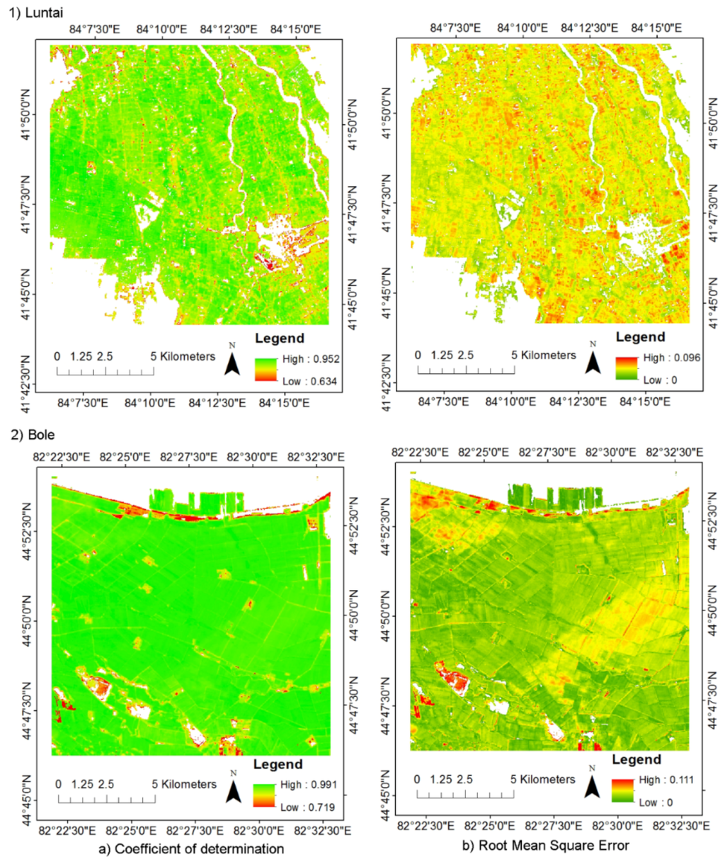
Figure 4.
Results of model performance quantitative evaluation: (a) coefficient of determination (R2) in (1) Luntai and (2) Bole; and (b) root mean square error (RMSE) in (1) Luntai and (2) Bole.
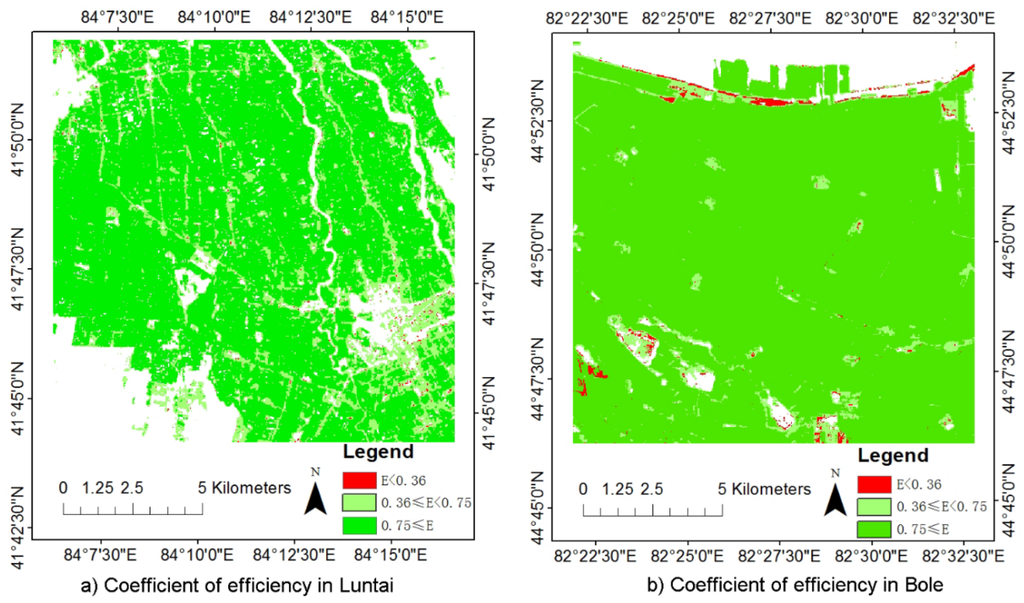
Figure 5.
Coefficient of efficiency (E) values in (a) Luntai and (b) Bole.
Thus, a higher PGQ index and model performance index showed a good quality of reconstructed time series of 30 m NDVI data, both for Bole and for Luntai, indicating these data can be used in phenological extraction and crop mapping.
4.4. Phenology from Reconstructed NDVI Time Series and Evaluation
Figure 6 shows the simulated mean NDVI phenology of the field survey plots in different land cover types. It shows that different land cover types have different phenological curves. The OGI of tree is earlier than that of cotton and corn. The OGD of tree is later than that of cotton and corn. The OGD of cotton is later than that of corn. Figure 7 shows the calculated OGI and OGD in Bole and Luntai. Difference land cover types have difference OGI and OGD distribution. Table 7 shows the calculated OGI and OGD for the land cover types. Comparing Table 3 and Table 7, we can see that the simulated phenology of each land cover type fit well with the crop calendars of the main crops in Bole and Luntai.
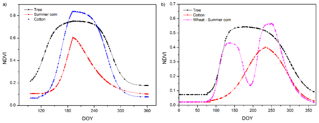
Figure 6.
Simulated phenology for all land cover types in (a) Bole and (b) Luntai.
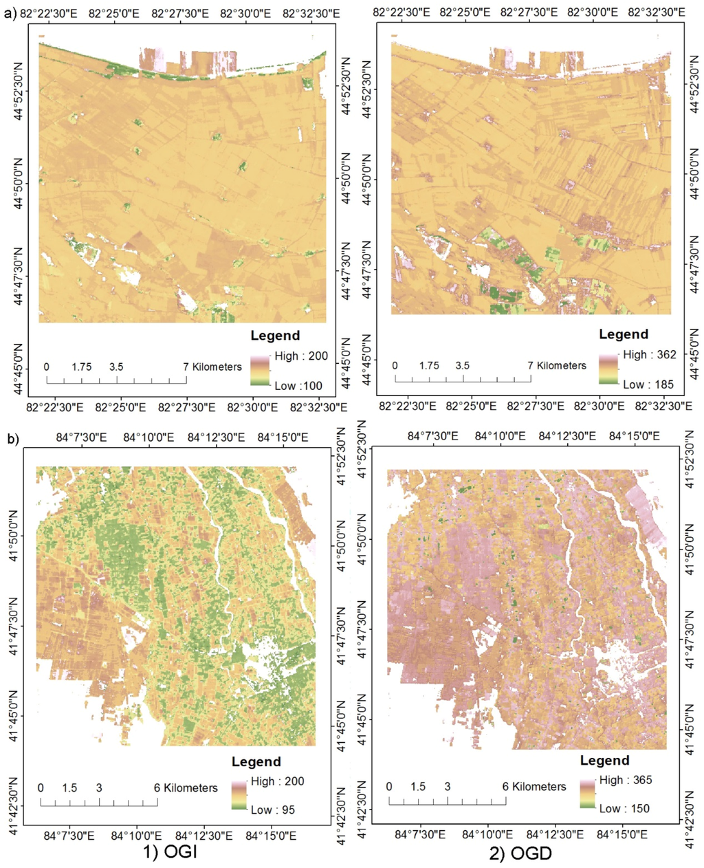
Figure 7.
Calculated onset date of greenness increase (OGI) and greenness decrease (OGD) in (a) Bole and (b) Luntai.
Table 7.
The onset date of greenness increase (OGI) and greenness decrease (OGD) of each land use types in Luntai and Bole.
| Planting Patterns | Land Use | Luntai | Bole | ||
|---|---|---|---|---|---|
| OGI (DOY) | OGD (DOY) | OGI (DOY) | OGD (DOY) | ||
| One crop | Tree | 115 | 308 | 109 | 298 |
| Cotton | 161 | 276 | 163 | 275 | |
| Summer corn | 174 | 230 | |||
| Wheat-Summer corn | Wheat | 111 | 177 | ||
| Summer corn | 204 | 283 | |||
4.5. Crop-Mapping from Phenology and Validation
Figure 8 shows the land cover types in Bole and Luntai mapped using phenology information extracted from the reconstructed time series of 30 m NDVI data. The results indicate that the cotton and corn plots were well classified. Moreover, the trees on the side of road were also extracted. Table 8 shows the accuracy evaluation using field survey data for Bole and Luntai. The results show that land cover types were mapped with an accuracy of higher than 90%.
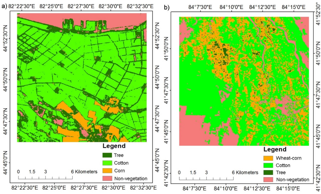
Figure 8.
Land cover types in (a) Bole and (b) Luntai.
Table 8.
Accuracy evaluations of (1) Luntai and (2) Bole.
| (1) Luntai: Overall Accuracy = 91.03%; Kappa Coefficient = 0.8483 | |||||
| Class | Reference Data | Producer Accuracy (%) | User Accuracy (%) | ||
| Wheat-corn | Cotton | Tree | |||
| Wheat-corn | 87.32 | 0 | 0 | 87.32 | 100 |
| Cotton | 1.17 | 100.00 | 28.05 | 100 | 92.71 |
| Tree | 11.51 | 0 | 71.95 | 71.95 | 53.54 |
| (2) Bole: Overall Accuracy = 95.08%; Kappa Coefficient = 0.9235 | |||||
| Class | Reference Data | Producer Accuracy (%) | User Accuracy (%) | ||
| Tree | Cotton | Corn | |||
| Tree | 98.75 | 2.60 | 8.98 | 98.75 | 80.49 |
| Cotton | 0.51 | 97.15 | 0.88 | 97.15 | 99.54 |
| Corn | 0.74 | 0.25 | 90.14 | 90.14 | 98.7 |
5. Discussion
5.1. Useful Data Comparison
To show the good data acquisition ability of all sensors, the proportion of days of good data for all sensors were calculated and compared. Table 9 shows the proportion of days of good data for all sensors for Luntai. It demonstrates that both the proportion of days with good data in HJ and GF was much higher than that for Landsat. By combining HJ, GF, Landsat, and MODIS data, the reconstructed time series of high spatial resolution data present the highest proportion of days with good data.
Table 9.
The proportion of days with good data in each sensor in Luntai.
| Sensor | HJ | GF | MODIS | OLI | HJ + GF | Fusion Data |
|---|---|---|---|---|---|---|
| Useful data number | 55 | 18 | 139 | 10 | 70 | 162 |
| The proportion of days of good data (%) | 0.15 | 0.10 | 0.38 | 0.04 | 0.19 | 0.44 |
| Max gap (day) | 34 | 36 | 14 | 80 | 34 | 11 |
| Mean gap (day) | 8 | 6.35 | 2.64 | 32 | 4.9 | 2.26 |
5.2. Comparison with MODIS
Figure 9 shows the phenology for all land cover types extracted from actual daily 500 m MODIS NDVI data. Comparing Figure 6 and Figure 9, their NDVI phenological trajectories were very similar. The OGI and OGD calculated from time series 500 m MODIS NDVI data in Bole and Luntai (Table 10) were also fitted well with the crop calendars of the main crops (Table 3) and the OGI and OGD calculated from time series of the high spatial resolution data (Table 7). However, the largest difference of OGI and OGD between MODIS NDVI and 30 m NDVI detections was 12 days in Luntai and three days in Bole.
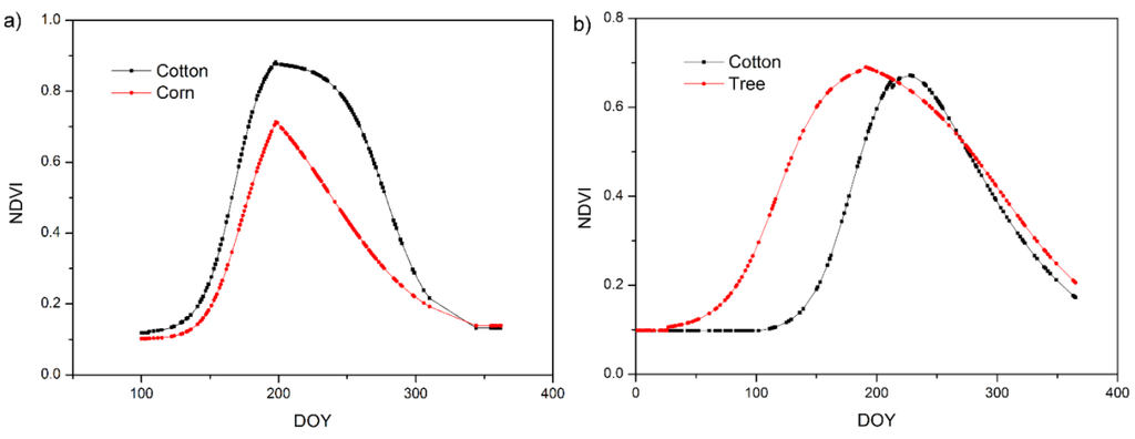
Figure 9.
Phenology for different land cover types extracted from actual MODIS NDVI data in (a) Bole and (b) Luntai.
Table 10.
The OGI and OGD for each land use type extracted by MODIS NDVI data in Luntai and Bole.
| Land Use | Luntai | Bole | ||
|---|---|---|---|---|
| OGI (DOY) | OGD (DOY) | OGI (DOY) | OGD (DOY) | |
| Tree | 116 | 296 | ||
| Cotton | 158 | 278 | 162 | 277 |
| Summer corn | 172 | 227 | ||
Due to the high spatial resolution, the time series data has two advantages. First, much information can be directly obtained through visual interpretation of the time series high spatial resolution data, such as the land cover types, the OGI and OGD of each land cover type, and data quality information (clouds or snow cover). Second, land cover types in most pixels are pure, allowing more sophisticated classification. For example, roadside trees in Bole and wheat-corn in small plots in Luntai can be well classified. However, the disadvantage of using those data is the large data-processing workload, especially using HJ and GF-1 data, including cloud masking and atmospheric and geometric correction. Due to the high spatial resolution, the data storage space is very large. For example, the data storage space for a 480 × 480 30 m area in Bole is more than 300 GB. In addition, both the HJ and GF-1 data are non-standardized data, where the radiation accuracy, clarity, and signal to noise ratio of HJ CCD data are lower than Landsat TM data []. Overall, time series high spatial resolution data are more suitable for small area detailed phenology extraction.
In contrast to time series high spatial resolution data, time series MODIS data are more suitable for phenology extraction in large scale areas. Due to the low spatial resolution, the data storage space for MODIS data is much smaller. However, when the size of land objects are smaller, a MODIS pixel often represents a mixture of different land cover types, making it difficult to classify high spatial resolution land-cover types and to extract phenology. For example, roadside trees in Bole and wheat-corn in small plots in Luntai cannot be classified using time series 500 m MODIS NDVI data. Further, obtaining land cover information from the visual information in the low spatial resolution data is difficult.
5.3. Comparison with Other Mapping Methods
To demonstrate the advantage of the reconstructed time series high spatial resolution data in the application of crop mapping, crops were mapped using multi-temporal Landsat NDVI data using the maximum likelihood method with the same AOIs used in the crop classification with time series high spatial resolution data. Table 11 shows the Landsat data used in the mapping of crops in Bole and Luntai. The mapping accuracy was evaluated using field survey data in Bole and Luntai (Table 12). A comparison between Table 8 and Table 12 shows the crop maps classified using the reconstructed time series high spatial resolution data have a higher accuracy than those classified using the time series Landsat NDVI data. The overall accuracy of crop maps classified using the reconstructed time series high spatial resolution data are 0.91 in Luntai and 0.95 in Bole, which is 0.028 and 0.046 higher than those obtained by using multi-temporal Landsat NDVI data. Thus, the reconstructed time series high spatial resolution data can be used for detailed crop mapping.
Table 11.
Landsat data using in the classification of crops in Luntai and Bole.
| Bole | Luntai | ||||
|---|---|---|---|---|---|
| Sensor | Path/Row | Acquisition Date | Sensor | Path/Row | Acquisition Date |
| Landsat-5 TM | 146/29 | 6/4/2011 | Landsat-8 OLI | 144/31 | 13/4/2013 |
| 22/4/2013 | 15/5/2013 | ||||
| 24/5/2013 | 31/5/2013 | ||||
| 11/7/2013 | 19/8/2013 | ||||
| 27/7/2013 | 4/9/2013 | ||||
| 13/9/2013 | 6/10/2013 | ||||
| 22/10/2013 | |||||
Table 12.
Accuracy evaluations of (1) Luntai and (2) Bole.
| (1) Luntai: Overall Accuracy = 88.21%; Kappa Coefficient = 0.8042 | |||||
| Class | Reference Data | Producer Accuracy (%) | User Accuracy (%) | ||
| Wheat-corn | Cotton | Tree | |||
| Wheat-corn | 78.90 | 0.93 | 7.55 | 78.90 | 97.83 |
| Cotton | 0.17 | 99.07 | 0.00 | 99.07 | 99.79 |
| Tree | 20.93 | 0.00 | 92.45 | 92.45 | 36.93 |
| (2) Bole: Overall Accuracy = 90.49%; Kappa Coefficient = 0.8170 | |||||
| Class | Reference Data | Producer Accuracy (%) | User Accuracy (%) | ||
| Tree | Cotton | Corn | |||
| Tree | 68.75 | 7.88 | 1.44 | 68.75 | 61.81 |
| Cotton | 28.76 | 92.05 | 0.11 | 92.05 | 94.16 |
| Corn | 2.50 | 0.06 | 98.45 | 98.45 | 98.37 |
5.4. Limitations
Comparing with time series MODIS data and multi-temporal Landsat data, the reconstructed daily 30 m data showed a better performance in phenology extracting and crop mapping. However, it also has limitations. First, as mentioned in Section 5.2, it requires a lot of data processing work. Second, although the STDFA can generate synthetic 30 m data with a high accuracy, the simulated 30 m data also showed a small difference with the actual image. This problem can be addressed by launching new satellites to acquire real high spatial and temporal resolution data. Third, the environmental factors (e.g., precipitation, temperature, soil type, soil moisture) or management practices (e.g., sowing date, fertilization) were not considered in the phenology monitoring and crops mapping. This should be an important work for the future studies.
6. Conclusions
This study developed a data process framework for reconstructing time series high spatial resolution remote-sensing data and applied it in phenology monitoring and crop mapping. The approaches were demonstrated using data in two study areas located at Xinjiang, China. The results show that the STDFA method was able to reconstruct the time series high spatial resolution remote-sensing data from HJ CCD, GF-1 WFV, Landsat, and MODIS data. The time series high spatial resolution remote-sensing data were able to extract vegetation phenology reliably, which produced much detailed vegetation phenology than time series MODIS NDVI data did. Finally, the time series high spatial resolution remote-sensing data were capable of mapping crops types, which produced a higher accuracy than that from multi-temporal Landsat NDVI data.
Acknowledgments
This work was supported by the National Natural Science Foundation of China (41301390), the National Science and Technology Major Project (2014AA06A511), the Major State Basic Research Development Program of China (2013CB733405, 2010CB950603), and the National Science and Technology Major Project of China. The funders had no role in choosing the study design, in the collection, analysis, and interpretation of the data, in the writing of the report, or in the decision to submit the article for publication.
Author Contributions
Mingquan Wu, Wenjiang Huang, Zheng Niu and Changyao Wang conceived and designed the experiments. Mingquan Wu performed the experiments and the manuscript draft. Xiaoyang Zhang directed the experiments. Xiaoyang Zhang, Wenjiang Huang, Zheng Niu, Changyao Wang, Wang Li and Pengyu Hao revised the manuscript draft. All authors read and approved the final version.
Conflicts of Interest
The authors declare no conflict of interest.
References
- Fensholt, R.; Anyamba, A.; Huber, S.; Proud, S.R.; Tucker, C.J.; Small, J.; Pak, E.; Rasmussen, M.O.; Sandholt, I.; Shisanya, C. Analysing the advantages of high temporal resolution geostationary MSG SEVIRI data compared to Polar Operational Environmental Satellite data for land surface monitoring in Africa. Int. J. Appl. Earth Observ. Geoinf. 2011, 13, 721–729. [Google Scholar] [CrossRef]
- Maisongrande, P.; Duchemin, B.; Dedieu, G. VEGETATION/SPOT: An operational mission for the Earth monitoring; presentation of new standard products. Int. J. Remote Sens. 2004, 25, 9–14. [Google Scholar] [CrossRef]
- Politi, E.; Cutler, M.E.J.; Rowan, J.S. Using the NOAA Advanced Very High Resolution Radiometer to characterise temporal and spatial trends in water temperature of large European lakes. Remote Sens. Environ. 2012, 126, 1–11. [Google Scholar] [CrossRef]
- Salomonson, V.V.; Barnes, W.L.; Maymon, P.W.; Montgomery, H.E.; Ostrow, H. MODIS—Advanced facility instrument for studies of the earth as a system. IEEE Trans. Geosci. Remote Sens. 1989, 27, 145–153. [Google Scholar] [CrossRef]
- Xue, C.J.; Song, W.J.; Qin, L.J.; Dong, Q.; Wen, X.Y. A spatiotemporal mining framework for abnormal association patterns in marine environments with a time series of remote sensing images. Int. J. Appl. Earth Observ. Geoinf. 2015, 38, 105–114. [Google Scholar] [CrossRef]
- Zhang, J.H.; Feng, L.L.; Yao, F.M. Improved maize cultivated area estimation over a large scale combining MODIS–EVI time series data and crop phenological information. ISPRS J. Photogramm. Remote Sens. 2014, 94, 102–113. [Google Scholar] [CrossRef]
- Zuo, L.J.; Wang, X.; Liu, F.; Yi, L. Spatial exploration of multiple cropping efficiency in China based on time series remote sensing data and econometric model. J. Integr. Agric. 2013, 12, 903–913. [Google Scholar] [CrossRef]
- Chen, L.F.; Jin, Z.Y.; Michishita, R.; Cai, J.; Yue, T.X.; Chen, B.; Xu, B. Dynamic monitoring of wetland cover changes using time-series remote sensing imagery. Ecol. Inf. 2014, 24, 17–26. [Google Scholar] [CrossRef]
- Eckert, S.; Husler, F.; Liniger, H.; Hodel, E. Trend analysis of MODIS NDVI time series for detecting land degradation and regeneration in Mongolia. J. Arid Environ. 2015, 113, 16–28. [Google Scholar] [CrossRef]
- Estel, S.; Kuemmerle, T.; Alcantara, C.; Levers, C.; Prishchepov, A.; Hostert, P. Mapping farmland abandonment and recultivation across Europe using MODIS NDVI time series. Remote Sens. Environ. 2015, 163, 312–325. [Google Scholar] [CrossRef]
- Palmer, S.C.J.; Odermatt, D.; Hunter, P.D.; Brockmann, C.; Presing, M.; Balzter, H.; Toth, V.R. Satellite remote sensing of phytoplankton phenology in Lake Balaton using 10 years of MERIS observations. Remote Sens. Environ. 2015, 158, 441–452. [Google Scholar] [CrossRef]
- Zhang, X.Y.; Tan, B.; Yu, Y.Y. Interannual variations and trends in global land surface phenology derived from enhanced vegetation index during 1982–2010. Int. J. Biometeorol. 2014, 58, 547–564. [Google Scholar] [CrossRef] [PubMed]
- Dedieu, J.P.; Lessard-Fontaine, A.; Ravazzani, G.; Cremonese, E.; Shalpykova, G.; Beniston, M. Shifting mountain snow patterns in a changing climate from remote sensing retrieval. Sci. Total Environ. 2014, 493, 1267–1279. [Google Scholar] [CrossRef] [PubMed]
- Mohan, M.; Kandya, A. Impact of urbanization and land-use/land-cover change on diurnal temperature range: A case study of tropical urban airshed of India using remote sensing data. Sci. Total Environ. 2015, 506, 453–465. [Google Scholar] [CrossRef] [PubMed]
- Willis, K.S. Remote sensing change detection for ecological monitoring in United States protected areas. Biol. Conserv. 2015, 182, 233–242. [Google Scholar] [CrossRef]
- Beuchle, R.; Grecchi, R.C.; Shimabukuro, Y.E.; Seliger, R.; Eva, H.D.; Sano, E.; Achard, F. Land cover changes in the Brazilian Cerrado and Caatinga biomes from 1990 to 2010 based on a systematic remote sensing sampling approach. Appl. Geogr. 2015, 58, 116–127. [Google Scholar] [CrossRef]
- Gong, P.; Wang, J.; Yu, L.; Zhao, Y.C.; Zhao, Y.Y.; Liang, L.; Niu, Z.G.; Huang, X.M.; Fu, H.H.; Liu, S.; et al. Finer resolution observation and monitoring of global land cover: First mapping results with Landsat TM and ETM+ data. Int. J. Remote Sens. 2013, 34, 2607–2654. [Google Scholar] [CrossRef]
- Jia, K.; Liang, S.L.; Zhang, N.; Wei, X.Q.; Gu, X.F.; Zhao, X.; Yao, Y.J.; Xie, X.H. Land cover classification of finer resolution remote sensing data integrating temporal features from time series coarser resolution data. ISPRS J. Photogramm. Remote Sens. 2014, 93, 49–55. [Google Scholar] [CrossRef]
- Löw, F.; Fliemann, E.; Abdullaev, I.; Conrad, C.; Lamers, J.P.A. Mapping abandoned agricultural land in Kyzyl-Orda, Kazakhstan using satellite remote sensing. Appl. Geogr. 2015, 62, 377–390. [Google Scholar] [CrossRef]
- He, Y.Q.; Ai, B.; Yao, Y.; Zhong, F.J. Deriving urban dynamic evolution rules from self-adaptive cellular automata with multi-temporal remote sensing images. Int. J. Appl. Earth Observ. Geoinform. 2015, 38, 164–174. [Google Scholar] [CrossRef]
- Isenstein, E.M.; Park, M.H. Assessment of nutrient distributions in Lake Champlain using satellite remote sensing. J. Environ. Sci. China 2014, 26, 1831–1836. [Google Scholar] [CrossRef] [PubMed]
- Luo, J.; Li, X.; Ma, R.; Li, F.; Duan, H.; Hu, W.; Qin, B.; Huang, W. Applying remote sensing techniques to monitonterannual changes of aquatic vegetation in Taihu Lake, China. Ecol. Indic. 2016, 60, 503–513. [Google Scholar]
- Leckie, D.G. Advances in remote-sensing technologies for forest surveys and management. Can. J. For. Res. 1990, 20, 464–483. [Google Scholar] [CrossRef]
- Gao, F.; Masek, J.; Schwaller, M.; Hall, F. On the blending of the Landsat and MODIS surface reflectance: Predicting daily Landsat surface reflectance. IEEE Trans. Geosci. Remote Sens. 2006, 44, 2207–2218. [Google Scholar]
- Hilker, T.; Wulder, M.A.; Coops, N.C.; Linke, J.; McDermid, G.; Masek, J.G.; Gao, F.; White, J.C. A new data fusion model for high spatial- and temporal-resolution mapping of forest disturbance based on Landsat and MODIS. Remote Sens. Environ. 2009, 113, 1613–1627. [Google Scholar] [CrossRef]
- Liu, H.; Weng, Q.H. Enhancing temporal resolution of satellite imagery for public health studies: A case study of West Nile Virus outbreak in Los Angeles in 2007. Remote Sens. Environ. 2012, 117, 57–71. [Google Scholar] [CrossRef]
- Schmidt, M.; Lucas, R.; Bunting, P.; Verbesselt, J.; Armston, J. Multi-resolution time series imagery for forest disturbance and regrowth monitoring in Queensland, Australia. Remote Sens. Environ. 2015, 158, 156–168. [Google Scholar] [CrossRef]
- Walker, J.J.; de Beurs, K.M.; Wynne, R.H.; Gao, F. Evaluation of Landsat and MODIS data fusion products for analysis of dryland forest phenology. Remote Sens. Environ. 2012, 117, 381–393. [Google Scholar] [CrossRef]
- Weng, Q.H.; Fu, P.; Gao, F. Generating daily land surface temperature at Landsat resolution by fusing Landsat and MODIS data. Remote Sens. Environ. 2014, 145, 55–67. [Google Scholar] [CrossRef]
- Zhu, X.L.; Chen, J.; Gao, F.; Chen, X.H.; Masek, J.G. An enhanced spatial and temporal adaptive reflectance fusion model for complex heterogeneous regions. Remote Sens. Environ. 2010, 114, 2610–2623. [Google Scholar] [CrossRef]
- Emelyanova, I.V.; McVicar, T.R.; van Niel, T.G.; Li, L.T.; van Dijk, A. Assessing the accuracy of blending Landsat–MODIS surface reflectances in two landscapes with contrasting spatial and temporal dynamics: A framework for algorithm selection. Remote Sens. Environ. 2013, 133, 193–209. [Google Scholar] [CrossRef]
- Busetto, L.; Meroni, M.; Colombo, R. Combining medium and coarse spatial resolution satellite data to improve the estimation of sub-pixel NDVI time series. Remote Sens. Environ. 2008, 112, 118–131. [Google Scholar] [CrossRef]
- Maselli, F. Definition of spatially variable spectral endmembers by locally calibrated multivariate regression analyses. Remote Sens. Environ. 2001, 75, 29–38. [Google Scholar] [CrossRef]
- Zhukov, B.; Oertel, D.; Lanzl, F.; Reinhackel, G. Unmixing-based multisensor multiresolution image fusion. IEEE Trans. Geosci. Remote Sens. 1999, 37, 1212–1226. [Google Scholar] [CrossRef]
- Wu, M.; Huang, W.; Niu, Z.; Wang, C. Generating Daily Synthetic Landsat Imagery by Combining Landsat and MODIS data. Sensors 2015, 15, 24002–24025. [Google Scholar] [CrossRef] [PubMed]
- Wu, M.Q.; Niu, Z.; Wang, C.Y.; Wu, C.Y.; Wang, L. Use of MODIS and Landsat time series data to generate high-resolution temporal synthetic Landsat data using a spatial and temporal reflectance fusion model. J. Appl. Remote Sens. 2012, 6. [Google Scholar] [CrossRef]
- Wu, M.Q.; Wu, C.Y.; Huang, W.J.; Niu, Z.; Wang, C.Y. High-resolution Leaf Area Index estimation from synthetic Landsat data generated by a spatial and temporal data fusion model. Comput. Electron. Agric. 2015, 115, 1–11. [Google Scholar] [CrossRef]
- Wu, M.Q.; Li, H.; Huang, W.J.; Niu, Z.; Wang, C.Y. Generating daily high spatial land surface temperatures by combining ASTER and MODIS land surface temperature products for environmental process monitoring. Environ. Sci. Process. Impacts 2015, 17, 1396–1404. [Google Scholar] [CrossRef] [PubMed]
- Gevaert, C.M.; Garcia-Haro, F.J. A comparison of STARFM and an unmixing-based algorithm for Landsat and MODIS data fusion. Remote Sens. Environ. 2015, 156, 34–44. [Google Scholar] [CrossRef]
- Wu, M.Q.; Huang, W.J.; Niu, Z.; Wang, C.Y. Combining HJ CCD, GF-1 WFV and MODIS data to generate daily high spatial resolution synthetic data for environmental process monitoring. Int. J. Environ. Res. Public Health 2015, 12, 9920–9937. [Google Scholar] [CrossRef] [PubMed]
- Zhang, X.; Friedl, M.; Schaaf, C. Sensitivity of vegetation phenology detection to the temporal resolution of satellite data. Int. J. Remote Sens. 2009, 30, 2061–2074. [Google Scholar] [CrossRef]
- Settle, J.J.; Drake, N.A. Linear mixing and the estimation of groundcover proportion. Int. J. Remote Sens. 1993, 14, 1159–1177. [Google Scholar] [CrossRef]
- De Beurs, K.M.; Henebry, G.M. Land surface phenology, climatic variation, and institutional change: Analyzing agricultural land cover change in Kazakhstan. Remote Sens. Environ. 2004, 89, 497–509. [Google Scholar] [CrossRef]
- Zhang, X.; Friedl, M.A.; Schaaf, C.B.; Strahler, A.H.; Hodges, J.C.F.; Gao, F.; Reed, B.C.; Huete, A. Monitoring vegetation phenology using MODIS. Remote Sens. Environ. 2003, 84, 471–475. [Google Scholar] [CrossRef]
- Zhang, X.Y. Reconstruction of a complete global time series of daily vegetation index trajectory from long-term AVHRR data. Remote Sens. Environ. 2015, 156, 457–472. [Google Scholar] [CrossRef]
- Julien, Y.; Sobrino, J.A. Global land surface phenology trends from GIMMS database. Int. J. Remote Sens. 2009, 30, 3495–3513. [Google Scholar] [CrossRef]
- Zhang, X.Y.; Tarpley, D.; Sullivan, J.T. Diverse responses of vegetation phenology to a warming climate. Geophys. Res. Lett. 2007, 34. [Google Scholar] [CrossRef]
- Liang, L.A.; Schwartz, M.D.; Fei, S.L. Validating satellite phenology through intensive ground observation and landscape scaling in a mixed seasonal forest. Remote Sens. Environ. 2011, 115, 143–157. [Google Scholar] [CrossRef]
- Zhang, X.Y.; Friedl, M.A.; Schaaf, C.B. Global vegetation phenology from Moderate Resolution Imaging Spectroradiometer (MODIS): Evaluation of global patterns and comparison with in situ measurements. J. Geophys. Res. Biogeosci. 2006, 111. [Google Scholar] [CrossRef]
- Zema, D.A.; Bingner, R.L.; Denisi, P.; Govers, G.; Licciardello, F.; Zimbone, S.M. Evaluation of runoff, peak flow and sediment yield for events simulated by the AnnAGNPS model in a Belgian agricultural watershed. Land Degrad. Dev. 2012, 23, 205–215. [Google Scholar] [CrossRef]
- Chahor, Y.; Casali, J.; Gimenez, R.; Bingner, R.L.; Campo, M.A.; Goni, M. Evaluation of the AnnAGNPS model for predicting runoff and sediment yield in a small mediterranean agricultural watershed in Navarre (Spain). Agric. Water Manag. 2014, 134, 24–37. [Google Scholar] [CrossRef]
- Van Liew, M.W.; Garbrecht, J. Hydrologic simulation of the little washita river experimental watershed using SWAT. J. Am. Water Resour. Assoc. 2003, 39, 413–426. [Google Scholar] [CrossRef]
- Wei, H.W.; Tian, Q.J. Quality evalution and analysis of HJ-1B-CCD images. Remote Sens. Inf. 2012, 207, 31–36. [Google Scholar]
© 2015 by the authors; licensee MDPI, Basel, Switzerland. This article is an open access article distributed under the terms and conditions of the Creative Commons by Attribution (CC-BY) license (http://creativecommons.org/licenses/by/4.0/).